Rationalization of freeform space-frame structures: Reducing variability in the joints

Abstract

In recent years, the application of space-frame structures on large-scale freeform designs has significantly increased due to their lightweight configuration and the freedom of design they offer. However, this has introduced a level of complexity into their construction, as doubly curved designs require non-uniform configurations. This article proposes a novel computational workflow that reduces the construction complexity of freeform space-frame structures, by minimizing variability in their joints. Space-frame joints are evaluated according to their geometry and clustered for production in compliance with the tolerance requirements of the selected fabrication process. This provides a direct insight into the level of customization required and the associated construction complexity. A subsequent geometry optimization of the space-frame’s depth minimizes the number of different joint groups required. The variables of the optimization are defined in relation to the structure’s curvature, providing a direct link between the structure’s geometry and the optimization process. Through the application of a control surface, the dimensionality of the design space is drastically reduced, rendering this method applicable to large-scale projects. A case study of an existing structure of complex geometry is presented, and this method achieves a significant reduction in the construction complexity in a robust and computationally efficient way.

Keywords

Geometry optimization space-frame structures joint fabrication process construction cost clustering control surface

Introduction

The increasing demand for freeform architecture has led to a subsequent increase in the application of space-frames on large-scale projects of complex geometry, such as the Heydar Aliyev Center,¹ the New Mexico Airport² and the Singapore Arts Centre.³ Apart from their ability to approximate doubly curved surfaces, space-frames are materially efficient, lightweight structures and therefore particularly popular in this context.⁴ Nevertheless, the doubly-curved geometry of such projects has introduced a level of complexity into their construction process, as changes in curvature generate non-uniform space-frame configurations. As a result, a degree of customization is required, which increases the time, and hence the overall cost of their construction.

Standardization and repeatability can significantly enhance the construction process, as they carry the embedded benefits of mass production, and allow structural members to respond to the geometrical limitations of the manufacturing machinery.^5,6 Due to lack of literature on the benefits that standardization brings in the construction of space-frame structures, further information was acquired on this topic through personal communication with LANIK Engineers.⁷ Identical items can be packed in the same batch to facilitate assembly, as larger quantities of the same item enable the construction team to replace any faulty items and deal with uncertainties that may arise on site. Moreover, when large groups of identical items are required, producing a few spare elements provides an effective safety margin to deal with contingencies. In projects of complex geometry, this is not normally an option, and uncertainties have a larger impact on the overall process. Considering that the cost of assembly constitutes approximately 30% of the overall project cost,⁷ the benefits of repeatability become evident.

In the context of space-frame structures, standardization can be expressed either in the member lengths or the angles of the joints. The focus of this study is placed on the latter, as joints typically represent up to 20%–30% of the material required for construction.⁸ Existing research on the geometry optimization of space-frame joints remains limited due to the complexity associated with this approach.^9–11 Heavier yet modular space-frame structures have been proven to be more cost-efficient compared to lighter and non-modular configurations if fabrication and erection costs are taken into account.¹² This is further strengthened by the fact that fabrication and construction costs do not scale linearly with mass.¹³ Thus, it becomes evident that fabrication requirements should be a driver in any optimization of space-frame structures for joint cost.^9,14–16

Joints are fabricated in batches using a variety of methods, such as metal forging, rolling, 3D printing and casting.⁶ The size of the batches and the process automation define the degree of variability allowed between the elements produced. The process automation refers to the frequency at which the manufacturing equipment needs to be configured during the production of one batch. When the batch size is large and the machinery is configured once, standardized elements are produced. In contrast, small batch sizes and a frequent reconfiguration of the machinery favour the production of bespoke components. It hence becomes evident that a classification of fabrication processes with regard to their automation and batch size can provide insightful information regarding the embedded degree of customization.

This article proposes a novel computational workflow for the geometry optimization of freeform space-frame structures, to decrease the geometrical variability in their joints and thus reduce the cost and time of their construction. The relationship between the surface curvature and the variability in a space-frame’s members is first studied, followed by a classification of existing fabrication processes with regard to the degree of customization that they allow for. A novel computational workflow is then developed that clusters the structure’s joints into batches, in compliance with the requirements of the fabrication process, and thus provides an overview of its construction complexity. The structure’s geometry is finally optimized to reduce the number of joint batches required and enhance the overall construction process. Due to the high computational cost associated with analysing large-scale space-frame structures of complex geometry, focus is placed on developing a robust and computationally efficient method, which is directly applicable in practice.

Context

Surface curvature

A constant or zero curvature of the design surface allows for uniform joint angles throughout the space-frame layers (Figure 1). The focus of this study is, therefore, placed on surfaces of changing curvature, in which the geometry of the joints varies. Such surfaces can be analytically described surfaces, freeform non-uniform rational basis spline (NURBS) surfaces or surfaces generated with non-geometric methods through the application of a force. For a detailed classification of surfaces according to their degree of curvature and generation method, readers are directed to previous works.^17–19

Figure 1.

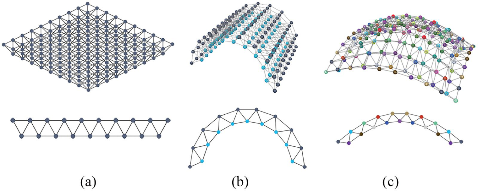
Zero or constant curvature of the design surface allows for uniform joint angles throughout the space-frame layers, while joints in freeform configurations have varying angles: (a) zero curvature, κ = 0; (b) constant curvature, κ = 1/r; and (c) varying curvature, κ = f(x).

Angle calculation

The first step towards the comparison of a structure’s joints according to their geometry is the calculation of the angles between their members. Existing methods for the calculation of joint angles are restricted to two-dimensional grid structures.¹⁹ Personal communication of the authors with fabricators of space-frame structures provided insight into a different approach, used in practice.⁷ In this method, an external reference point is defined, from which the polar angles of the joints are calculated. Nevertheless, this method is highly dependent on the selection of the external reference point, as joints of identical angles will yield different polar coordinates, if their position relative to the reference point is different. It becomes evident, therefore, that there is a need to establish a generalized method for the evaluation of joints according to their local geometrical characteristics, irrespective of their relationship to any external reference. This renders the methods previously presented impractical.

Joint tolerance

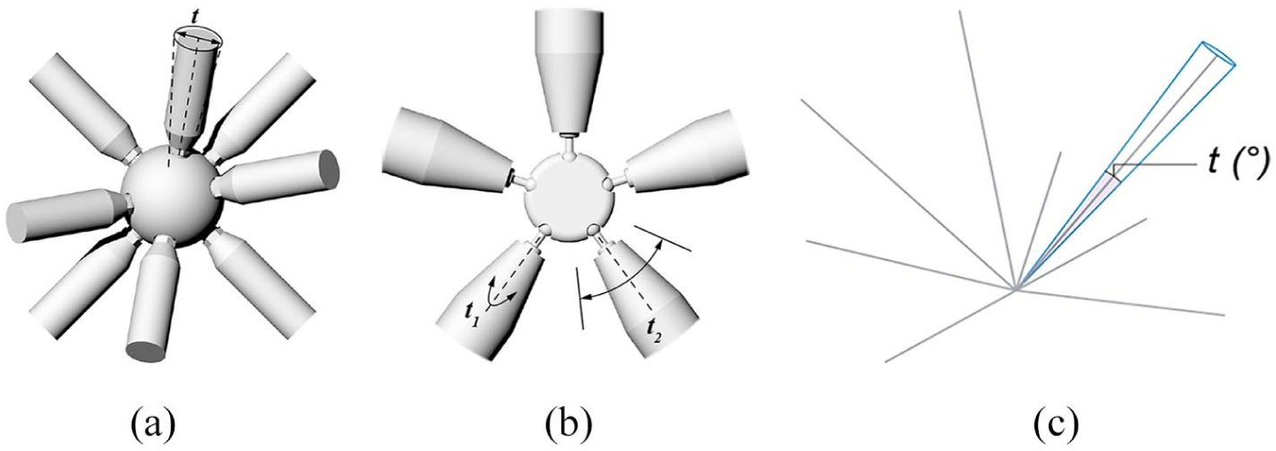
The design and manufacturing of a joint has a significant impact on a structure’s ability to accommodate geometrical variation. Every joint has an embedded capacity to accommodate tolerance, t, in the angles of its members, which is dependent on three factors: (a) the precision of the manufacturing equipment, (b) the joint design and (c) the tolerance induced during construction. The continuous advances in the efficiency of manufacturing equipment has significantly reduced the tolerance linked to manufacturing.²⁰ The joint shown in Figure 2(a), for example, allows for geometrical variation of only 0.01°, as defined by the tolerance of the robotic equipment drilling the holes into the metal sphere.^7,21,22 The design of a joint, however, can accommodate significantly higher levels of tolerance. The joint design presented in Figure 2(b) allows members to move on a plane with a tolerance of up to 180^°.^23–25 Even in joints of Figure 2(a), where the design does not permit any variation, a small number of tolerance is still allowed in practice, to respond to uncertainties that may arise during the construction process.^8,26–28 The precise value of this tolerance is project-specific and depends on the member’s properties, as bending the member to fit in position induces additional stresses to it. There is, hence, a final tolerance that a joint can accommodate, which is a combination of its fabrication, its design and assembly process. Even a few degrees of such tolerance can generate considerable geometrical variation in the final structure.²⁹ For the scope of this study, it is considered to be radially distributed around its members’ centroid axis and the magnitude is defined by the requirements of each project (Figure 2(c)).

Figure 2.

(a) A spherical ball joint with a minimal tolerance of 0.01°.⁷ (b) This joint design allows members’ different tolerances, depending on the plane of movement. The design represents the joint design of ‘hubs’.²⁴ (c) The tolerance, t, of a joint, as considered in this study.

Fabrication process

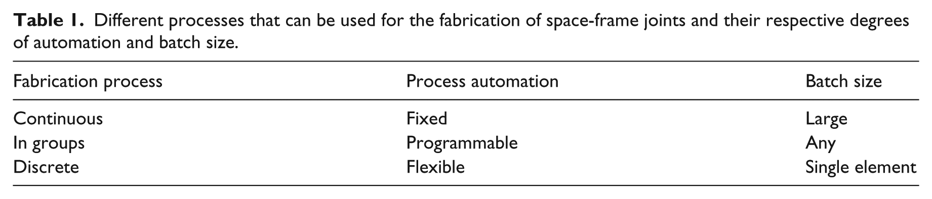
For the scope of this study, fabrication processes are classified according to the size of the batches in which joints are manufactured and the process automation. Batch sizes can vary from large quantities (continuous process) used in mass production to a few (semi-continuous process) or a single joint (discrete process).⁶ Regarding automation, a fabrication process has either hard/fixed-position automation, when the equipment is configured once, a programmable automation, when configured a few times during production, or flexible/soft automation, when configuration takes place at frequent intervals.⁶ A classification of fabrication processes according to these criteria provides an insight into the level of customization allowed for, in combination with the production rate of a specific process, as described in Table 1.

Continuous fabrication

Continuous fabrication produces large quantities of standardized elements in an automated process and in a short period of time.⁶ It includes methods such as metal rolling or casting with permanent moulds. Due to the high cost and time associated with the setting up of the equipment, continuous processes are not considered customizable,⁶ allowing only for an initial set up of the joint configuration before the production begins. This favours standardized products and high production rates. The resulting tolerance that joints produced with continuous processes can accommodate is specific to each joint’s design and is commonly restricted to a small value (Table 1).³⁰

Table 1.

Different processes that can be used for the fabrication of space-frame joints and their respective degrees of automation and batch size.

Fabrication process	Process automation	Batch size
Continuous	Fixed	Large
In groups	Programmable	Any
Discrete	Flexible	Single element

Fabrication in groups

Rapid tooling refers to the use of rapid prototyping for the production of the equipment, rather than the end product. Both subtractive and additive rapid prototyping can be applied to the production of moulds in which the joint is cast.^31,32 The life cycle of each mould is shorter than that of large-scale equipment used in continuous fabrication processes. It is therefore used for a number of casts, until it deteriorates and is then ideally recycled.³³ The production of smaller groups of identical elements has a significant benefit on the overall process. First of all, it introduces a programmable automation,⁶ since the time-expensive method of additive manufacturing is set up and applied only for the printing of the moulds at specific intervals. Moreover, given that casting is an established fabrication process, no certification of the final products’ properties is required. Finally, a level of customization is introduced, since different groups of joints can accommodate any difference between their members geometry.

Discrete fabrication

In discrete fabrication processes, joints are produced individually, forming single-element batches. They are therefore fully flexible in terms of variance, allowing for the production of bespoke elements and ensuring a high degree of customization. The methods range from traditional metal casting with expendable moulds and metal forging, to contemporary methods of rapid prototyping. In particular, rapid prototyping can be both subtractive (computerized numerical control (CNC)) and additive (3D printing)⁶ and allows for computer-based information to be translated to equipment-readable format. It therefore reduces the production time from design to manufacturing significantly and allows for high accuracy and complexity to be incorporated into the joint design. This freedom enables the consideration of multiple optimization criteria within the design of individual joints, further improving their performance.²³ Nevertheless, continuously optimizing the design of a joint and increasing the complexity of its design also increases the time and computational resources required for its production. In effect, this process can become inefficient when the production of a large number of joints is required. Furthermore, this process is subjected to significant size limitations of the final product due to constraints of the 3D printing hardware. More importantly, the end products require bespoke certification of their material properties, as their long-term performance in terms of fatigue and wear is suspect. The overall production time and cost is therefore further increased. However, despite these challenges, research on the practical application of rapid prototyping in the construction industry is continuously evolving to address these challenges.³⁴

Taking into account the fabrication methods described above, it is evident that the quantity of joints and the level of customization required is a key driver in identifying the optimum fabrication process for a given design. Since these factors are project-specific, a single definitive evaluation is not possible. Nevertheless, the flexibility of the fabrication in groups process, which allows for some combination of standardization and customization, makes it worthy of further investigation. Standardized and repeating joints reduce the fabrication time and facilitate erection time, hence providing a safer working environment and reducing cost.³⁵ At the same time, the degree of customization incorporated between different joint groups allows the final space-frame structure to approximate complex freeform surfaces. Achieving complete repeatability of components in complex structures is not feasible.³⁶ Nevertheless, maintaining standardization above a specific threshold allows cost savings from batch production to compensate for the increased cost of bespoke elements.

Methodology

Problem specification

The methodology developed in this article optimizes the geometry of doubly curved space-frame structures to reduce the number of different joint groups required for their construction. It consists of four steps that are cyclically repeated until convergence is reached:

The angles of a space-frame’s joints are calculated in relation to a local coordinate system (angle calculation);

The joints are clustered into the minimum number of groups that satisfy a given tolerance, t (clustering analysis);

The variables of the optimization process are defined according to the curvature of the design surface (control surface);

The space-frame depth is optimized to reduce the number of joint clusters (geometry optimization).

This workflow has been implemented in Grasshopper, the parametric modelling environment of Rhino 3D,³⁷ with custom components coded in C#. The popularity of this software in the industry, and the intuitive user interface, enhances the applicability of this tool in practice.

An architectural design surface, S, is given as a user input, with an initial discretization mesh, representing the top layer of the space-frame structure (Figure 3(a)). There are no restrictions regarding the topology or uniformity of the discretization mesh. Methods for generating meshes on freeform surfaces are described in Pottmann et al.¹⁸ and Stouffs and Sriyildiz.³⁸ The space-frame structure is generated from the mesh according to the method described in Koronaki et al.³⁹ The top-layer vertices, V_t, are considered fixed in position, in order to represent the architectural design surface, while the bottom-layer vertices, V_b, are free to move (Figure 3(b)). Restricting their movement to the normal to the design surface reduces the translation variables of each joint to one, thus enhancing the optimization process. The doubly curved surface presented in Figure 3 will be used as an example to present the developed methodology, which is then applied to a more complex case study in the next section.

Figure 3.

(a) The target design surface and the generated space-frame structure. (b) Definition of the optimization constraints. The top-layer vertices, V_t, are considered fixed to approximate the design surface, while the bottom-layer vertices, V_b, are free to move.

Angle calculation

The first step is to establish a method for the evaluation of joints according to their geometrical characteristics, irrespective of their spatial orientation, the curvature of the design surface or their relationship to any external reference. For this step, a local coordinate system is required for each joint along with an order to evaluate the members.

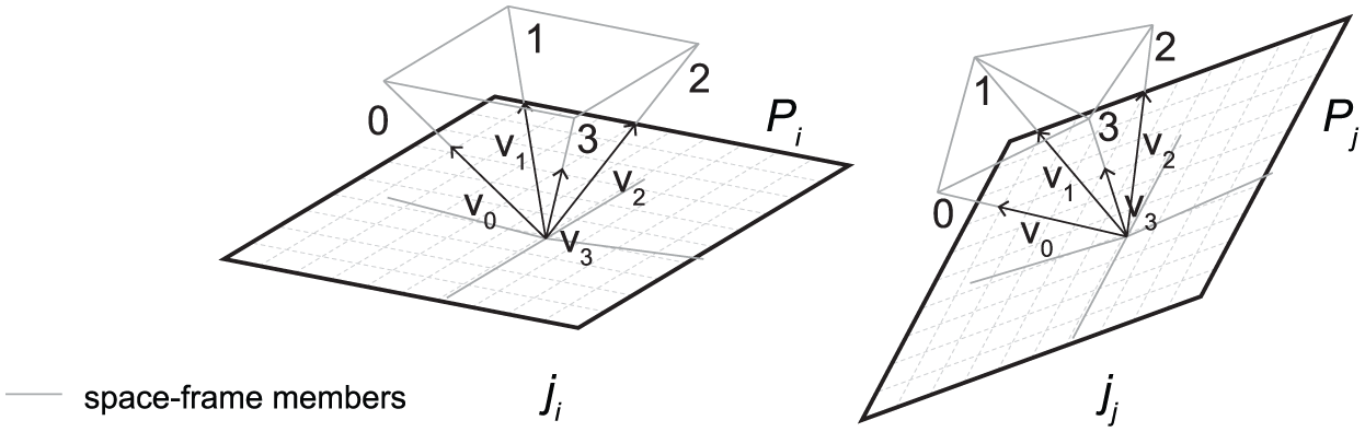
The member vectors, V_i, of each joint, j_i, are unitised and a principal component analysis is carried out, which identifies the best-fit plane, $P_{i}$ , as shown in Figure 4. This plane is specific to the local geometry of each joint, irrespective of its spatial orientation or the topology and curvature of the reference surface it belongs to. Every joint’s best-fit plane serves as a reference for the calculation of the angles between its members.

Figure 4.

A best-fit plane is defined for every joint, serving as a base for the angle calculation.

The vertical angle, $θ$ , between the joint members and the best-fit plane is calculated, and the member forming the largest angle is set as the starting member for the angle calculation, as shown in Figure 5(a). Should multiple members form the same maximum angle, they are all considered as potential starting members and multiple sets of angles are calculated for this joint. The members are then evaluated following a clockwise order when looking down onto the best-fit plane from the end of the starting member (Figure 5(b)). Two values are stored for each member, the angle $ϕ$ with the starting member and the angle $ω$ between their projections onto the best-fit plane when projected along the plane normal (Figure 5(b)). This information is stored in a matrix A[v, k], where v is the maximum valence of any joint in the space-frame and k is the total number of starting members defined for the different joints in the structure (Figure 6). Should a joint have a smaller valence, the remaining rows of the matrix remain empty. Two joints are considered to be identical if they share the same list of angles, in the same order, for at least one of the starting members. In practice, this implies that the two joints could be interchanged in the structure and all members would still ‘fit’. The proposed method forms a robust and computationally efficient method to describe a space-frame’s joints according to their geometry.

Figure 5.

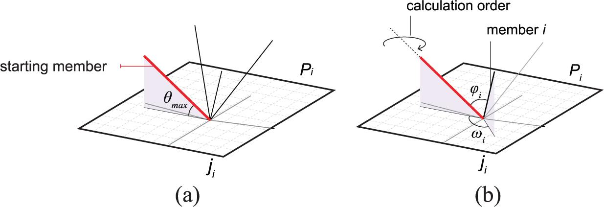
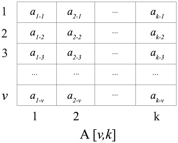
(a) Definition of the starting member and the order for the angle calculation according to the vertical angle, $θ$ , between the members and the best-fit plane. (b) Calculation of angles $ϕ$ and $ω$ between the starting member and member i of the joint.

Figure 6.

Matrix A[v, k], where different angle values of the space-frame structure are stored.

Clustering analysis

This step identifies the number of different joint clusters that are required for the construction of the space-frame structure in compliance with a given tolerance t. Joints of the same cluster will belong to the same batch during the fabrication process, and the similarity measures for the clustering analysis are the angles previously calculated. The maximum angle difference between joints of the same cluster is described as intercluster variance. To ensure compatibility with the prescribed tolerance, t, the maximum intercluster variance should be smaller or equal to the tolerance, t. This forms the driver for the clustering process. Focus is placed on a single-pass clustering algorithm, in which the tolerance, t, is applied as a hard constraint. As opposed to other popular clustering algorithms, such as k-means, in this context, the intercluster variance is an input, driving the clustering process, while the number of clusters, required to achieve it, is the output. This allows for a complete control over the intercluster variance.

The angle difference is calculated for all k(k – 1)/2 possible combinations of joints. Two joints, $j_{i}$ and $j_{j},$ belong to the same joint group if the angle difference between all their members is smaller than or equal to the tolerance, t. The output of this clustering process is the number of clusters, c, required to keep all the joints in groups of maximum tolerance, t.

Geometry optimization

The geometry optimization of the space-frame minimizes the number of clusters, c, required for its construction. As previously mentioned, the tolerance, t, of the clusters forms a hard constraint in the clustering process. A penalty function, p(x), is defined to convert the problem into an unconstrained optimization and enhance a smooth, continuous convergence.⁴⁰ When evaluating the angle matrix of each angle type, a penalty is applied to the values exceeding the tolerance limit, t. A pilot study on the form of the penalty function determined that a quadratic loss function gave good convergence, such that p(x) = max(0, x – t)², where x is the angle difference between the members evaluated and t the tolerance allowed for. The tangential configuration of the parabolic formulation guarantees a rapid convergence rate (Figure 7). The output of the clustering process, therefore, includes a total penalty, p, for the structure and the objective function of the optimization is defined as follows

m i n c x \sum_{i = 0}^{n} p_{i} (x),

where p(x) = max(0, x – t)², in which x is the angle difference between the members evaluated; t is the tolerance allowed for; c is the number of clusters, as defined by the clustering analysis; and n is the number of joints in the structure.

Figure 7.

Graphical representation and formulation of the penalty function, p(x). The tangential configuration and the steep curvature ensure a quick convergence rate.

Control surface

During the geometrical optimization process, the top-layer vertices are fixed in position, while the bottom-layer vertices are free to move along the surface normal. Considering every vertex of the bottom layer as a variable allows for an extensive evaluation of the design space. Nevertheless, it could lead to an impractical and computationally expensive optimization process when applied to large-scale structures.

A control surface is therefore generated to reduce the number of variables in the optimization process. It is generated as a parametric NURBS surface representing the bottom layer of the space-frame. Every bottom layer vertex $(V_{i})$ is mapped on the control surface $({V^{'}}_{i})$ . Any change in the geometrical configuration of the control surface can be traced by the updated position of ${V^{'}}_{i}$ and thus reflected back on the geometry of the bottom-layer vertex, $V_{i}$ (Figure 8). This, in effect, alters the structural depth of the space-frame structure and the number of different joint clusters required.

Figure 8.

(a) Gaussian curvature analysis of the design surface and the respective weighting of the bottom-layer vertices. (b) Mapping of the bottom-layer vertices with their respective weights on the control surface. (c) Indicative selection of control points on the control surface in areas that correspond to a high degree of changing curvature of the design surface.

A crucial factor in this method is the definition of the number and position of the control surface’s control points. As previously described, areas of constant or zero curvature permit the use of a single joint type per layer when the depth is constant, whereas areas of changing curvature require multiple joint groups. The position of the NURBS surface’s control points is thus chosen in relation to the curvature change of the design surface. Controlling the structural depth in the areas of changing curvature can significantly affect the overall number of joint clusters required. The bottom-layer vertices are evaluated according to the Gaussian curvature of the design surface, as shown in Figure 8(a). This evaluation is projected on the control surface (Figure 8(b)), and the ones located in the areas of the highest degree of changing curvature are defined as the control points of the control surface (Figure 8(c)). The exact number of selected control points is dependent on the scale of the structure and the degree of accuracy desired by the designer. Control points can also be defined in the areas of the control surface that do not correspond to positions of bottom-layer vertices. In the case of small-scale structures, it might be feasible to allocate every vertex of the bottom layer as a control point for the control surface, leading to a thorough search of the design space and helping to identify the optimum solution.

Structural depth optimization

Once the control points have been defined, the translation depth for the bottom-layer vertices needs to be determined for the optimization process. A large domain for the depth provides sufficient flexibility to the joints, increasing the design space of possible solutions and thus the possibility of finding more efficient configurations. Nevertheless, increasing the depth above a certain threshold can pose the risk of intersecting members, depending on the geometry of the starting space-frame structure. Therefore, the final domain for the depth values should be determined after both these parameters have been considered and weighted, according to the requirements of the specific project.

The computational workflow presented optimizes freeform space-frame structures to reduce the geometrical variability in their joints and decrease the complexity associated with their construction (Figure 9). A case study analysis follows, which is based on the structure of a real-scale building of complex geometry. The goal of this study is to validate the applicability of the proposed workflow on large-scale structures and evaluate the degree to which it can improve the complexity of their construction process.

Figure 9.

Flowchart representing the workflow of the proposed method.

Case study

The proposed methodology was applied and evaluated on a case study based on the geometry of the Heydar Aliyev Center, designed by Zaha Hadid Architects in Baku, Azerbaijan,¹ which was used due to its complex geometry and large scale. It comprises of two buildings, a library auditorium and a museum. Its structure is a space-frame of a complex, freeform geometry that covers an area of approximately 28,000 m².¹ It is formed by a quadrilateral top-layer grid, while the bottom layer is its dual offset. Diagonal members provide inter-layer connection. The focus of this study is the museum structure. Its geometry was digitally recreated, as shown in Figure 10, according to the information provided in Sanchez-Alvarez¹ and Winterstetter and Toth,⁴¹ with a continuous structural depth of 1 m and a grid spacing of approximately 2.3 × 2.3 m². The generated geometry forms a credible approximation of a real-scale, complex structure and was used as a starting space-frame configuration, which was then analysed and optimized.

Figure 10.

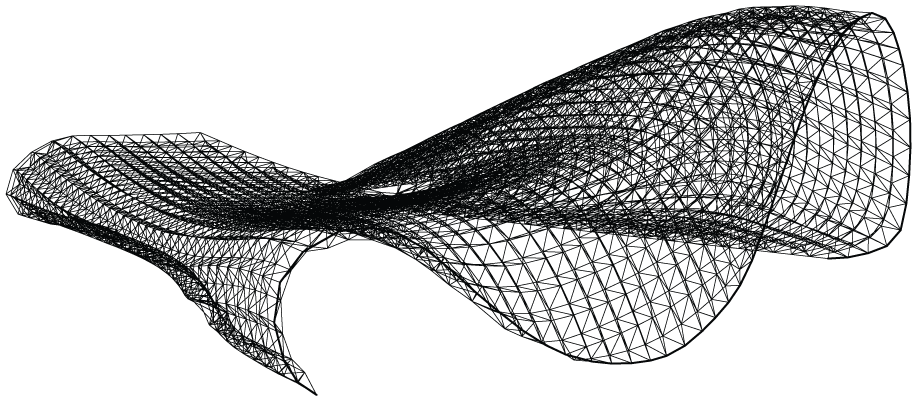
A three-dimensional view of the Heydar Aliyev Museum grid structure.

The generated starting grid of the museum comprises of 3018 joints, 1541 in the top layer and 1477 in the bottom. The number of clusters that these joints can be grouped into is dependent on the prescribed tolerance, t, as demonstrated in Figure 11. The steep gradient of the curve for tolerances t ⩽ 10° outlines the high impact that the tolerance plays in defining the number of different joint groups, especially when its value is low. For tolerances t > 10°, this impact is less pronounced, with the number of different joint groups gradually decreasing, until they reach the value of 1 for tolerances t ⩾ 86°. For this study, a tolerance of t = 3° was considered, which corresponds to 1067 different joint groups. Its low value ensures its high impact on the clustering process, while at the same time renders it realistic, when considered as a factor of the manufacturing process, the joint design and the tolerance induced during the assembly process, as previously described.

Figure 11.

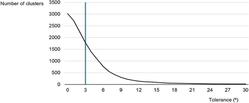
Relationship between the joint tolerance and the number of different joint groups for the museum space-frame structure.

A control surface was generated to define the variables of the optimization process. The bottom-layer vertices were projected on it and evaluated according to the curvature analysis of the museum’s top-layer surface (Figure 12). It should be highlighted at this point that, when the control surface approach is applied on space-frames of double curvature, such as the museum structure, there is a distortion when mapping the vertices from a doubly curved domain onto a flat surface. Nevertheless, these limitations are not significant and are a price worth paying, considering the dimension reduction of the optimization complexity.

Figure 12.

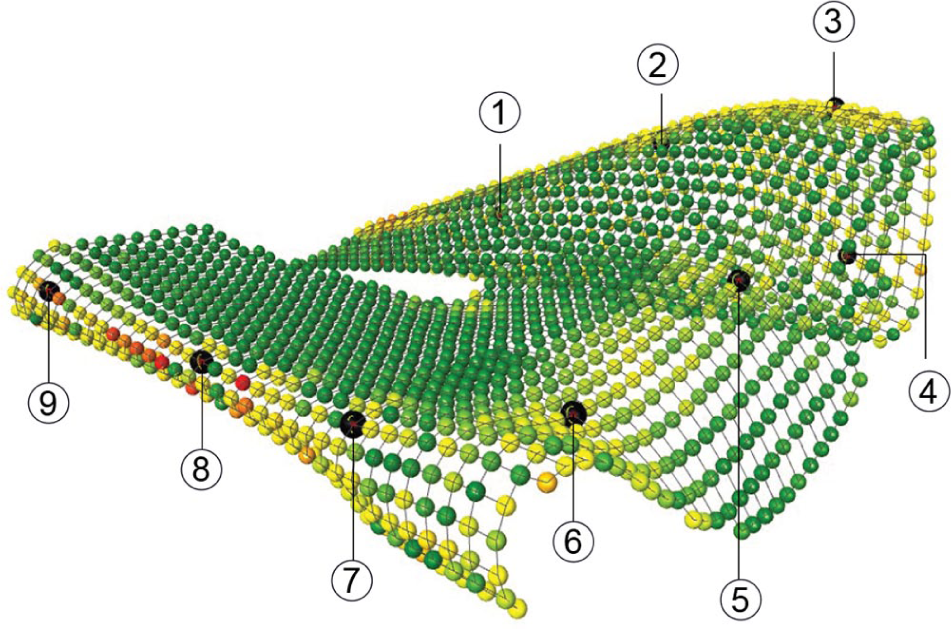
The control points are defined on the structure according to the curvature analysis of the design surface. They are afterwards mapped on the control surface for the optimization process.

Nine vertices of the bottom layer were selected as control points for the control surface, as shown in black colour in Figure 12. Their position in areas of high changes of curvature provides a direct link between the structure’s geometry and the optimization process. The fact that they are distributed across the whole area of the control surface ensures a directed and informed change in the depth of the whole structure. Controlling the position of the 1477 vertices of the bottom layer by only 9 control points renders the optimization highly effective in terms of computational resources required.

An optimization was carried out to minimize the number of different joint groups. The NURBS surface’s control points were defined as variables with a domain of [0.5, 10] m for structural depth. The limits of this domain were defined to avoid any intersection between structural members while ensuring sufficient translation freedom. The workflow previously described provides a framework for the optimization, which can be carried out with different optimization algorithms. Considering the size and variability of the design space, a pilot study was run to compare the efficiencies of a simulated annealing solver and genetic algorithm,^42,43 with the latter achieving improved results for a population size of 200 and a mutation rate of 10%.

Results

The optimization process achieved an overall reduction of 15% in the number of joint clusters from 1067 to 904. An interesting observation is that even though the variables’ domain was [0.5,10] m, the output values of the structural depth remained within the range of 0.5–0.8 m, which are similar to, or slightly smaller than, the values in the starting grid configuration. This highlights the fact that minor changes in the geometry can lead to significant savings in the construction process of a structure.

Even though the optimization process focuses on the geometry of the space-frame structure, changes in its configuration have a direct impact on the structural performance as well. To evaluate the validity of the results, a structural analysis was carried out on the starting space-frame and the optimized structure. Circular solid sections were considered for the space-frame members with a constant cross-section per layer (top-, bottom- and inter-layer connections). The load case applied in the analysis was the structure’s self-weight and a combination of additional dead and live loads of 2.2 kN/m². Both values were factored for the ultimate and service limit state analyses, in compliance with the EN1991 standards. The material applied was steel S355 (Young’s modulus = 2.1 × 10⁷ kN/m², density = 79 kN/m³, modulus of rupture = 3.6 × 10⁵ kN/m²). The mass of the structure was calculated for a maximum utilization of 0.8 and resulted in a structural weight of 240 t for the starting structure and 184 t when optimized. Apart from reducing the number of different joint groups, the optimization process, hence, also led to a significant reduction of 23% in mass. It should be highlighted, of course, that since the optimization was carried out on a geometrical basis and focused on the joint variability, the reduction in the mass should not be considered as an effect that takes place whenever the proposed method is applied. The important observation of the structural analysis conducted is the fact that, the proposed method led to a significant reduction in the construction complexity, without compromising the structural performance.

Conclusion

The proposed workflow provides an effective framework to facilitate the construction process of freeform space-frame structures by reducing the variability in its members. The case study presented highlights the potential of its application on real-scale complex structures, achieving a 15% reduction in the number of joint clusters, with minor changes in the overall geometry and without compromising the structural performance.

A novel method was developed for the calculation of the angles of space-frame joints. The effectiveness of the method lies in the fact that the comparison is solely based on a local coordinate system that is specific to each joint, according to its geometrical characteristics. This fact renders this method applicable to any freeform structure, irrespective of the geometry of the design surface. Once the joint angles have been calculated, a clustering analysis is carried out, using the tolerance, t, of the fabrication process as a hard constraint. Running in a single pass, this process provides accurate and time-efficient clustering. Nevertheless, it is dependent on the input order of the data. Future work of the authors will focus on alternative methods of formulating the algorithm for the grouping of joints, which will combine dynamic clustering with control over the final variance of the clusters. An iterative clustering analysis allows the exploration of a larger extent of the design space and can hence yield improved results in terms of intercluster variance.

The use of a control surface to define the optimization variables forms one of the integral parts of the workflow developed. The essential benefit of this process lies in the fact that it allows a reduced number of parameters, independent of the scale of the structure. It therefore lends itself well to the optimization of complex, large-scale structures, where reducing the construction complexity can lead to significant savings. In the case study presented, for example, using all 1477 vertices of the bottom layer as variables would have resulted in a design space of 3.3 × 10²⁸ solutions. Through the application of the control surface, however, only nine control points were used, leading to a huge reduction in the size of the design space to 1.1 × 10¹⁸ solutions. Overall, designers are given the freedom to select the number of control points according to the degree of detail they desire and the computational resources available. In small-scale problems, defining every vertex as a variable allows for an in-depth exploration of the design space and can yield optimum solutions. Irrespective of their number, however, linking the control points to the curvature change of the design surface improves the response of the optimization process to project-specific requirements and hence enhances its performance. In addition, this forces a smooth transition of structural depth between neighbouring joints, which is aligned with architectural design criteria for visual continuity.

The proposed computational workflow achieves an increasing joint uniformity in 3D space-frames in a practical and efficient manner. Through an automated and computationally efficient workflow, it provides direct insight into the fabrication complexity of a given structure in the early design stages. This process can substantially reduce the complexity of the fabrication and construction of space-frame structures and the associated cost, time and labour. These findings therefore suggest an overall shift of the complexity from the construction to the design process, where it can be dealt with by the application of the advanced computational workflow proposed. This enables designers to propose more complex geometries, making use of new advances in fabrication processes and generating better engineered solutions.

Footnotes

Acknowledgements

The authors would like to express their gratitude to LANIK Engineers and particularly to Goni Josu and Alain Cabanas for their support. Moreover, they would also like to thank Jaime Sanchez-Alvarez and Salome Galjaard for their views and insights into the opportunities and challenges in the construction of space-frame structures in practice.

Declaration of conflicting interests

The author(s) declared no potential conflicts of interest with respect to the research, authorship, and/or publication of this article.

Funding

The author(s) disclosed receipt of the following financial support for the research, authorship, and/or publication of this article: This study was supported by the EPSRC Centre for Decarbonisation of the Built Environment (dCarb; Grant Ref. EP/L016869/1) and the Engineering & Physical Sciences Research Council [Grant Ref: EP/N023269/1].

ORCID iDs

Antiopi Koronaki

Paul Shepherd

References

Sanchez-Alvarez

. Practical aspects determining the modelling of the space structure for the free-form envelope enclosing Baku’s Heydar Aliyev Cultural Centre. In: Proceedings of the 50th international association for shell and spatial structures evolution and trends in design, analysis and construction of shell and spatial structures, Valencia, 28 September–2 October 2010, pp. 1263–1274. Valencia: Universidad Politecnica de Valencia.

Tsigkari

Olsson

Aish

, et al. The computational challenges of a mega space frame shaping the envelope of New Mexico City airport. In: ACADIA 2017: Disciplines & disruption: proceedings of the 37th annual conference of the association for computer aided design in architecture (ACADIA), Cambridge, MA, 2–4 November 2017, pp. 620–629. Cambridge: Acadia Publishing Company.

Klimke

Sanchez-alvarez

Vasiliu

, et al. The envelopes of the arts centre in Singapore, 2002, https://www.researchgate.net/publication/233582234

Søndergaard

Amir

Knauss

. Topology optimization and digital assembly of advanced space-frame structures. In: Adaptive architecture: proceedings of the 33rd annual conference of the association for computer aided design in architecture (ACADIA 13), Cambridge, 24–26 October 2013, pp. 367–378. Toronto: Riverside Architectural Press.

Fischer

. Generation of apparently irregular truss structures. In: Proceedings of the 11th international CAAD futures conference, Vienna, 20–22 June 2005, pp. 229–238. Dordrecht: Springer.

Kalpakjian

Schmid

Sekar

Manufacturing engineering and technology. 7th ed. Cambridge: Pearson, 2007.

LANIK Engineers. Hacemos su proyecto realidad, http://www.lanik.com/ (accessed 8 November 2019)

Lan

TT.

Space frame structures. In: Wai-Fah

(ed.) Structural engineering handbook. Boca Raton, FL: LLC, CRC Press, 2005, pp. 1–50.

Koronaki

Shepherd

Evernden

Geometry optimization of space frame structures for joint modularity. In: Adriaenssens

Mueller

(eds) IASS annual symposium: creativity in structural design, Boston, MA, 16–20 July 2018.

10.

Dritsas

Design-built rationalization strategies and applications. Int J Archit Comput 2012; 10(4): 575–593.

11.

Ranalli

Flager

Fischer

A Ground Structure Method to Minimize the Total Installed Cost of Steel Frame Structures. Int J Civ Environ Eng 2017; 12(2): 160–168.

12.

Havelia

A ground structure method to optimize topology and sizing of steel frame structures to minimize material, fabrication and erection cos. Stanford, CA: Stanford University, 2016.

13.

Paulson

Designing to reduce construction cost. J Constr Div 1976; 102(4): 587–592.

14.

Dritsas

Chen

Sass

. Small 3D printers/large scale artifacts: computation for automated spatial lattice design-to-fabrication with low cost linear elements and 3D-printed nodes. In: Proceedings of the 22nd international conference on computer-aided architectural design research in Asia: protocols, flows and glitches, Suzhou, China, 5–8 April 2017, pp. 821–830. Suzhou, China: Xi’an Jiaotong-Liverpool University.

15.

Chun

Lee

Park

. Topo-joint: topology optimization framework for 3D-printed building joints. In: Proceedings of the 23rd international conference of the association for computer-aided architectural design research in Asia (CAADRIA), Beijing, China, 17–19 May 2018, pp. 205–214. Hong Kong: Association for the Computer-Aided Design Research in Asia (CAADRIA).

16.

Sousa

Varela

Carvalho

. Mass-customization of joints for non-standard structures through additive manufacturing: the Trefoil and the TriArch projects. In: Ecaade36: applications in construction & optimization, Lodz, 19–21 September 2018, pp. 197–204. Lodz: Lodz University of Technology.

17.

Gheorghiu

Dragomir

Manoil

Geometry of structural forms. London: Applied Science Publishers, 1978.

18.

Pottmann

Asperl

Hofer

, et al. Architectural geometry (ed. Bentley

). Exton, PA: Bentley Institute Press, 2007.

19.

Stephan

Sánchez-Alvarez

Knebel

Stabwerke auf Freiformflächen. Stahlbau 2004; 73(8): 562–572.

20.

Wang

Liu

Sparks

, et al. Industrial robot trajectory accuracy evaluation maps for hybrid manufacturing process based on joint angle error analysis. Adv Robot Autom 2018; 7(1): 183.

21.

Octatube. Realizing challenging architecture, https://www.octatube.nl/ (accessed 8 November 2019).

22.

MERO. https://www.mero.de/ (accessed 8 November 2019).

23.

Galjaard

Hofman

Perry

, et al. Optimizing structural building elements in metal by using additive manufacturing. In: Proceedings of the international association for shell and spatial structures (IASS) symposium, Amsterdam, 17–20 August 2015.

24.

hubs. geodesic domes made simple, https://buildwithhubs.co.uk/ (accessed 8 November 2019).

25.

Rochas

Patent 8,820,025 B1, USA, 2014, https://patentimages.storage.googleapis.com/48/20/f6/bf9308c6670137/US8820025.pdf

26.

Ariza

Mirjan

Gandia

, et al. In place detailing. ACADIA, 2018, pp. 312–321, http://papers.cumincad.org/data/works/att/acadia18_312.pdf

27.

Wallick

. Digital and manual joints. In: ACADIA 08: silicon + skin: biological processes and computation: proceedings of the 28th annual conference of the association for computer aided design in architecture, 2008. pp. 370–375, http://papers.cumincad.org/data/works/att/acadia08_370.content.pdf

28.

Méndez Echenagucia

Pigram

Liew

, et al. A cable-net and fabric formwork system for the construction of concrete shells: design, fabrication and construction of a full scale prototype. Structures 2019; 18: 72–82.

29.

Motro

Nodes and structures – a tribute to Stephane Du Chateau. In: International association for shell and spatial structures: beyond the limits of man, Wroclaw, 2013, pp. 1–5, https://hal.archives-ouvertes.fr/hal-00867855

30.

Gonzalez Bravo

. Aplicaciones industriales para la construcción de estructuras laminares metálicas. PHD Thesis, Escuela Tecnica Superior de Arquitectura de Madrid, Madrid, 2015.

31.

Aghaei Meibodi

Giesecke

Dillenburger

. Digital metal: additive manufacturing for casting metal parts in architecture, https://www.research-collection.ethz.ch:443/handle/20.500.11850/322205 (2018, accessed 8 November 2019).

32.

Aghaei Meibodi

Giesecke

Dillenburger

. 3D printing sand molds for casting bespoke metal connections. Intelligent & informed: 24th annual conference of the association for computer-aided architectural design research in Asia (CAADRIA), Wellington, New Zealand, 15–18 April 2019, pp. 133–142. Hong Kong: Association for the Computer-Aided Design Research in Asia (CAADRIA).

33.

Niehe

Sand printing makes complex casted structural parts affordable. Amsterdam, Europe Press Office, 2017.

34.

Wang

A critical review of the use of 3-D printing in the construction industry. Autom Constr 2016; 68: 21–31.

35.

BCSA/SCI Connections Group. Joints in steel construction: simple joints to Eurocode 3. London: The Steel Construction Institute, The British Constructional Steelwork Association Limited; 2011.

36.

Lindsey

Digital Gehry: material resistance, digital construction. Basel: Birkhauser, 2001.

37.

Rhino 6 for Windows and Mac, https://www.rhino3d.com/ (accessed 8 November 2019).

38.

Stouffs

Sriyildiz

(eds). eCAADe 2013: computation and performance, vol. 1, 2013, https://publons.com/journal/135125/ecaade-2013-computation-and-performance-vol-1

39.

Koronaki

Shepherd

Evernden

. Layout optimization of space frame structures. In: Proceedings of the IASS Annual Symposium, Hamburg, 25–28 September 2017.

40.

Yeniay

. Penalty function methods for constrained optimization with genetic algorithms. Math Comput Appl 2005; 10(1): 45–56.

41.

Winterstetter

Toth

Engineering complex geometries – the Heydar Aliyev Centre in Baku. Steel Constr Des Res 2015; 8(1): 65–71.

42.

Rutten

Evolutionary principles applied to problem solving, 2013, pp. 1–26, http://www.grasshopper3d.com/profiles/blogs/evolutionary-principles

43.

Rutten

. Navigating multi-dimensional landscapes in foggy weather as an analogy for generic problem solving. In: Proceedings of the 16th international conference on geometry and graphics, Innsbruck, 4–8 August 2014, p. 14. Innsbruck: ISGG.