Testing and correcting for spatial unit roots in regression analysis

Abstract

Spatial unit roots can lead to spurious regression results. We present an overview of the methods developed in Müller and Watson (2024, Econometrica 92: 1661-1695) to test and correct for spatial unit roots and introduce a suite of commands (spur) implementing these techniques. Our commands exactly replicate results in Müller and Watson (2024) using the same data as Chetty et al. (2014, Quarterly Journal of Economics 129: 1553-1623). As a guide for applied researchers, we provide a practical algorithm for regression analysis using these methods and a simulated illustration in Stata.

Keywords

st0802 spur spurtest spurtransform spurhalflife spurious spatial regression spatial unit roots

1 Introduction: Spatial unit roots

Spatial data present challenges for statistical analysis: observations that are close to each other geographically tend to be correlated, violating the assumption of independent and identically distributed (i.i.d.) errors. In such settings, heteroskedasticity- and autocorrelation-consistent (HAC) corrections or clustered standard errors at broader geographic levels (like states) are often used.

However, these correction methods fail when spatial dependence is too strong (“spatial unit roots”). Even with clustering or HAC corrections, spuriously significant regression coefficients can arise. Müller and Watson (2024) developed new statistical tests to detect such strong dependence and procedures to correct for it, extending techniques from time-series analysis. We present a Stata implementation of their original MATLAB code, along with practical guidelines for applied researchers.

In the time-series context, weak serial correlation in the regressors and regression errors [the I(0) case] can be dealt with by HAC corrections. However, when the serial correlation is strong [the I(1) case], inference fails and ordinary least-squares (OLS) produces “spurious regressions” (Granger and Newbold 1974). Furthermore, test statistics behave in nonstandard ways (Phillips 1986).

The spatial context is similar (Fingleton 1999), but as Müller and Watson (2022) discuss, there are also important differences: First, time-series operate in a one-dimensional space, whereas in the spatial context, we are dealing with two (or three) dimensions. Second, in the time-series context, observations are usually equally spaced (…, t — 1, t, t + 1,…), whereas in the spatial context, the location of observations on a map can be substantially different from a uniform distribution on a grid. Third, while there is a directionality in the time-series context (…, t — 1, t, t + 1,…), in the spatial context, going east is as natural as going west or north or south. Müller and Watson (2022) propose a method for constructing confidence intervals that accounts for many forms of spatial correlation. It uses a projection-type variance estimator, where the projection weights are spatial correlation principal components (SCPC) from a given “worst case” benchmark correlation matrix.

Müller and Watson (2022) require stationarity of both regressors and dependent variables for the large-sample validity of their SCPC method. In Müller and Watson (2023), they present a robust version that can deal with some nonstationarities relevant to applied research. The methods developed in these two articles have been implemented in Stata by the authors in their scpc package,¹ which provides a postestimation command to correct regression inference for weak spatial dependence. However, as Müller and Watson (2024) show, these and other spatial HAC methods cannot deal with the case of strong spatial autocorrelation in the outcome of interest. Müller and Watson (2024) introduce diagnostic tests for such spatial unit roots and show how transformations of the dependent and independent variables eliminate spurious regression results in the presence of strong spatial dependence.

In this article, we provide a community-contributed version of the programs developed by Müller and Watson (2024) to test for and correct for spatial unit roots. These methods can be used in conjunction with the scpc package to correct regression inference for remaining weak spatial dependence after spatial unit roots have been corrected, but our package does not depend on scpc and can be used independently. We show that our routines replicate the results in Müller and Watson (2024) using data from Chetty et al. (2014).

We also provide practical guidelines for applied researchers dealing with potential spatial unit roots in regression analysis: how to test for nonstationarity or the presence of spatial unit roots and what to do in case nonstationarity is detected or when the presence of spatial unit roots cannot be rejected. To illustrate this algorithm and the use of our community-contributed commands, we present a simulated example and a Monte Carlo simulation.

The rest of the article proceeds as follows: Section 2 summarizes and illustrates the tests developed by Müller and Watson (2024) to diagnose spatial unit roots, as well as our Stata implementation of their MATLAB code in the commands spurtest and spurhalflife. Section 3 explains the spatial differencing techniques they propose to eliminate unit roots and presents how they can be applied using the command spurtransform. Appendix A demonstrates the functionality of our implementation by replicating results from Müller and Watson (2024). Section 4 presents a brief guide to using these methods in common settings in applied research, illustrated by an example application. Section 5 concludes. A supplemental online appendix contains color versions of figures 1, 2, 3, 4, 6, and 7.

Figure 1.

Spurious correlations with unit roots

Figure 2.

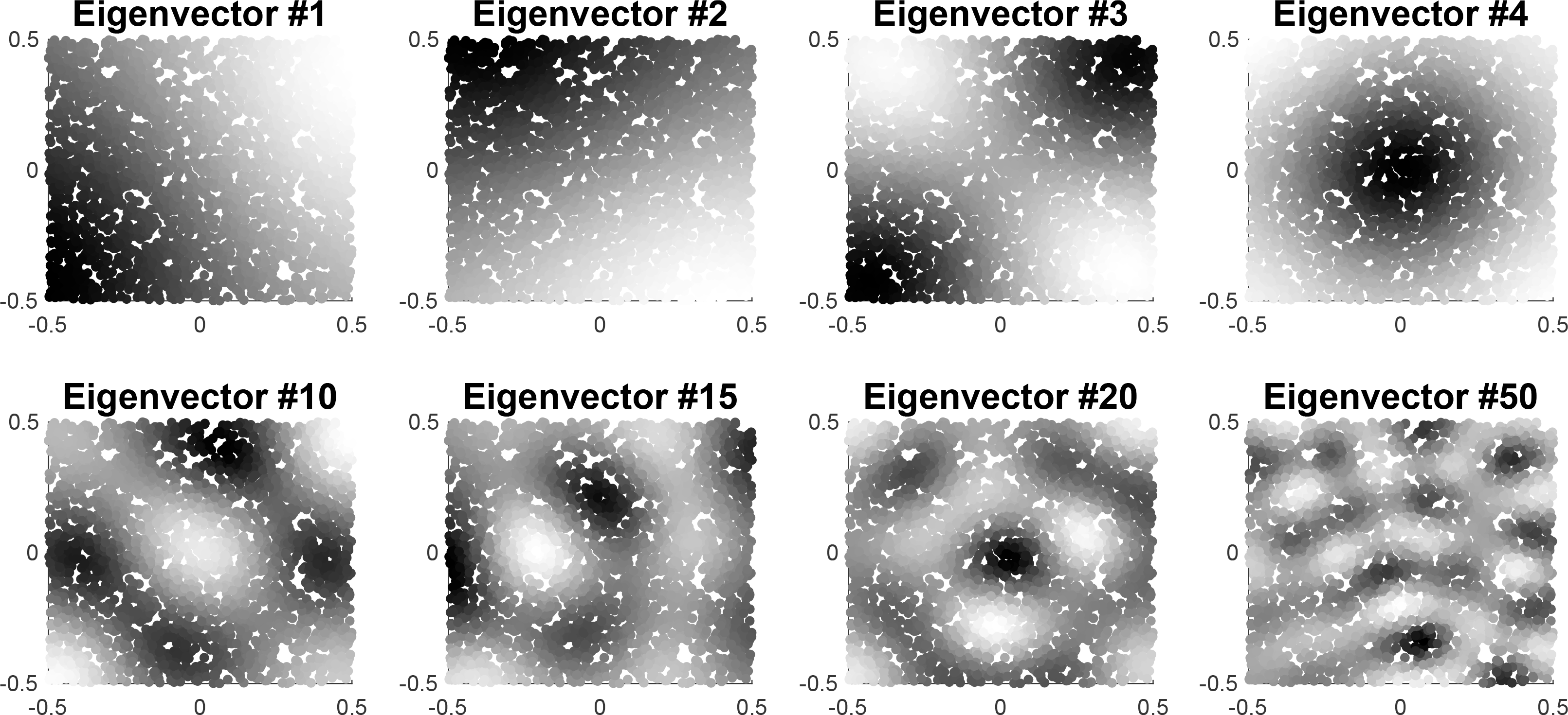
Illustration of the weights

Figure 3.

Simulated data and weighted averages

Figure 4.

Differencing transformations

2 Testing for spatial unit roots

This section discusses the approaches to inference about the degree of spatial dependence developed by Müller and Watson (2024). They motivate their analysis of spatial unit roots by starting from the time-series analogue: in time series, the canonical I(1) process is a Wiener process (also called Brownian motion). Its extension to the (two-dimensional) spatial case is via a so-called Lévy-Brownian motion (LBM). Figure 1 illustrates the similarity between spurious regressions in the time-series context and spatial context: Panel (a) shows realizations of two independent Gaussian random walks, and (b) shows independent simulated spatial unit-root processes over n = 722 US commuting zones. In each case, we report the R² and t statistics from the linear regression (with HAC correction) of the first on the second process, which show spuriously significant correlation in both cases. Panel (c) shows two variables from Chetty et al. (2014): their outcome variable (mobility index) and one regressor (teen labor force participation). These resemble the unit-root processes in panel (b). This highlights the potential relevance of strong spatial autocorrelation, which needs to be detected and addressed in empirical work.

Specifically, Müller and Watson (2024) develop four diagnostic tests, examining the following null hypotheses, respectively:

H₀: Scalar variable y is I(1).

H₀: Scalar variable y is I(0).

H₀: Linear regression residuals u are I(1).

H₀: Linear regression residuals u are I(0).

They also developed a method to construct confidence intervals for the spatial halflife of a scalar variable. All of these tests exploit the different variance-covariance structures implied by the canonical spatial I(1) and local-to-unity (LTU) models (Müller and Watson 2024).

The canonical spatial I(1) model is LBM, a spatial generalization of the Wiener process (Brownian motion) common in time-series analysis. This can be thought of as a continuous-time analogue of a random walk. Conversely, LTU models describe stationary processes with weak mean reversion governed by a parameter c > 0. They are a generalization of the pure unit-root model, in which the autoregressive root approaches unity as the sample size increases at a rate determined by c. This allows them to behave similarly to I(1) processes for small c and similarly to weakly dependent I(0) processes for large c. Thus, they span a continuum of dependence between the dichotomous I(0) and I(1) cases. Their canonical form is the Ornstein-Uhlenbeck process, which can be thought of as a continuous-time analogue of a first-order autoregressive process in the time-series context. The variance-covariance structure of these two canonical models in the spatial case is given by

Canonical I (1) model : y_{l} = L (s_{l}), E {L (s) L (r)} = \frac{1}{2} (| s | + | r | - | s - r |)

Canonical LTU model : y_{l} = J_{c} (s_{l}), E {J_{c} (s) J_{c} (r)} = \exp (- c | s - r |) / (2 c)

where l indexes locations, s,r denote locations in space,

| x | = \sqrt{x^{'} x}

L (\cdot)

is LBM, and

J_{c} (\cdot)

is the spatial generalization of the Ornstein-Uhlenbeck process with mean-reversion parameter c > 0. These canonical processes provide asymptotic approximations for more general models² (see theorem 2 in Müller and Watson [2024]), and their properties can thus be used to discriminate between I(1) and I(0) processes.

2.1 Low-frequency weighted averages

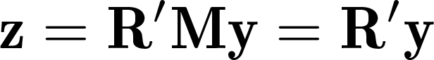
The fundamental idea is to compare the performance of these two models in rationalizing the data. Rather than performing tests on the raw data, Müller and Watson (2024) build on Müller and Watson (2008) and compute the test statistics from a fixed number q of weighted averages of the data. Specifically, given a data vector $y = (y_{1}, \dots, y_{n})^{'}$ . define Σ_L as the n × n covariance matrix of y implied by the canonical I(1) model [LBM L(·)]. In other words, Σ_L is the theoretical covariance matrix of the data under the I(1) model. From this, derive $R$ as the n × q matrix whose columns are the eigenvectors of ΜΣ_LΜ corresponding to the q largest eigenvalues, where $M = I_{n} - 1 (1^{'} 1)^{- 1} 1^{'}$ is the demeaning matrix, and scaled such that $n^{- 1} R^{'} R = I_{q}$ . Then the weighted averages are computed as

z = R^{'} M y = R^{'} y

The

j

(j = 1, \dots, q)

weighted average is the linear combination of the data with the

j

th-largest population variance under the canonical I(1) model; that is, the scalar z_j is the

j

th-largest principal component of

M y

based on the assumed covariance matrix ME _L M. As illustrated below and discussed in detail in Müller and Watson (2019) for the time-series case, this choice of weights extracts and summarizes low-frequency variation in the data.

Basing the tests on these weighted averages is useful in two broad ways: First, summarizing the data in a fixed number of averages yields an asymptotically multivariate (q-dimensional) normal distribution (following from a central limit theorem), which enables the use of standard inference methods. The covariance matrix of this limiting distribution is simply

Var (z) = R^{'} Σ R \equiv Ω

where

Σ

is the covariance matrix induced by the data-generating process. For the purposes of this article,

Σ

will be the covariance matrix implied by one of the two canonical models discussed above, which we denote by

Σ_{L}

for the I(1) model and

Σ (c)

for the LTU model with decay parameter c. They imply different covariance structures Var(z), henceforth denoted as Ω_L and Ω(c). This is exploited to discriminate between broad models of persistence, which reduces to a standard problem of inference about the covariance matrix under normality.³ Second, choosing the weights to extract only low-frequency variation makes the resulting tests robust to misspecification of the high- frequency variation: the accuracy of the approximations derived from the canonical models in finite samples now does not depend (much) on the ability of those models to match the high-frequency behavior of the data-generating process. See Müller and Watson (2019) for a more extensive discussion.

Choice of q. An obvious practical question is how to choose the number of weighted averages q. This requires a tradeoff: a large q increases the amount of data used in the tests, increasing power, but also makes the tests more sensitive to high-frequency noise in the data. Müller and Watson (2024) argue that a q between 10 and 20 captures most of the relevant low-frequency variation and use q = 15 in their applications. Our numerical simulations show that the q = 10 (q = 15) [q = 20] largest eigenvectors capture about 85% (87%) [90%] of the variation in simulated LBM processes, respectively, while q = 30 (q = 50) increases this share only slightly to 92% (94%). In our community-contributed package, all test commands include the option q(). We set q(15) as the default and also recommend that users test the robustness of their results with different choices of q.

Illustration of weighted averages. We illustrate the construction of the weighted averages in a simple example. We randomly draw n = 3000 locations from a uniform distribution on the unit square, with coordinates $s_{i}, l = 1, \dots, n$ . The covariance matrix induced by LBM for these locations is then given by Σ _L , where the $(l, ℓ)$ th element is 1/2 $(| s_{l} | + | s_{ℓ} | - | s_{l} - s_{ℓ} |)$ . From there, it is straightforward to compute the eigenvectors of ΜΣ_LΜ. The subplots of figure 2 show the eigenvectors corresponding to the 1st, 2nd, 3rd, 4th, 10th, 15th, 20th, and 50th highest eigenvalues, respectively, where the color of location l on the map indicates the value of the $l$ th element of the respective eigenvector.

The “frequency” of the variation clearly increases with the order of the eigenvectors. To see how z extracts low-frequency variation from y, notice that $z = R^{'} y = n (R^{'} {R)}^{- 1} R^{'} y$ because $n^{- 1} R^{'} R = I_{q}$ by construction. Therefore, z can also be understood as coefficients (loadings) from projections of y on the q-largest eigenvectors of ΜΣ_LΜ. Inspecting the behavior of these eigenvectors in figure 2 clarifies how this captures low-frequency variation.

This is further illustrated by the subplots of figure 3: The first two subplots show simulated data for an LBM process, y_LBM ∼ N(0, Σ _L ), and an LTU process with much lower persistence, y_LTU ∼ N{0, Σ(10)}, respectively. The difference in low-frequency variation is clearly visible. The third subplot illustrates how the weighted averages discussed above can be used for inference about spatial persistence. The black lines show the absolute values of the elements of $z_{LBM} = R^{'} y_{LBM}$ and $z_{LTU} = R^{'} y_{LTU}$ , respectively, where $R$ collects the eigenvectors of ΜΣ_LΜ corresponding to the q = 15-largest eigenvalues (so that $j = 1$ is the largest eigenvector, $j = 2$ the second largest, etc.). The difference in behavior is stark: the LBM process loads heavily on the first few eigenvectors (low frequencies) and then quickly decays, while the LTU process loads evenly across the spectrum. This empirical behavior can be compared with the expected behavior of z under the two models, given by z_LBM ∼ N(0, Ω_LBM) and z_LTU ∼ N(0, Ω_LTU), respectively, where $Ω_{LBM} = R^{'} Σ_{L} R$ and $Ω_{LTU} = R^{'} Σ (10) R$ . This implies that $E (z_{j}^{2}) = Ω_{j, j}$ for the respective model, shown by the gray lines. By construction, Ω_LBM describes the behavior of z_LBM much better than that of z_LTU, and vice versa. The next sections formalize such comparisons to distinguish between I(1) and I(0) processes.

2.2 Generic testing procedure

Given the weighted averages z, whose limiting distribution is multivariate normal, inference boils down to testing hypotheses about its covariance matrix Ω. In all tests, the hypotheses are of the form

H_{0} : Ω = Ω_{0} versus H_{a} : Ω = Ω_{α}

Müller and Watson (2024) suggest using the likelihood-ratio test statistic of

z / \sqrt{z^{'} z}

\frac{L (Ω_{a} | z)}{L (Ω_{0} | z)} \propto \frac{z^{'} Ω_{0}^{- 1} z}{z^{'} Ω_{a}^{- 1} z} \equiv Λ

with critical value (CV), which solves

Pr (Λ > CV | H_{0}) = α

By the Neyman-Pearson lemma, this is the most powerful level α scale-invariant test. In practice, the CV is computed by

drawing N_rep random q x 1 vectors $\hat{z}$ from the distribution N(0, Ω₀),

computing the test statistic $\hat{Λ} = \hat{z}^{'} Ω_{0}^{- 1} \hat{z} / \hat{z}^{'} Ω_{a}^{- 1} \hat{z}$ for each draw, and

setting CV as the empirical 1 — α quantile of the resulting distribution of $\hat{Λ}$ .

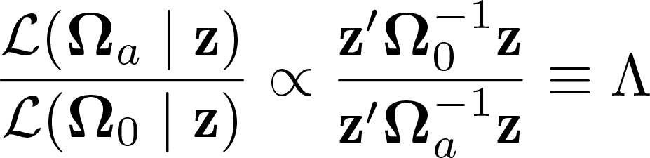
The test then rejects H₀ if Λ > CV.⁴ All test commands in our package include the option nrep(), which sets the sample size N_rep for the Monte Carlo simulation. The default is nrep(100000).

2.3 I(1) test

The I(1) test examines the presence of a unit root in a scalar variable y, that is, the I(1) model versus the LTU model. The hypotheses are therefore

H_{0} : Ω = Ω_{L} = R^{'} Σ_{L} R versus H_{a} : Ω = Ω (c_{a}) = R^{'} Σ (c_{a}) R

where

Σ_{L}

is the covariance matrix implied by the canonical I(1) model and

Σ (c_{a})

is the covariance matrix implied by the LTU model with mean-reversion parameter c_a. The choice of c_a determines the power of the test across the alternative hypothesis space c > 0. No uniformly most powerful test exists, so Müller and Watson (2024) propose setting c_a such that a level 5% test has 50% power, following King (1987).⁵ The test statistic,⁶ following the discussion in section 2.2, is

LFUR = \frac{z^{'} Ω_{L}^{- 1} z}{z^{'} Ω^{- 1} (c_{a}) z}

and the test rejects H₀ if LFUR is larger than the CV (computed as described in section 2.2).

2.4 I(0) test

Testing the I(0) null hypothesis, that is, spatial stationarity, is not as straightforward: the LTU model, as discussed in section 1, is similar to both an I(1) process for small c and an I(0) process for large c. Therefore, to specify an I(0) null hypothesis, one must take a stance on the value of c that separates the two. Müller and Watson (2024) propose setting this value to c_{0 03}, defined as the value of c such that the average pairwise correlation induced by Σ(c) is 0.03.⁷ They then propose the hypotheses

H_{0} : Ω = Ω (c), c \geq c_{0.03} versus H_{a} : Ω = Ω (c) + g_{a}^{2} Ω_{L}, g_{a} > 0

where the alternative hypothesis is a mixture of the I(0) and I(1) models, which gets closer to the I(1) model as

g_{a}

increases.

g_{a}

thus plays the same role as c_a for the I(1) test in controlling the distance between the null and alternative hypotheses, and its choice determines the power profile of the test for different levels of persistence. Müller and Watson (2024) propose to set this value analogously to c_a by targeting 50% power. To construct a test statistic in the form of section 2.2, we need simple hypotheses, which in turn requires a choice for c: Müller and Watson (2024) suggest that setting c = c₀.₀₀₁ under both H₀ and H _a and thus computing the test statistic

LFST = \frac{z^{'} Ω {(c_{0.001})}^{- 1} z}{z^{'} {Ω (c_{0.001}) + g_{a}^{2} Ω_{L}}^{- 1} z}

yields a test that works well for a wide range of c ≥ c_{0 03}. The test rejects H₀ if LFST is larger than the CV (computed as described in section 2.2, with the modification that first the CV is computed for a range of values c ≥ c_{0 03}, and then the highest of those values is used to compare with the test statistic).

2.5 I(1) and I(0) tests for regression residuals

In many practical applications, the econometrician wants to test the persistence of the errors of a regression model $y_{l} = x_{l}^{^{'}} β + u_{l}$ . With β unknown and its estimates biased in the presence of unit roots, $u_{l}$ is unobserved, and thus the previous tests cannot be directly applied. Müller and Watson (2024) propose a simple solution for the case where u is independent of X, which is to condition on X in the construction of the weighted averages:

z_{X} = R_{X} y

$R_{X}$ collects the eigenvectors of M _X Σ _L M _X corresponding to the largest q eigenvalues and M _X = I _n — X(X'X)^-1X. Then the LFUR and LFST statistics can be computed as before, with z _X instead of z.

2.6 The spurtest command

All four tests described in the previous sections are implemented in the command spurtest, which has four versions for the four different tests.

2.6.1 Syntax

In each case, depvar is the numerical dependent variable, and indepvars are the numerical independent variables of the regression model (a constant is always included).

All our commands require that the variables containing the spatial coordinates be named s _1, s_2, …, s_p. This is for consistency with the scpc command developed by Müller and Watson (2022, 2023), which we use below. If the option latlong is specified, s_1 is interpreted as latitude and s_2 as longitude, and no other s_* variables may be present. If the option is not specified, the p s_* variables present are interpreted as coordinates in p-dimensional Euclidean space.

Most of the code underlying this and the other commands in our package is written in Mata. We provide an .mlib library of compiled Mata functions that is required to run the commands.⁸ This is installed automatically when following the installation instructions in section 7. Furthermore, this and all other commands in this package rely on the moremata package (Jann 2005).

2.6.2 Options

q(#) specifies the number of weighted averages to be used in the test. The default is q(15).

nrep(#) specifies the number of Monte Carlo draws to be used to simulate the distribution of the test statistic. The default is nrep(100000).

latlong specifies that the spatial coordinates are given in latitude (stored in s_1) and longitude (stored in s_2) (see above).

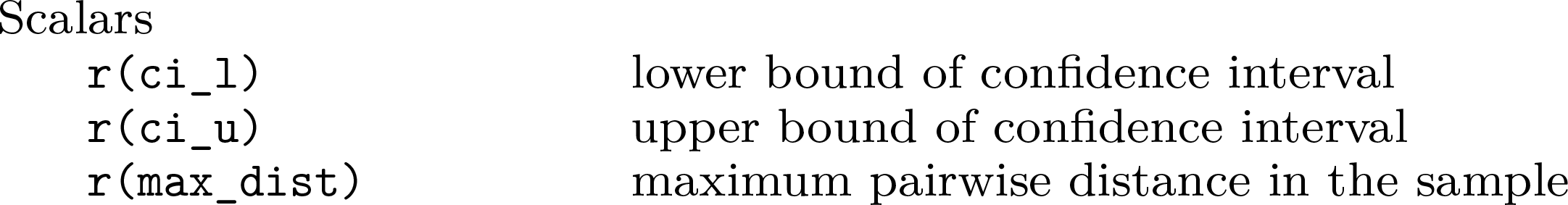
2.6.3 Stored results

spurtest stores the following in r():

2.7 Confidence sets for spatial half-life and the spurhalflife command

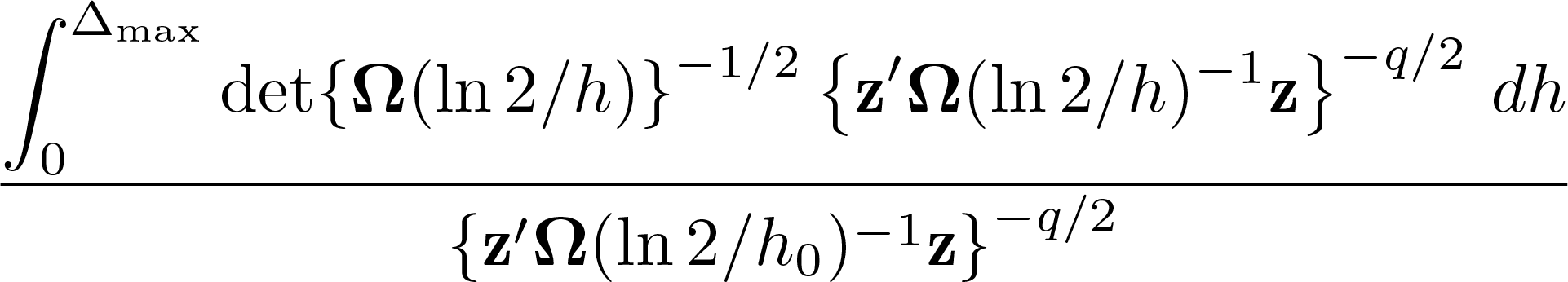
For completeness, we also implement a method proposed in Müller and Watson (2024) to construct confidence sets for the spatial half-life of a process, that is, the spatial distance at which the correlation in the process is equal to 1/2. In the LTU framework, this is directly connected to the parameter c. Specifically, the half-life h is equal to ln 2/c. Confidence intervals can then be constructed as the sets of values of h for which the null hypothesis H₀ : h₀ = h cannot be rejected. The test statistic suggested by Müller and Watson (2024), compares how well the data fit under H₀ to their average fit across a range [0, Δ_max] of alternative values of h, where Δ_max is the maximum pairwise distance of the sample locations, with the weighting chosen to be uniform in h. For a given h₀, a CV(h₀) for this test statistic can be computed using Monte Carlo simulation as described in section 2.2 by drawing from the null distribution z ∼ N{0, Ω(ln 2/h₀)} and computing the 1 — α quantile of the resulting distribution. Comparing the test statistic based on data with this CV yields a test of H₀ : h₀ = h. Repeating this for a grid of values h₀ and collecting all values that are not rejected then yields a 100(1 — α)% confidence set for h. For further details, see section 4.4 of Müller and Watson (2024).

2.7.1 Syntax

spurhalflife varname [if] [in] [, q(#) nrep(#) level(#) latlong normdist]

varname is the numerical variable whose spatial half-life is of interest.

The variables containing the spatial coordinates must be named s_1, s_2, …, s_p. (See explanation in section 2.6.)

2.7.2 Options

q(#) specifies the number of weighted averages to be used in the test. The default is q(15).

nrep(#) specifies the number of Monte Carlo draws to be used to simulate the distribution of the test statistic. The default is nrep(100000).

level(#) specifies the desired confidence level in percent. The default is level(95).

latlong specifies that the spatial coordinates are given in latitude (stored in s_1) and longitude (stored in s_2) (see above).

normdist specifies that the results be returned as fractions of the maximum pairwise distance in the sample. Otherwise, they are returned in meters (if latlong is specified) or the units of the original Euclidean coordinates (if latlong is not specified).

2.7.3 Stored results

spurhalflife stores the following in r():

3 Correction through spatial differencing and the spur- transform command

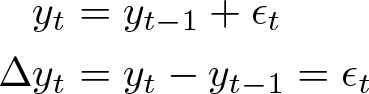
Having tested for and found evidence of the presence of spatial unit roots, the econometrician needs a way to correct for them to be able to estimate regression coefficients consistently. The standard approach in the time-series literature is to take first differences of the data:

\begin{aligned} y_{t} = y_{t - 1} + \in_{t} \\ Δ y_{t} = y_{t} - y_{t - 1} + \in_{t} \end{aligned}

This yields a stationary process that can be used in regressions. The equivalent transformation in the spatial context is not obvious: observations in space cannot be ordered in the way that a time series can and are unevenly spaced, so which value to subtract from each observation is not clear. Müller and Watson (2024) propose four possible linear transformations, the last of which they find to be the most powerful in their simulations. The following presents all four and illustrates their effects using the simulated LBM from section 2.1. Throughout, the vectors

y = (y_{1}, \dots, y_{n})

and

y * = (y_{1} *, \dots, y_{n} *)

refer to the raw and transformed data vectors, respectively. Furthermore,

H = I - H

refers to the respective transformation matrix, such that

y = H y = y - \tilde{H} y

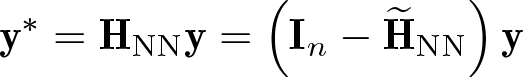
3.1 Nearest-neighbor differences

One obvious differencing procedure would be

y_{l} * = y_{l} - y_{ℓ (l)}

where

s_{ℓ (l)}

is the location nearest to s_l. This is equivalent to

y * = H_{NN} y = (I_{n} - {\tilde{H}}_{NN}) y

where

{\tilde{H}}_{N N, l j}

j = ℓ (l)

and 0 otherwise.

3.2 Isotropic differences

Instead of taking differences only with respect to the nearest neighbor (NN), another option would be to subtract the mean of all observations in a neighborhood of radius b:

y_{l} * = y_{l} - {\bar{y}}_{l} (b)

Where

\begin{aligned} {\bar{y}}_{l} (b) = \frac{1}{m_{l} (b)} \sum_{j \neq l} 1 [| s_{l} - s_{j} | < b] y_{j} \\ m_{l} (b) = \sum_{j \neq l} 1 [| s_{l} - s_{j} | < b] \end{aligned}

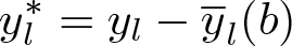
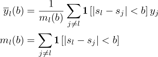
This is equivalent to

y * = H_{ISO} y = (I_{n} - {\tilde{H}}_{ISO}) y

where ${\tilde{H}}_{ISO, l j} = m_{l} {(b)}^{- 1} 1 [| s_{l} - s_{l} | < b] y_{j}$ for $j \neq 0$ and 0 for $j = l$ .

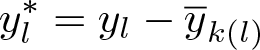
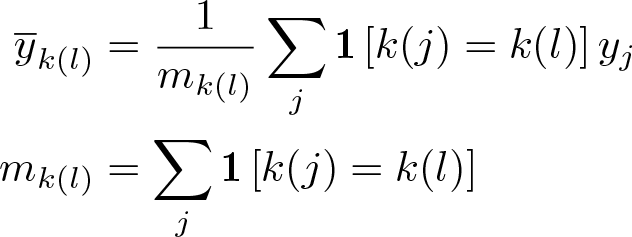
3.3 Clustered demeaning

A third option is to partition the data into K clusters and subtract the mean within its cluster from each observation (or, equivalently, including cluster fixed effects in the regressions). These clusters could be based on knowledge of the structure of the data (for example, states) or constructed through techniques like k-means clustering. The transformed data are then

y_{l} * = y_{l} - {\bar{y}}_{k} (l)

where

\begin{aligned} {\bar{y}}_{k} (l) = \frac{1}{m_{k} (l)} \sum_{j} 1 [k (j) = k (l)] y_{j} \\ m_{k} (l) = \sum_{j} 1 [k (j) = k (l)] \end{aligned}

and k(l) is the cluster that l belongs to. This is equivalent to

y * = H_{CL} y = (I_{n} - {\tilde{H}}_{CL}) y

where

{\tilde{H}}_{CL, l j} = m_{k (l)}^{- 1} 1 [k (j) = k (l)] y_{j}

3.4 LBM generalized least-squares transformation

The previous three transformations are ad hoc ways of correcting strong spatial dependence. Following their characterization of spatial unit-root processes as approximated by LBM, Müller and Watson (2024) propose a generalized least-squares (GLS) transformation based on the covariance matrix induced by LBM. Recall that under LBM, the demeaned data are distributed as y ∼ N(0,MƩ _L M). The standard GLS transform is then

\begin{aligned} y * = (M Σ_{L} M)^{- 1 / 2} y \\ \equiv H_{LBM - GLS} y \equiv (I_{n} - {\tilde{H}}_{LBM - GLS}) y \end{aligned}

where

(M Σ_{L} M)^{- 1 / 2}

is the Moore-Penrose inverse of

(M Σ_{L} M)^{- 1 / 2}

. To see how this transformation can be described as “spatial differencing”, it is useful to relate this back to the time-series case: it is easy to show that taking first differences of any evenly spaced time series is exactly equivalent to a (particular) GLS transformation based on the covariance matrix of a standard random walk. The LBM-GLS transformation translates this logic to the multidimensional spatial case, using the LBM covariance matrix. Figure 4 further illustrates the effects of the transformation.

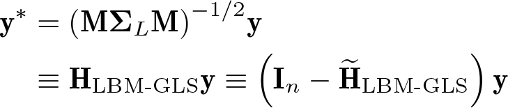
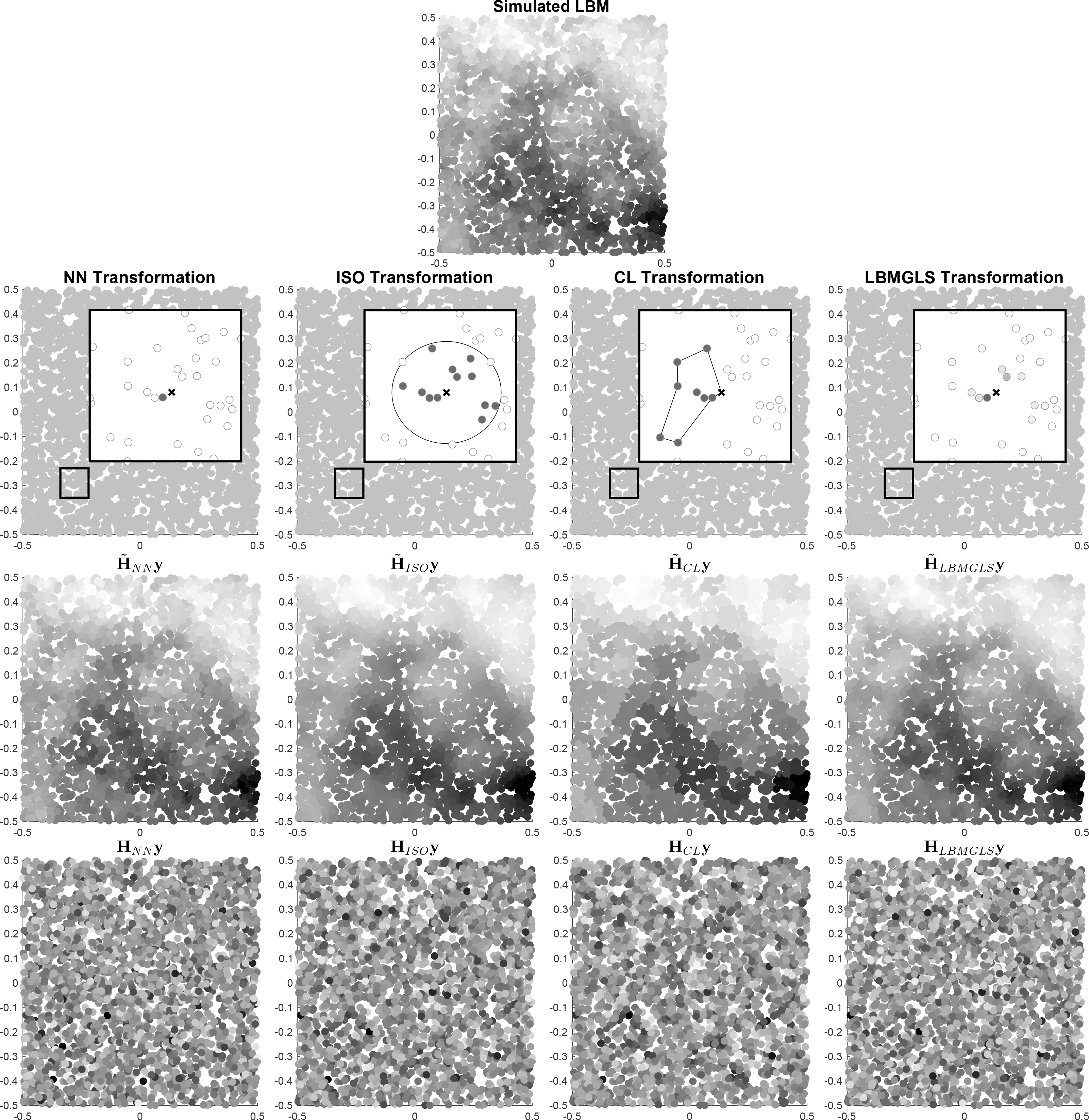
Figure 4 illustrates all four transformations. The single plot at the top is the “raw” data used for this illustration, which is the simulated LBM process from figure 3. The four columns below show the four described transformations. Within each column, the top panel illustrates the transformation for one focal data point (marked with x): the shaded dots are the data points whose weighted values are subtracted from the focal point, with a darker shade indicating a larger weight. In the NN transformation, only the closest neighbor is subtracted. In the isotropic and cluster transformations, an unweighted mean of surrounding observations is subtracted. The LBM-GLS transformation subtracts a weighted mean of all surrounding observations, with weights quickly decaying with distance. The middle panel shows the values that are subtracted from the raw data $(\tilde{H} y)$ , and the bottom panel shows the transformed data (Hy).⁹

3.5 Syntax

spurtransform varlist [if] [in], prefix(string) [transformation(string) radius(#) clustvar(varname) latlong replace separately]

varlist is the list of variables to be transformed. The transformed variables will be stored under the original variables’ names prefixed with prefix. If varlist contains several variables, they are all transformed using the same matrix H, meaning that only observations where all specified variables are nonmissing will be included. To override this behavior, specify the option separately.

The variables containing the spatial coordinates must be named s_1, s_2, …, s_p. (See explanation in section 2.6.)

3.6 Options

prefix(string) specifies the prefix for the variable names under which the transformed data will be stored. For example, when transforming the variable x, specifying prefix(”h_”) will result in the transformed variable to be stored as h_x. prefix() is required.

transformation(string) specifies the type of transformation. string must be one of lbmgls, nn, iso, or cluster. The default is transformation(lbmgls).

radius(#) specifies the radius in meters (if latlong is specified) or in the units of the original coordinates (if latlong is not specified), which are to be used for isotropic differencing (b in the notation above). This option is allowed only with transformation(iso).

clustvar(varname) specifies the variable that is to be used for clustering. This option is allowed only with transformation(cluster).

latlong specifies that the spatial coordinates are given in latitude (stored in s_1) and longitude (stored in s_2) (see above).

replace allows the command to overwrite variables when storing the transformed data.

separately executes the transformation separately for all variables in varlist. This leads to different results if there are missing observations in some variables because the default behavior is to construct the H matrix based only on those observations for which all variables are nonmissing.

4 Regression analysis using the M^ler-Watson approach

4.1 Proposed procedure

Having outlined the methods presented in Müller and Watson (2024) as well as our implementation thereof, we now turn to their practical application in regression analyses of spatial data. We propose a simple algorithm, summarized in figure 5:

Figure 5.

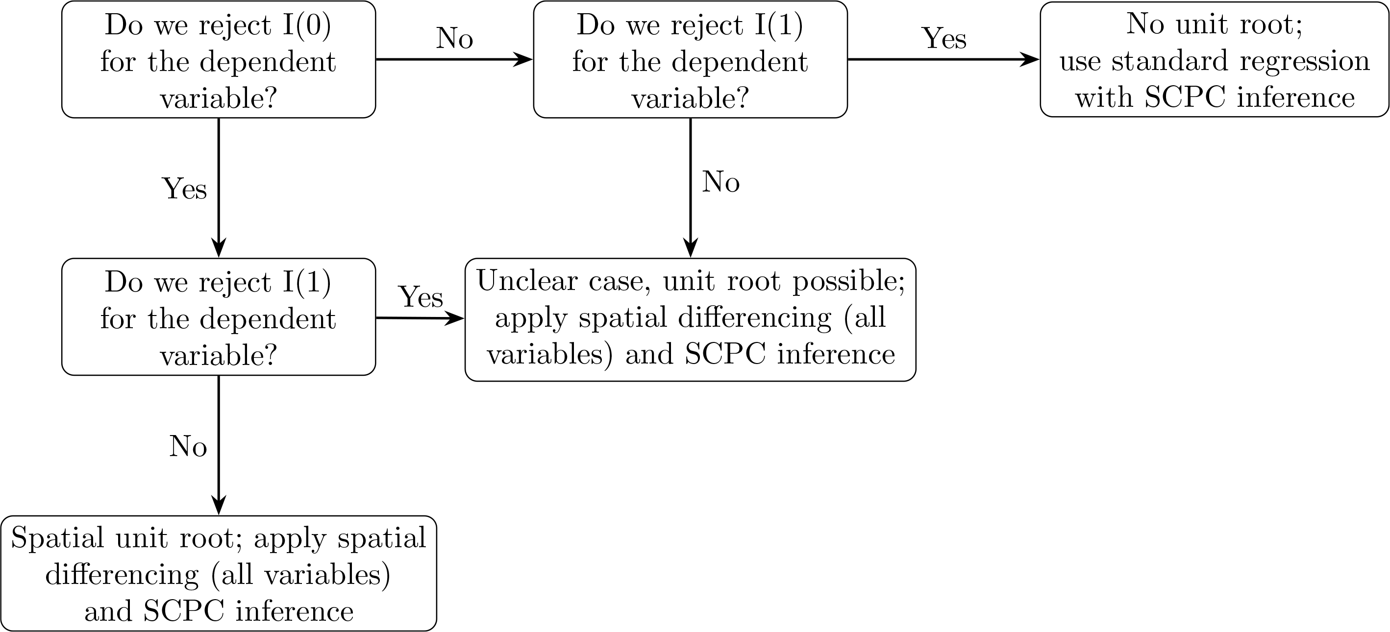
Flow diagram showing how to apply the Müller–Watson approach

We first test whether the dependent variable contains a unit root. To this end, we examine whether we can reject that it is I(0). If so, we test whether we can reject that it is I(1). If we cannot reject, a unit root is most likely present, and we need to apply one of the transformation methods discussed above to remove it. In this case, we propose differencing both the dependent and the independent variables for ease of interpretation of the regression coefficients. If we reject I(0) but also I(1), or neither, the case is indeterminate; it is arguably wise to difference and report results using transformed variables. If we do not reject the dependent variable being I(0) but can reject that it is I(1), we can confidently proceed without differencing. In all cases, regression inference still needs to account for any remaining (weak) spatial correlation; we suggest using the SCPC approach in Müller and Watson (2022, 2023).

Multivariate cases and instrumental variables can be handled analogously. Because the hypothesized relationship involves x and y, we should proceed with differencing all independent variables. Also, because instrumental-variables estimation represents a rescaling of the relationship between y and z via x, we can proceed analogously in this case.¹⁰

4.2 Illustration using Stata

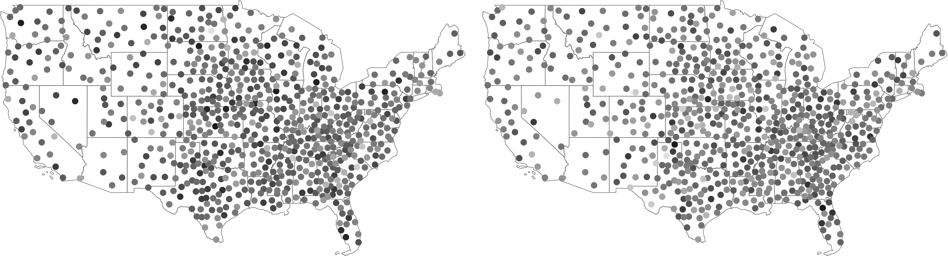
To illustrate this procedure and the use of our community-contributed commands, we simulate two independent LTU processes x and y with very high persistence (c = 0.01), using 722 US commuting zone centroids as locations. We take the location data from the replication package of Müller and Watson (2024), who obtained them from Chetty et al. (2014), and provide them in a supplementary file, example.dta, along with the simulated data.¹¹ This data file also includes further variables from Chetty et al. (2014), which we use in appendix A; however, here we require only the latitude and longitude variables s_1 and s_2 alongside y and x:

Figure 6 plots the simulated variables using the geoplot command (Jann 2023), the code for which we omit here for brevity but include in example_reg.do in the supplementary materials. The shade of each dot indicates the value of the respective variable at that location. Strong spatial dependence is clearly visible in both variables.

Running a simple regression of y on x and applying SCPC inference again illustrates the issue of spurious regression results in the presence of (near) unit roots: in this case, there is a strongly significant negative correlation between y and x, even though they are independent in population:

Figure 6.

Simulated dependent variable y (left) and independent variable x (right)

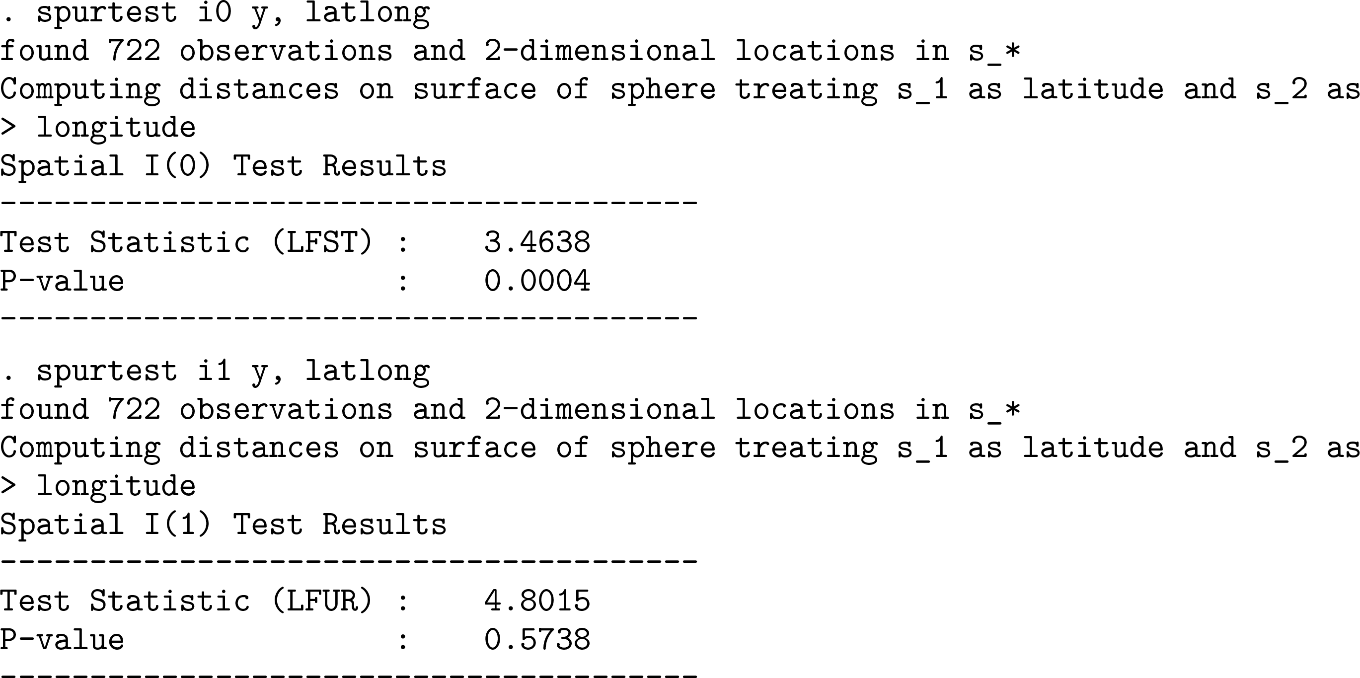
We now follow the procedure outlined above by applying the I(0) and I(1) tests to y using the spurtest command. We can reject that y is I(0) with very high confidence, and we cannot reject that it is I(1), indicating the presence of a unit root:

Therefore, we use spurtransform to difference both y and x using the LBM-GLS transformation, which adds the transformed variables h_y and h_x to the dataset. Figure 7 plots the transformed variables, now showing much less spatial dependence.

Figure 7.

Transformed dependent variable h_y (left) and independent variable h_x (right)

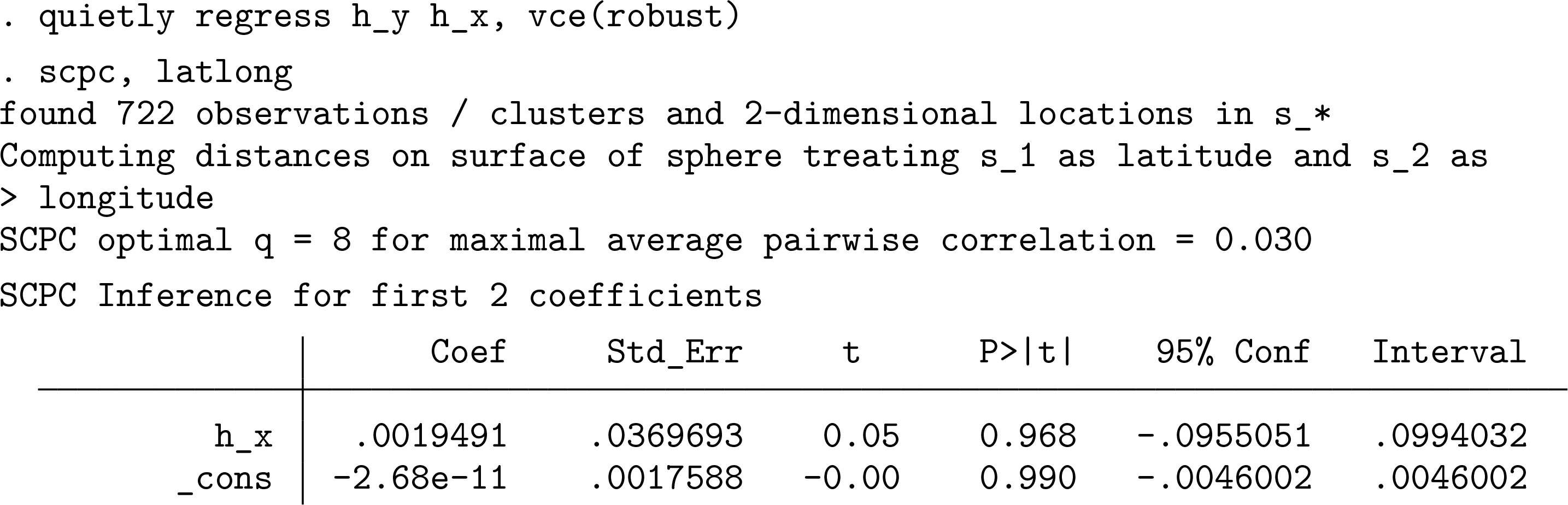
Finally, we run the regression of h_y on h_x and apply SCPC inference. The coefficient is now close to 0 and not statistically significant, showing that our procedure correctly diagnosed and corrected the spurious regression problem:

4.3 Monte Carlo simulations

We repeat the above exercise 200 times, each time simulating independent x and y processes as above. We omit the simulation code here for brevity but provide it in the supplementary materials as example_montecarlo.do. For each repetition, we draw the dependence parameters c_x and c_y from a log-normal distribution such that log(c _x ) ∼ N(3, 2) and log(c_y) ∼ N(3, 2), which yields a range of realistic persistence levels in this setting. We first estimate the uncorrected regression of y on x with SCPC inference, and then we apply our procedure to test for unit roots (with a 5% threshold for significance) and, if necessary, difference both variables before reestimating the regression with SCPC inference. Figure 8 summarizes the results. The left panel shows the estimated coefficients from the uncorrected and corrected regressions, respectively. The right panel shows the share of repetitions in which the null hypothesis of no effect is rejected at the 5% level. This shows that the correction substantially reduces the variance of the estimated coefficients around the true value of 0 and that it reduces the (false) rejection rate from over 10% to under 5%.

Figure 8.

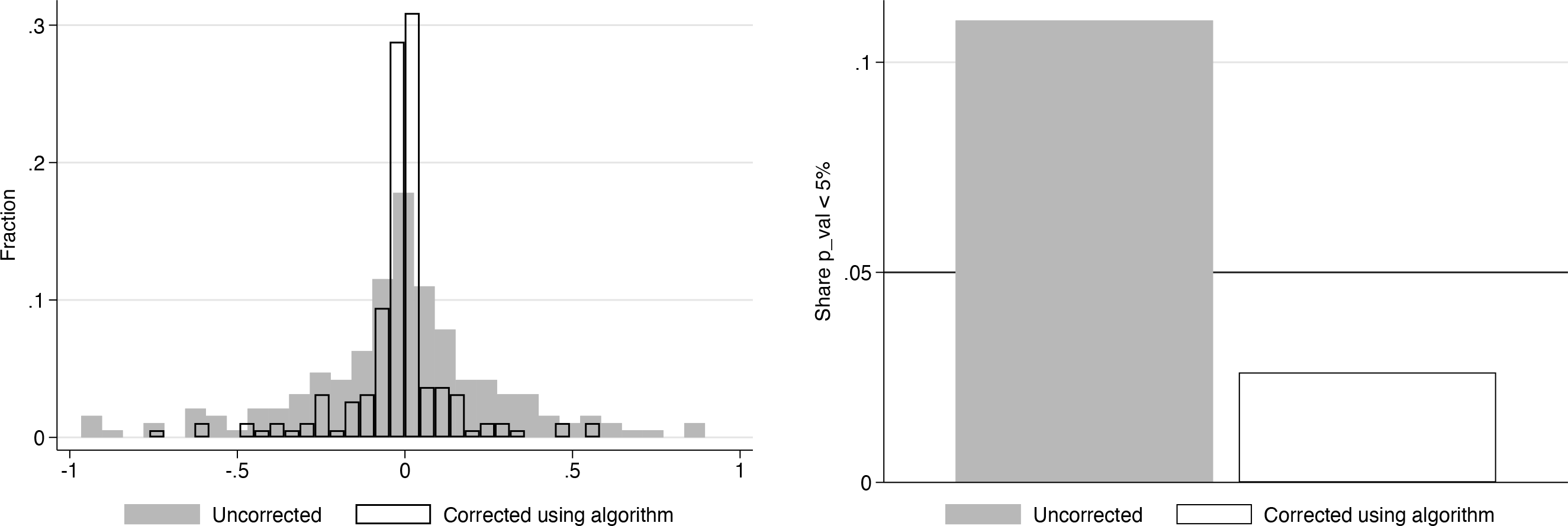
Simulation results: Estimated coefficients (left) and rejection shares at 5% level (right)

Conclusions

We presented spur, an implementation of newly developed econometric methods that help to diagnose and correct spatial unit roots (Müller and Watson 2024), and we discussed its use in regression analysis. How these new methods perform compared with alternative methods to correct for strong spatial dependence is an open question. In follow-up work, we plan to apply this approach as well as several alternatives to both simulated and observational data, examining their power and size properties. This will clarify when each method is best applied, given a particular setting.

Supplemental Material

sj-txt-1-stj-10.1177_1536867X261449932 - Supplemental material for Testing and correcting for spatial unit roots in regression analysis

Supplemental material, sj-txt-1-stj-10.1177_1536867X261449932 for Testing and correcting for spatial unit roots in regression analysis by Sascha O. Becker, P. David Boll and Hans-Joachim Voth in The Stata Journal

Supplemental Material

sj-pdf-1-stj-10.1177_1536867X261449932 - Supplemental material for Testing and correcting for spatial unit roots in regression analysis

Supplemental material, sj-pdf-1-stj-10.1177_1536867X261449932 for Testing and correcting for spatial unit roots in regression analysis by Sascha O. Becker, P. David Boll and Hans-Joachim Voth in The Stata Journal

Supplemental Material

sj-dta-2-stj-10.1177_1536867X261449932 - Supplemental material for Testing and correcting for spatial unit roots in regression analysis

Supplemental material, sj-dta-2-stj-10.1177_1536867X261449932 for Testing and correcting for spatial unit roots in regression analysis by Sascha O. Becker, P. David Boll and Hans-Joachim Voth in The Stata Journal

Supplemental Material

sj-dta-1-stj-10.1177_1536867X261449932 - Supplemental material for Testing and correcting for spatial unit roots in regression analysis

Supplemental material, sj-dta-1-stj-10.1177_1536867X261449932 for Testing and correcting for spatial unit roots in regression analysis by Sascha O. Becker, P. David Boll and Hans-Joachim Voth in The Stata Journal

Footnotes

Acknowledgments

The community-contributed code is based on the MATLAB code provided by Ulrich Muller and Mark Watson (). Our community- contributed code replicates the results in Müller and Watson (2024) based on their MATLAB code 1:1. Any errors in the community-contributed code remain our own. We are obliged to Ulrich Muller and Mark Watson for useful conversations and suggestions. We thank Daniel Gottlich and Elie Malhaire for excellent research assistance.

8 Programs and supplemental materials

To install the software files as they existed at the time of publication of this article, type

The latest version of the programs can be installed using

and (optional) example data and do-files can be downloaded using

Revised and improved versions of the programs may become available in the future at

https://github.com/pdavidboll/SPUR or on our webpages (

and https://pauldavidboll.com and ).

We provide example do-files and data to replicate the results in section 4 and appendix A. Please refer to the provided readme.txt file for further information.

Notes

About the authors

Sascha O. Becker is professor of economics at the University of Warwick, UK, and Xiaokai Yang Chair of Business and Economics at Monash University, Australia. He is also affiliated with CAGE, CEH@ANU, CEPH, CESifo, CReAM, CEPR, Ifo, IZA, ROA, RF Berlin, and SoDa Labs.

P. David Boll is a PhD candidate at the University of Warwick, UK.

Hans-Joachim Voth is UBS Foundation Professor of Economics, University of Zurich, Switzerland, and Scientific Director of the UBS Center for Economics in Society. He is also affiliated with CEPR and CAGE.

A Appendix: Reproducing the Chetty et al. (2014) results in Müller and Watson (2024)

To demonstrate that our community-contributed code works as expected, we reproduce table 1 in Müller and Watson (2024), which uses data from Chetty et al. (2014). These data are originally in .xlsx format and were obtained from the replication package accompanying Müller and Watson (2024). We read and clean these data in the script make_example_data.do and save the resulting dataset as example.dta. We keep their variable names one to one. The key outcome variable is called am (absolute mobility), whereas all other variables are predictors of the potential for absolute mobility, such as tlfpr, the teenage labor force participation rate. am and tlfpr are the two variables depicted in figure 1, panel (c). In what follows, we list the sequence of community- contributed commands that produces our table A1.

After this, we call the commands in the spur suite—spurtest, spurhalflife, and spurtransform—before finally applying the scpc command made available by Müller and Watson (2023) on their website. They apply the proper standard errors appropriate in the context of spatial autocorrelation on the (transformed) data.

We follow the exact same ordering of columns as Müller and Watson (2024) to allow for comparison of results of their original MATLAB code and our community-contributed code. Our results are shown in table A1. Apart from minor differences in the second decimal place, which are explained by the fact that the methods use simulations based on random numbers, our code reproduces the results in Müller and Watson (2024) exactly.

Note that in most cases, applying the LBM-GLS transformation does not turn significant results in levels into insignificant ones. While there are occasional cases like the effect of the manufacturing share or Chinese import growth (significant in levels but not after the transformation), where the new 95% confidence interval includes zero, these are rare. This is true despite the fact that the overwhelming majority of dependent variables appear to be I(1), exhibiting a strong form of spatial dependence.

References

Chetty

Hendren

Kline

Saez

. 2014. Where is the land of opportunity? The geography of intergenerational mobility in the United States. Quarterly Journal of Economics 129: 1553–1623. https: // doi.org /10.1093 /qje/ qju022.

Fingleton

. 1999. Spurious spatial regression: Some Monte Carlo results with a spatial unit root and spatial cointegration. Journal of Regional Science 39: 1–19. https: //doi.org/10.1111 /1467-9787.00121.

Granger

C. W. J.

Newbold

. 1974. Spurious regressions in econometrics. Journal of Econometrics 2: 111–120. 10.1016/0304-4076(74)90034-7.

Jann

2005. moremata: Stata module (Mata) to provide various functions. Statistical Software Components S455001, Department of Economics, Boston College. https://ideas.repec.org/c/boc/bocode/s455001.html.

. 2023. geoplot: Stata module to draw maps. Statistical Software Components S459211, Department of Economics, Boston College. https://ideas.repec.org/c/boc/ bocode / s459211.html.

King

M. L

. 1987. Towards a theory of point optimal testing. Econometric Reviews 6: 169–218. 10.1080/07474938708800129.

Muller

U. K.

Watson

M. W.

. 2008. Testing models of low-frequency variability. Econometrica 76: 979–1016. 10.3982/ECTA6814.

. 2019. Low-frequency analysis of economic time series. Working Papers 202013, Department of Economics, Princeton University. https://www.princeton.edu/∼umueller/HOE.pdf.

. 2022. Spatial correlation robust inference. Econometrica 90: 2901–2935. https://doi.org/10.3982/ECTA19465 .

10.

2023. Spatial correlation robust inference in linear regression and panel models. Journal of Business and Economic Statistics 41: 1050–1064. 10.1080/07350015.2022.2127737.

11.

. 2024. Spatial unit roots and spurious regression. Econometrica 92: 1661–1695. 10.3982/ECTA21654.

12.

Phillips

P. C. B

. 1986. Understanding spurious regressions in econometrics. Journal of Econometrics 33: 311–340. 10.1016/0304-4076(86)90001-1.

Supplementary Material

Please find the following supplemental material available below.

For Open Access articles published under a Creative Commons License, all supplemental material carries the same license as the article it is associated with.

For non-Open Access articles published, all supplemental material carries a non-exclusive license, and permission requests for re-use of supplemental material or any part of supplemental material shall be sent directly to the copyright owner as specified in the copyright notice associated with the article.

1.21 MB

0.00 MB

0.29 MB

7.03 MB

0.00 MB