Extreme Behaviors in Risk Measurement via Joint Tail-Based Cumulative Residual Entropy and Its Generalized Version

Abstract

Tail risk analysis plays a pivotal strategic role in risk management, particularly in light of economic crises. In this context, the purpose of this paper is to examine the asymptotic properties of Joint Tail-based Cumulative Residual Entropy ( $J T C R E$ ) in a bivariate setup involving two variables, $X$ and $Y$ . In this setup, $X$ is considered the variable of interest, while $Y$ serves as the benchmark variable. We provide a generalization of the Joint Tail-based Cumulative Residual Entropy to create a more flexible version that allows for a more comprehensive analysis of extreme risk. This generalization leads to a deeper understanding of the tail relationship between $X$ and $Y$ and their respective impacts on a specific system. To illustrate our results, we conducted the study under both tail-dependent and tail-independent scenarios. We supplemented our research with practical examples and applied our findings to real-world financial data, employing our proposed non-parametric estimator of $J T C R E$ as the basis for our analysis.

Keywords

joint tail-based cumulative residual entropy copulas tail dependence tail risk and variability heavy tails

1. Introduction

In academic research and scholarly literature, tail-based risk measures have been proposed to evaluate and investigate the tail risk of financial variables. These measures are primarily used to assess the risk of extreme events occurring in financial markets or other economic systems. The increasing frequency of financial crises, such as the 2008 Great Depression and the COVID-19 pandemic, in the last two decades has highlighted the need for researchers and practitioners to pay closer attention to extreme events and their potential impact on the financial industry (Gardes, 2022; Chen et al., 2023; Broda et al., 2018). These extreme events, often referred to as black swan events, can result in significant market volatility and widespread financial instability. Tail-based risk measurement allows researchers and practitioners to better understand the likelihood and potential severity of these events, enabling them to develop appropriate risk management strategies. By analyzing tail risk, financial institutions can identify weaknesses in their risk management processes and implement effective measures for black swan events.

In academic literature, several papers have been published to investigate the effects of financial risk and propose different approaches to address extreme risk and variability (El Qalli and Said, 2023). One such measure is Expected Shortfall ( $E S$ ), which is a coherent risk measure (see Artzner et al., 1999; Acerbi, 2002; Ben Hssain et al., 2024), such that for a loss random variable $X$ ,

E S_{p} (X) = E [X | X > V a R_{p} (X)],

(1)

where

V a R_{p} (X) = inf {x \in R | F_{X} (x) \geq p}

is the Value-at-Risk at a risk level

p \in (0, 1)

and

F_{X}

is the distribution function of

X

E S_{p}

has become increasingly popular in recent years due to its ability to capture both the severity and likelihood of tail events. However,

E S

is unable to fully capture the risk exposure that arises from the simultaneous movement of multiple variables (see Hou and Wang, 2019), particularly in relation to systemic risk. In response to this limitation, Acharya et al. (2017) recommended a generalized version of

E S

called Marginal Expected Shortfall (

M E S

), which is a conditional expectation, defined for a bivariate vector

(X, Y)

M E S_{p} (X; Y) = E [X | Y > Q_{Y} (1 - p)],

(2)

where

Q_{Y}

is the quantile function of

Y

. Throughout this paper, a random variable

X

(or

Y

) is used to model financial losses in cases where it takes positive values.

Mathematically speaking, regarding the exploration of tail heaviness using Extreme Value Theory, Cai et al. (2015) investigated the asymptotic behaviors of $M E S$ for quantifying the systemic risk associated with the anticipated loss when an extreme loss occurs in a specific financial sector. Additionally, Das and Fasen-Hartmann (2018) provides a non-parametric estimator of $M E S$ and investigates several other properties under asymptotic tail independence. However, according to Ji et al. (2021), $M E S$ overlooks the complete variation of a chosen random variable, which renders it unsuitable for researchers who aim to analyze such variability. In this context, Hou and Wang (2019) established the asymptotic limits for distortion risk measures. Specifically, for a non-negative random variable $X$ and a non-decreasing distortion function $g$ , where $g (0) = 0$ and $g (1) = 1$ , the distortion risk measure $ρ_{g} (X)$ is given as:

ρ_{g} (X) = \int_{0}^{\infty} g (1 - F_{X} (x)) d x .

(3)

Recently, Sun and Chen (2022) examined the extreme properties of the Tail Gini Functional (TGini) and the Joint Tail-Gini Functional (JTGini), introduced by Furman et al. (2017). These are defined for a bivariate random vector as

{TGini}_{p} (X; Y) = \frac{4}{p} Cov (X, F_{Y} (Y) ∣ F_{Y} (Y) > 1 - p),

(4)

and

{JTGini}_{p} (X; Y) = \frac{4}{p} Cov (X, F_{Y} (Y) ∣ X > Q_{X} (1 - p), Y > Q_{Y} (1 - p)),

(5)

where

Q_{X}

is the quantile function of

X

and

F_{Y}

is the distribution function of

Y

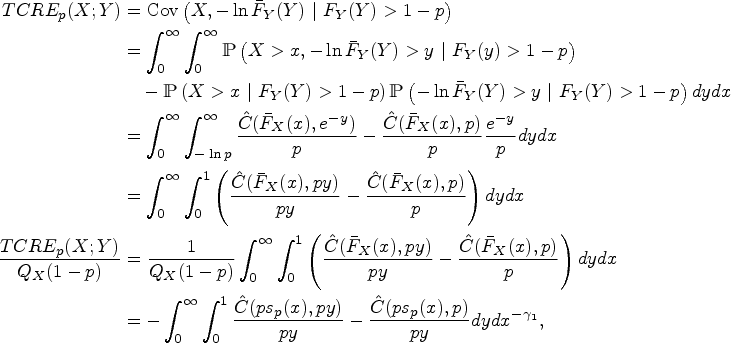
Despite the emergence of valuable tail risk concepts in the past decade, extending these ideas to numerous other important categories of risk measures remains challenging. One particularly important category is the entropy risk measures. Zuo and Yin (2023) provides the Choquet integral representation and discusses the coherent properties of various measures derived from entropy. Hu and Chen (2020) introduced Tail-based Cumulative Residual Entropy ( $T C R E$ ) in a univariate context, which was based on Cumulative Residual Entropy ( $C R E$ ) proposed by Rao et al. (2004). $T C R E$ can be defined, in terms of covariance, as follows:

T C R E_{p} (X) = Cov (X, - \ln {\bar{F}}_{X} (X) | F_{X} (X) > 1 - p),

(6)

where

{\bar{F}}_{X} = 1 - F_{X}

. Sun et al. (2022) introduces Tail-based Cumulative Residual Entropy in a bivariate context

(X, Y)

as a new approach to assess the variability of tail risk, defined as follows:

T C R E_{p} (X; Y) = Cov (X, - \ln {\bar{F}}_{Y} (Y) | F_{Y} (Y) > 1 - p),

(7)

In practical scenarios,

Y

represents a benchmark variable, such as the loss of a financial system or benchmark portfolio, while

X

is a variable to study, such as the loss of an individual asset or portfolio. It is worth noting that TCRE measures enable an overview of a monotonic relationship between

X

and

F_{Y} (Y)

, instead of a linear one as given by Gini type measures like TGini and JTGini.

In light of these existing papers, our contributions can be summarized as follows. We commence with the integration of the tail order property of the copula (Definition 2.2) as a degree of independence between two random variables in our context. This consideration enables us to examine situations where the tails of both $X$ and $Y$ can be regarded as either tail-dependent or tail-independent. Subsequently, we incorporate the tail of $X$ into the modeling process, resulting in a joint tail-oriented approach that encompasses both $X$ and $Y$ . This investigation has gained attention in recent literature (for example, in Ji et al. (2021)), then this paper aims to advance it further by exploring the asymptotic properties of Joint Tail-based Cumulative Residual Entropy (Definition 4.1) and its generalized version, which we introduce in Definition 4.3. This broader framework provides a more comprehensive examination of various dependence structures when studying extreme risk and variability.

The rest of the paper is organized as follows. In Section 2, we recall some concepts related to extreme value theory and tail dependence. Section 3 focuses on Tail-based Cumulative Residual Entropy. Section 4 introduces the asymptotic properties of Joint Tail-based Cumulative Residual Entropy, its generalization, and provides examples. Section 5 presents a real data analysis. The last section concludes.

2. Preliminaries

Throughout this paper, two positive functions $G_{1}$ and $G_{2}$ are said to be asymptotically equivalent if $lim_{ϵ \to ϵ_{0}} \frac{G_{1} (ϵ)}{G_{2} (ϵ)} = 1,$ where $ϵ_{0}$ typically represents either $0$ or $\infty$ . This equivalence is denoted by $G_{1} \sim G_{2}$ . Additionally, for any $(x, y) \in R^{2}$ , we define $x \land y$ as $min {x, y}$ .

2.1. Extreme Value Theory

Extreme value theory assumes that for a sequence of independent and identically distributed random variables ${X_{i}}_{i = 1}^{n}$ with a common distribution function $F$ , there are $σ_{n} > 0$ and $μ_{n} \in R$ such that

lim_{n \to \infty} P (σ_{n} (max {X_{1}, X_{2}, \dots, X_{n}} - μ_{n}) \leq x) = L_{γ} (x), x \in R .

with

L_{γ}

is a classical result given in Sklar (1959) as

L_{γ} (x) = e^{- (1 + γ x)^{- 1 / γ}}, 1 + γ x > 0.

where

γ \in R

, such that the regions

γ < 0

γ = 0

and

γ > 0

correspond to the Weibull, Gumbel, and Fréchet distributions, respectively. For the purposes of this paper, we focus on the case where

λ > 0

as our primary interest lies in heavy-tailed variables (i.e., the Fréchet case).

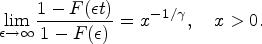
Suppose that the upper endpoint of the distribution $F$ is finite, and let $γ > 0$ , $F$ belongs to the domain of the Fréchet distribution if and only if:

lim_{ϵ \to \infty} \frac{1 - F (ϵ t)}{1 - F (ϵ)} = x^{- 1 / γ}, x > 0.

This indicates that the function

\bar{F}

is regularly varying at

\infty

with an index of

- 1 / γ

(refer to Bingham et al. (1989)). The definition of regular variation is as follows.

Definition 2.1
A measurable function $H : (0, \infty) \mapsto (0, \infty)$ is said to be regularly varying at $ϵ_{0} = 0$ or $\infty$ , with index $ν \in R$ if
$lim_{ϵ \to ϵ_{0}} \frac{H (ϵ x)}{H (ϵ)} = x^{ν}, x > 0,$
(8)
and we write $H \in {R V}_{ν} (ϵ_{0})$ . For simplicity, when $ϵ_{0} \equiv \infty$ , we use the notation $H \in {R V}_{ν}$ .

The theory of regular variation provides a significant mathematical framework for analyzing the asymptotic behavior of distribution function tails. This framework is particularly valuable in tail risk analysis and the quantification of tail variability.
2.2. Tail Dependence

As we aim to explore the tail independence between two variables, it is crucial to recall the concept of a two-dimensional copula, which quantifies the relationship between random variables. Throughout the paper, we consider two non-negative random variables $X$ and $Y$ with continuous distribution functions $F_{X} = 1 - {\bar{F}}_{X}$ and $F_{Y} = 1 - {\bar{F}}_{Y}$ . Then there exist a unique copulas, such that $C (F_{X} (x), F_{Y} (y)) = P (X \leq x, Y \leq y) for all (x, y) \in R^{2}$ (see Sklar, 1959). Then the survival copulas $\hat{C}$ satisfies

\hat{C} (v, u) = v + u - 1 + C (1 - v, 1 - u) for 0 \leq v, u \leq 1.

And we say

(X, Y)

follows a survival copulas

\hat{C}

\hat{C} ({\bar{F}}_{X} (x), {\bar{F}}_{Y} (y)) = P (X > x, Y > y)

for all

(x, y) \in R^{2}

To cover a broad range of dependence structures, including both tail-dependent and tail-independent cases, we revisit the definition of the tail order of a copula, aiming to assess the level of dependence (Hua and Joe, 2011). It can be verified that this tail order, denoted by $k$ , is equivalent to $\frac{1}{η}$ in Ledford and Tawn’s formulation, where $\frac{1}{2} \leq η \leq 1$ (Ledford and Tawn, 1996).

Definition 2.2
For $t \in [0, 1]$ , a factor $k > 0$ is said to be the tail order of $C$ if there exist $Ψ \in {R V}_{0} (0_{+})$ such that
$\hat{C} (t, t) \underset{t \to 0}{\sim} t^{k} Ψ (t) .$
(9)
For ease of reference, we utilize “tail order” specifically to denote the upper tail order.

The upcoming sections will present results under Assumption 2.3, which provides the foundational basis for the presented findings.
Assumption 2.3
$S_{1} :$
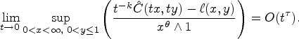
There exist $γ_{1} > 0$ , $θ_{1} < 0$ and a function $A$ with $lim_{t \to \infty} A (t) = 0$ such that
$lim_{t \to \infty} \frac{1}{A (1 / {\bar{F}}_{X} (t))} (\frac{{\bar{F}}_{X} (t x)}{{\bar{F}}_{X} (t)} - x^{- 1 / γ_{1}}) = x^{- 1 / γ_{1}} \frac{x^{θ_{1} / γ_{1}} - 1}{γ_{1} θ_{1}}, x > 0.$

$S_{2} :$
There exists a function $ℓ : (0, \infty)^{2} \to [0, \infty)$ and $θ > γ_{1}$ , $τ > 0$ , $1 \leq k \leq 2$ such that
$lim_{t \to 0} sup_{0 < x < \infty, 0 < y \leq 1} (\frac{t^{- k} \hat{C} (t x, t y) - ℓ (x, y)}{x^{θ} \land 1}) = O (t^{τ}) .$

$γ_{1}$ denotes the extreme value index that measures the heaviness of the right tail of $F_{X}$ . It is evident that as the parameter $1 / γ_{1}$ approaches zero, the distribution $F_{X}$ exhibits heavier tails.

Assumption $S_{1}$ holds true for a wide range of distribution functions (Haan and Ferreira, 2006) and denotes the second-order regular variation condition of the marginal distribution of $X$ .

Assumption $S_{2}$ defines a second-order condition for the tail dependence structure of $(X, Y)$ and is satisfied by various bivariate copulas (Nelsen, 2006). Therefore, the motivation behind these assumptions is that many different distribution functions, including Pareto and Fréchet distributions, satisfy them.
Remark 1
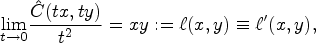
The function $ℓ (x, y)$ in hypothesis $S_{2}$ is important for capturing and representing the asymptotic behavior of $\hat{C} (t x, t y)$ as $t$ approaches zero. The function $ℓ$ satisfies $ℓ (p x, p y) = p^{k} ℓ (x, y)$ , indicating that $ℓ$ is $k$ -homogeneous. It naturally follows that $ℓ (x, 0) = ℓ (0, y) = ℓ (0, 0) = 0$ . In addition, for $k = 1$ , the function $ℓ$ coincides with the R-function, which has been used in recent literature (Asimit and Li, 2018; Das and Fasen-Hartmann, 2018). In this case, it can be considered as a simple transformation of the function $L$ defined in Haan and Ferreira (2006), such that for $x, y \geq 0$ ,
$L (x, y) = x + y - ℓ (x, y) .$
(10)
3. Tail-Based Cumulative Residual Entropy

In this section, we initially demonstrate the significance of generalizing result presented in Sun et al. (2022) through the incorporation of the tail order. Let ${\bar{F}}_{X} \in {R V}_{- 1 / γ_{1}}$ , and assume the limit in equation (11) exists

lim_{t \to 0} \frac{\hat{C} (t x, t y)}{t} := R (x, y), (x, y) \in (0, \infty) \times [0, 1),

(11)

in this case, the following asymptotic behavior have demonstrated by Sun et al. (2022),

lim_{p \to 0} \frac{T C R E_{p} (X; Y)}{Q_{X} (1 - p)} = \frac{γ_{1}}{1 - γ_{1}} \int_{0}^{\infty} R (x^{- 1 / γ_{1}}, 1) d x,

(12)

The tail order of a copula, given in Definition 2.2, captures the degree of dependence between random variables, as shown by Hua and Joe (2011). In equation (11) the tail order is taken such that

k = 1

which is not very useful for the cases where

X

and

Y

are tail independent. Thus, throughout the paper, we take

1 \leq k \leq 2

as we will focus on both situations where

X

and

Y

can be considered tail independent

(1 < k \leq 2)

or tail dependent

(k = 1)

. Furthermore, this means we only focus on positive dependence where:

P (X > x, Y > y) \geq P (X > x) P (Y > y), for all (x, y) \in R^{2} .

For more details we refer to Li and Li (2013) and Hua and Joe (2011).

Theorem 3.1

For a bivariate continuous non-negative random vector $(X, Y)$ with survival copula $\hat{C}$ , let $γ_{1} \in (0, 1)$ and suppose Assumptions $S_{1}$ and $S_{2}$ hold. If $\int_{0}^{\infty} ℓ (x^{- 1 / γ_{1}}, 1) d x < \infty$ , and $1 + γ_{1} - k > 0$ , then we have

lim_{p \to 0} \frac{T C R E_{p} (X; Y)}{p^{k - 1} Q_{X} (1 - p)} = \frac{1 + γ_{1} - k}{k - γ_{1}} \int_{0}^{\infty} ℓ (x^{- 1 / γ_{1}}, 1) d x .

(13)

Proof.

Define: $s_{p} (x) := \frac{{\bar{F}}_{X} (Q_{X} (1 - p) x^{- γ_{1}})}{p}, x \in (0, \infty)$ . Assumptions $S_{1}$ and $S_{2}$ imply that

lim_{p \to 0} \frac{\hat{C} (p s_{p} (x), p y)}{p^{k}} = ℓ (x, y), (x, y) \in (0, \infty) \times (0, 1] .

(14)

For two non-negative random variables

X

Y

with finite variances, we have

\begin{aligned} Cov (X; Y) & = \int_{0}^{\infty} \int_{0}^{\infty} (F_{X Y} (x, y) - F_{X} (x) F_{Y} (y)) d x d y \end{aligned}

(15)

\begin{aligned} = \int_{0}^{\infty} \int_{0}^{\infty} ({\bar{F}}_{X Y} (x, y) - {\bar{F}}_{X} (x) {\bar{F}}_{Y} (y)) d x d y, \end{aligned}

(16)

where

F_{X Y}

F_{X}

F_{Y}

are the joint and marginal distributions of

X

Y

, respectively, and

{\bar{F}}_{X Y}

{\bar{F}}_{X}

{\bar{F}}_{Y}

are survival ones. Thus,

\begin{aligned} T C R E_{p} (X; Y) & = Cov (X, - \ln {\bar{F}}_{Y} (Y) | F_{Y} (Y) > 1 - p) \\ = \int_{0}^{\infty} \int_{0}^{\infty} P (X > x, - \ln {\bar{F}}_{Y} (Y) > y | F_{Y} (y) > 1 - p) \\ - P (X > x | F_{Y} (Y) > 1 - p) P (- \ln {\bar{F}}_{Y} (Y) > y | F_{Y} (Y) > 1 - p) d y d x \\ = \int_{0}^{\infty} \int_{- \ln p}^{\infty} \frac{\hat{C} ({\bar{F}}_{X} (x), e^{- y})}{p} - \frac{\hat{C} ({\bar{F}}_{X} (x), p)}{p} \frac{e^{- y}}{p} d y d x \\ = \int_{0}^{\infty} \int_{0}^{1} (\frac{\hat{C} ({\bar{F}}_{X} (x), p y)}{p y} - \frac{\hat{C} ({\bar{F}}_{X} (x), p)}{p}) d y d x \\ \frac{T C R E_{p} (X; Y)}{Q_{X} (1 - p)} & = \frac{1}{Q_{X} (1 - p)} \int_{0}^{\infty} \int_{0}^{1} (\frac{\hat{C} ({\bar{F}}_{X} (x), p y)}{p y} - \frac{\hat{C} ({\bar{F}}_{X} (x), p)}{p}) d y d x \\ = - \int_{0}^{\infty} \int_{0}^{1} \frac{\hat{C} (p s_{p} (x), p y)}{p y} - \frac{\hat{C} (p s_{p} (x), p)}{p y} d y d x^{- γ_{1}}, \end{aligned}

where the last step is due to a change in variables. From Appendix A (equations (33) and (32)) we have

\int_{0}^{\infty} \int_{0}^{1} (\frac{s_{p} (x)}{y}) \land 1 d y d x^{- γ_{1}} < \infty and \int_{0}^{\infty} \int_{0}^{1} s_{p} (x) \land 1 d y d x^{- γ_{1}} < \infty .

(17)

Then, according to Theorem 2.2.3 in Nelsen (2006) we conclude

\int_{0}^{\infty} \int_{0}^{1} | \frac{\hat{C} (p s_{p} (x), p y)}{p y} - \frac{\hat{C} (p s_{p} (x), p)}{p} | d y d x^{- γ_{1}} \leq \int_{0}^{\infty} \int_{0}^{1} (\frac{s_{p} (x)}{y}) \land 1 + s_{p} (x) \land 1 d y d x^{- γ_{1}} < \infty .

(18)

Now, by applying the Dominated Convergence Theorem, we have that

\begin{aligned} lim_{p \to 0} \frac{T C R E_{p} (X; Y)}{p^{k - 1} Q_{X} (1 - p)} & = - \int_{0}^{\infty} \int_{0}^{1} lim_{p \to 0} \frac{\hat{C} (p s_{p} (x), p y)}{p^{k} y} - lim_{p \to 0} \frac{\hat{C} (p s_{p} (x), p)}{p^{k}} d y d x^{- 1 / γ_{1}} \\ = \int_{0}^{\infty} \int_{0}^{1} \frac{ℓ (x^{- 1 / γ_{1}}, y)}{y} d y d x - \int_{0}^{\infty} \int_{0}^{1} ℓ (x^{- 1 / γ_{1}}, 1) d y d x \\ = \int_{0}^{\infty} \int_{0}^{1} y^{k - 1} ℓ (\frac{x^{- 1 / γ_{1}}}{y}, 1) d y d x - \int_{0}^{\infty} ℓ (x^{- 1 / γ_{1}}, 1) d x \\ = \int_{0}^{\infty} \int_{0}^{1} y^{k - γ_{1} - 1} ℓ (x^{- 1 / γ_{1}}, 1) d y d x - \int_{0}^{\infty} ℓ (x^{- 1 / γ_{1}}, 1) d x \\ = \frac{1 + γ_{1} - k}{k - γ_{1}} \int_{0}^{\infty} ℓ (x^{- 1 / γ_{1}}, 1) d x, \end{aligned}

which completes the proof.

Remark 2

Note that for $k = 1$ the result of Theorem 3.1 coincide with the finding of Theorem 3.1 in Sun et al. (2022).

4. Joint Tail-Based Cumulative Residual Entropy

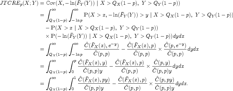
This section investigates the asymptotic properties of Joint Tail-based Cumulative Residual Entropy (JTCRE), given in Definition 4.1. We consider the extreme region defined by $X > Q (1 - p)$ and $Y > Q_{Y} (1 - p)$ for small values of $p$ , implying that both $X$ and $Y$ reside in their respective tail regions (see Asimit and Li, 2018). This framework allows JTCRE to capture the dependence between the upper tails of $X$ and $Y$ , potentially leading to a more accurate assessment of their extreme dependence. Moreover, we propose a generalization of JTCRE along with the introduction of its asymptotic result.

Definition 4.1 (Sun et al. (2022))

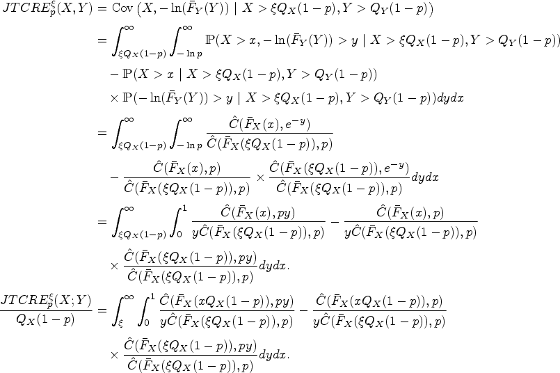
The Joint Tail-based Cumulative Residual Entropy is defined for a bivariate random variable $(X, Y)$ as follows:

J T C R E_{p} (X; Y) = Cov (X, - \ln ({\bar{F}}_{Y} (Y)) | X > Q_{X} (1 - p), Y > Q_{Y} (1 - p)) .

(19)

JTCRE is particularly useful in an economic context, especially in risk management and portfolio optimization, as it enables modeling the tail dependency between two variables. This can be interpreted as the way in which the extreme values of one variable, such as a financial asset, are related to the extreme values of another variable, such as a benchmark portfolio.

Theorem 4.2

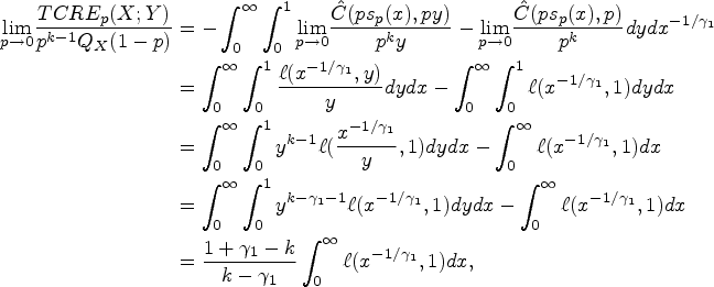
For a bivariate continuous non-negative random vector $(X, Y)$ with survival copula $\hat{C}$ , let $γ_{1} \in (0, 1)$ and suppose Assumptions $S_{1}$ and $S_{2}$ hold. Then we have

lim_{p \to 0} \frac{J T C R E_{p} (X; Y)}{Q_{X} (1 - p)} = \int_{1}^{\infty} \int_{0}^{1} \frac{ℓ^{'} (x^{- 1 / γ_{1}}, y)}{y} - \frac{ℓ^{'} (x^{- 1 / γ_{1}}, 1)}{y} ℓ^{'} (1, y) d y d x,

(20)

where

ℓ^{'} (x, y) = ℓ (x, y) / ℓ (1, 1)

Proof.

\begin{aligned} J T C R E_{p} (X; Y) & = Cov (X, - \ln ({\bar{F}}_{Y} (Y)) | X > Q_{X} (1 - p), Y > Q_{Y} (1 - p)) \\ = \int_{Q_{X} (1 - p)}^{\infty} \int_{- \ln p}^{\infty} P (X > x, - \ln ({\bar{F}}_{Y} (Y)) > y | X > Q_{X} (1 - p), Y > Q_{Y} (1 - p)) \\ - P (X > x | X > Q_{X} (1 - p), Y > Q_{Y} (1 - p)) \\ \times P (- \ln ({\bar{F}}_{Y} (Y)) | X > Q_{X} (1 - p), Y > Q_{Y} (1 - p)) d y d x \\ = \int_{Q_{X} (1 - p)}^{\infty} \int_{- \ln p}^{\infty} \frac{\hat{C} ({\bar{F}}_{X} (x), e^{- y})}{\hat{C} (p, p)} - \frac{\hat{C} ({\bar{F}}_{X} (x), p)}{\hat{C} (p, p)} \times \frac{\hat{C} (p, e^{- y})}{\hat{C} (p, p)} d y d x \\ = \int_{Q_{X} (1 - p)}^{\infty} \int_{0}^{p} \frac{\hat{C} ({\bar{F}}_{X} (x), y)}{\hat{C} (p, p) y} - \frac{\hat{C} ({\bar{F}}_{X} (x), p)}{\hat{C} (p, p)} \times \frac{\hat{C} (p, y)}{\hat{C} (p, p) y} d y d x \\ = \int_{Q_{X} (1 - p)}^{\infty} \int_{0}^{1} \frac{\hat{C} ({\bar{F}}_{X} (x), p y)}{\hat{C} (p, p) y} - \frac{\hat{C} ({\bar{F}}_{X} (x), p)}{\hat{C} (p, p)} \times \frac{\hat{C} (p, p y)}{\hat{C} (p, p) y} d y d x . \end{aligned}

Thus,

\frac{J T C R E_{p} (X; Y)}{Q_{X} (1 - p)} = - \int_{0}^{1} \int_{0}^{1} \frac{\hat{C} (p s_{p} (x), p y)}{\hat{C} (p, p) y} - \frac{\hat{C} (p s_{p} (x), p)}{\hat{C} (p, p)} \times \frac{\hat{C} (p, p y)}{\hat{C} (p, p) y} d y d x^{- γ_{1}} .

(21)

By Theorem 2.2.3 in Nelsen (2006), for

(x, y) \in (0, 1) \times (0, 1)

we have that

| \frac{\hat{C} (p s_{p} (x), p y)}{\hat{C} (p, p) y} - \frac{\hat{C} (p s_{p} (x), p)}{\hat{C} (p, p)} \times \frac{\hat{C} (p, p y)}{\hat{C} (p, p) y} | \leq \frac{p}{\hat{C} (p, p)} (\frac{s_{p} (x)}{y} \land 1) + {(\frac{p}{\hat{C} (p, p)})}^{2} (s_{p} (x) \land 1) .

Moreover, the findings in Appendix A indicate that

\int_{0}^{1} \int_{0}^{1} (\frac{p}{\hat{C} (p, p)} (\frac{s_{p} (x)}{y} \land 1) + {(\frac{p}{\hat{C} (p, p)})}^{2} (s_{p} (x) \land 1)) d y d x^{- γ_{1}} < \infty .

Consequently,

\int_{0}^{1} \int_{0}^{1} | \frac{\hat{C} (p s_{p} (x), p y)}{\hat{C} (p, p) y} - \frac{\hat{C} (p s_{p} (x), p)}{\hat{C} (p, p)} \times \frac{\hat{C} (p, p y)}{\hat{C} (p, p) y} | d y d x^{- γ_{1}} < \infty .

Assumptions

S_{1}

and

S_{2}

imply that

lim_{p \to 0} \frac{\hat{C} (p s_{p} (x), p y)}{\hat{C} (p, p)} = \frac{ℓ (x, y)}{ℓ (1, 1)} = ℓ^{'} (x, y), (x, y) \in (0, \infty) \times (0, 1] .

(22)

By applying the Dominated Convergence Theorem we obtain

\begin{aligned} lim_{p \to 0} \frac{T J C R E_{p} (X, Y)}{Q_{X} (1 - p)} & = - \int_{0}^{1} \int_{0}^{1} \frac{ℓ^{'} (x, y)}{y} - \frac{ℓ^{'} (x, 1)}{y} ℓ^{'} (1, y) d y d x^{- γ_{1}} \\ = \int_{1}^{\infty} \int_{0}^{1} \frac{ℓ^{'} (x^{- 1 / γ_{1}}, y)}{y} - \frac{ℓ^{'} (x^{- 1 / γ_{1}}, 1)}{y} ℓ^{'} (1, y) d y d x, \end{aligned}

this completes the proof.

Remark 3

A comparison of Theorems 3.1 and 4.2 reveals that incorporating the tail behavior of $X$ enriches the analysis. This inclusion provides deeper insights into the asymptotic behaviors observed, leading to a more comprehensive understanding.

4.1. Generalization of Joint Tail-Based Cumulative Residual Entropy

In real-world investments, it is clear that individuals exhibit varying decision-making processes due to differences in their levels of risk aversion (see Berkhouch et al., 2018). To address this diversity, in Definition 4.3 we propose a generalized version of the Joint Tail-based Cumulative Residual Entropy by considering a constant $0 < ξ \leq 1$ , which will allow more flexibility in risk measurement.

Definition 4.3
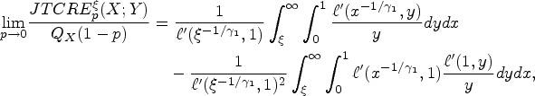
Let $0 < ξ \leq 1$ for a bivariate random variable $(X, Y)$ we further define a generalization of Joint Tail-based cumulative residual entropy:
$J T C R E_{p}^{ξ} (X, Y) = Cov (X, - \ln ({\bar{F}}_{Y} (Y)) | X > ξ Q_{X} (1 - p), Y > Q_{Y} (1 - p))$
(23)
Theorem 4.4
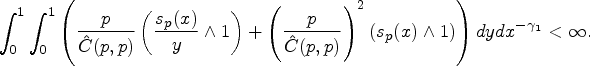
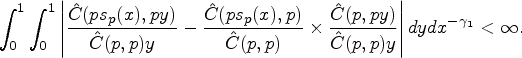
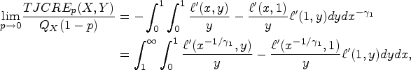
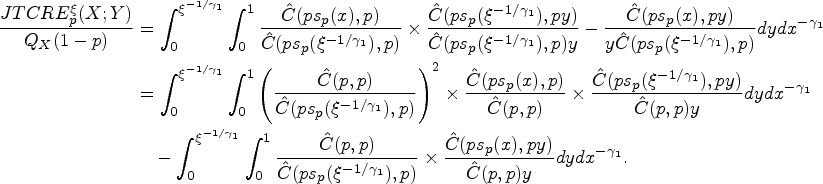
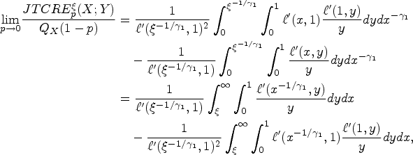
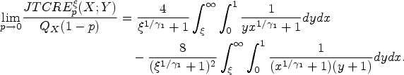
For a bivariate continuous non-negative random vector $(X, Y)$ with survival copula $\hat{C}$ , let $γ_{1} \in (0, 1)$ and suppose Assumptions $S_{1}$ and $S_{2}$ hold. Then we have for $0 < ξ \leq 1$ ,
$\begin{aligned} lim_{p \to 0} \frac{J T C R E_{p}^{ξ} (X; Y)}{Q_{X} (1 - p)} & = \frac{1}{ℓ^{'} (ξ^{- 1 / γ_{1}}, 1)} \int_{ξ}^{\infty} \int_{0}^{1} \frac{ℓ^{'} (x^{- 1 / γ_{1}}, y)}{y} d y d x \\ - \frac{1}{ℓ^{'} (ξ^{- 1 / γ_{1}}, 1)^{2}} \int_{ξ}^{\infty} \int_{0}^{1} ℓ^{'} (x^{- 1 / γ_{1}}, 1) \frac{ℓ^{'} (1, y)}{y} d y d x, \end{aligned}$
where $ℓ^{'} (x, y) = ℓ (x, y) / ℓ (1, 1)$ .
Proof.

$\begin{aligned} J T C R E_{p}^{ξ} (X, Y) & = Cov (X, - \ln ({\bar{F}}_{Y} (Y)) | X > ξ Q_{X} (1 - p), Y > Q_{Y} (1 - p)) \\ = \int_{ξ Q_{X} (1 - p)}^{\infty} \int_{- \ln p}^{\infty} P (X > x, - \ln ({\bar{F}}_{Y} (Y)) > y | X > ξ Q_{X} (1 - p), Y > Q_{Y} (1 - p)) \\ - P (X > x | X > ξ Q_{X} (1 - p), Y > Q_{Y} (1 - p)) \\ \times P (- \ln ({\bar{F}}_{Y} (Y)) > y | X > ξ Q_{X} (1 - p), Y > Q_{Y} (1 - p)) d y d x \\ = \int_{ξ Q_{X} (1 - p)}^{\infty} \int_{- \ln p}^{\infty} \frac{\hat{C} ({\bar{F}}_{X} (x), e^{- y})}{\hat{C} ({\bar{F}}_{X} (ξ Q_{X} (1 - p)), p)} \\ - \frac{\hat{C} ({\bar{F}}_{X} (x), p)}{\hat{C} ({\bar{F}}_{X} (ξ Q_{X} (1 - p)), p)} \times \frac{\hat{C} ({\bar{F}}_{X} (ξ Q_{X} (1 - p)), e^{- y})}{\hat{C} ({\bar{F}}_{X} (ξ Q_{X} (1 - p)), p)} d y d x \\ = \int_{ξ Q_{X} (1 - p)}^{\infty} \int_{0}^{1} \frac{\hat{C} ({\bar{F}}_{X} (x), p y)}{y \hat{C} ({\bar{F}}_{X} (ξ Q_{X} (1 - p)), p)} - \frac{\hat{C} ({\bar{F}}_{X} (x), p)}{y \hat{C} ({\bar{F}}_{X} (ξ Q_{X} (1 - p)), p)} \\ \times \frac{\hat{C} ({\bar{F}}_{X} (ξ Q_{X} (1 - p)), p y)}{\hat{C} ({\bar{F}}_{X} (ξ Q_{X} (1 - p)), p)} d y d x . \\ \frac{J T C R E_{p}^{ξ} (X; Y)}{Q_{X} (1 - p)} & = \int_{ξ}^{\infty} \int_{0}^{1} \frac{\hat{C} ({\bar{F}}_{X} (x Q_{X} (1 - p)), p y)}{y \hat{C} ({\bar{F}}_{X} (ξ Q_{X} (1 - p)), p)} - \frac{\hat{C} ({\bar{F}}_{X} (x Q_{X} (1 - p)), p)}{y \hat{C} ({\bar{F}}_{X} (ξ Q_{X} (1 - p)), p)} \\ \times \frac{\hat{C} ({\bar{F}}_{X} (ξ Q_{X} (1 - p)), p y)}{\hat{C} ({\bar{F}}_{X} (ξ Q_{X} (1 - p)), p)} d y d x . \end{aligned}$
Note that
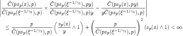
$\begin{aligned} \frac{J T C R E_{p}^{ξ} (X; Y)}{Q_{X} (1 - p)} & = \int_{0}^{ξ^{- 1 / γ_{1}}} \int_{0}^{1} \frac{\hat{C} (p s_{p} (x), p)}{\hat{C} (p s_{p} (ξ^{- 1 / γ_{1}}), p)} \times \frac{\hat{C} (p s_{p} (ξ^{- 1 / γ_{1}}), p y)}{\hat{C} (p s_{p} (ξ^{- 1 / γ_{1}}), p) y} - \frac{\hat{C} (p s_{p} (x), p y)}{y \hat{C} (p s_{p} (ξ^{- 1 / γ_{1}}), p)} d y d x^{- γ_{1}} \\ = \int_{0}^{ξ^{- 1 / γ_{1}}} \int_{0}^{1} {(\frac{\hat{C} (p, p)}{\hat{C} (p s_{p} (ξ^{- 1 / γ_{1}}), p)})}^{2} \times \frac{\hat{C} (p s_{p} (x), p)}{\hat{C} (p, p)} \times \frac{\hat{C} (p s_{p} (ξ^{- 1 / γ_{1}}), p y)}{\hat{C} (p, p) y} d y d x^{- γ_{1}} \\ - \int_{0}^{ξ^{- 1 / γ_{1}}} \int_{0}^{1} \frac{\hat{C} (p, p)}{\hat{C} (p s_{p} (ξ^{- 1 / γ_{1}}), p)} \times \frac{\hat{C} (p s_{p} (x), p y)}{\hat{C} (p, p) y} d y d x^{- γ_{1}} . \end{aligned}$
By Theorem 2.2.3 in Nelsen (2006) and Appendix A, for $(x, y) \in (0, 1) \times (0, 1)$ we have that
$\begin{aligned} | \frac{\hat{C} (p s_{p} (x), p)}{\hat{C} (p s_{p} (ξ^{- 1 / γ_{1}}), p)} \times \frac{\hat{C} (p s_{p} (ξ^{- 1 / γ_{1}}), p y)}{\hat{C} (p s_{p} (ξ^{- 1 / γ_{1}}), p) y} - \frac{\hat{C} (p s_{p} (x), p y)}{y \hat{C} (p s_{p} (ξ^{- 1 / γ_{1}}), p)} | \\ \leq \frac{p}{\hat{C} (p s_{p} (ξ^{- 1 / γ_{1}}), p)} (\frac{s_{p} (x)}{y} \land 1) + {(\frac{p}{\hat{C} (p s_{p} (ξ^{- 1 / γ_{1}}), p)})}^{2} (s_{p} (x) \land 1) < \infty . \end{aligned}$
Hence, by Assumptions $S_{1}$ and $S_{2}$ and the application of the Dominated Convergence Theorem, we conclude
$\begin{aligned} lim_{p \to 0} \frac{J T C R E_{p}^{ξ} (X; Y)}{Q_{X} (1 - p)} & = \frac{1}{ℓ^{'} (ξ^{- 1 / γ_{1}}, 1)^{2}} \int_{0}^{ξ^{- 1 / γ_{1}}} \int_{0}^{1} ℓ^{'} (x, 1) \frac{ℓ^{'} (1, y)}{y} d y d x^{- γ_{1}} \\ - \frac{1}{ℓ^{'} (ξ^{- 1 / γ_{1}}, 1)} \int_{0}^{ξ^{- 1 / γ_{1}}} \int_{0}^{1} \frac{ℓ^{'} (x, y)}{y} d y d x^{- γ_{1}} \\ = \frac{1}{ℓ^{'} (ξ^{- 1 / γ_{1}}, 1)} \int_{ξ}^{\infty} \int_{0}^{1} \frac{ℓ^{'} (x^{- 1 / γ_{1}}, y)}{y} d y d x \\ - \frac{1}{ℓ^{'} (ξ^{- 1 / γ_{1}}, 1)^{2}} \int_{ξ}^{\infty} \int_{0}^{1} ℓ^{'} (x^{- 1 / γ_{1}}, 1) \frac{ℓ^{'} (1, y)}{y} d y d x, \end{aligned}$
this completes the proof.
4.2. Examples

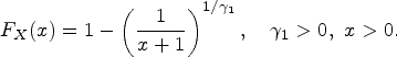
Within this subsection, based on Theorems 3.1 to 4.4, we analyze the asymptotic properties by considering some chosen copulas fulfilling Assumptions $S_{1}$ and $S_{2}$ . Thus, we focus on heavy-tailed distributions for the marginal distribution of $X$ and uniformly select the Pareto distribution for each case.

F_{X} (x) = 1 - {(\frac{1}{x + 1})}^{1 / γ_{1}}, γ_{1} > 0, x > 0.

We recall that the Pareto distribution is often used to model extreme events or phenomena with heavy tails, making it relevant in the context of extreme risk analysis.

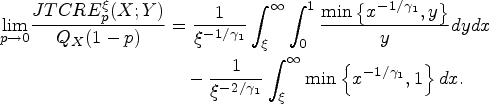
4.2.1. Independence Survival Copulas

The independence survival copulas is $\hat{C} (v, u) = v u$ ,

lim_{t \to 0} \frac{\hat{C} (t x, t y)}{t^{2}} = x y := ℓ (x, y) \equiv ℓ^{'} (x, y),

then the tail order

k = 2

. The applicability of Theorem 3.1 to this case is limited because it is not possible to satisfy both conditions,

1 + γ_{1} - k > 0

and

γ_{1} \in (0, 1),

simultaneously.

By Theorem 4.2 we have the following

lim_{p \to 0} \frac{J T C R E_{p} (X; Y)}{Q_{X} (1 - p)} = \int_{1}^{\infty} \int_{0}^{1} \frac{x^{- 1 / γ} y}{y} - \frac{x^{- 1 / γ} y}{y} d y d x = 0.

(24)

4.2.2. Fréchet–Hoeffding Upper Bound Survival Copula

The survival copulas of the form $\hat{C} (x, y) = min {x, y}$ are referred to as the Fréchet–Hoeffding upper bound survival copula, such that

lim_{t \to 0} \frac{\hat{C} (t x, t y)}{t} = min {x, y} := ℓ (x, y),

(25)

which satisfies

S_{2}

for

k = 1

. Thus, from Theorem 3.1,

lim_{p \to 0} \frac{T C R E (X; Y)}{Q_{1} (1 - p)} = \frac{1 + γ_{1}}{1 - γ_{1}} \int_{0}^{\infty} min {x, y} d x = \frac{1 + γ_{1}}{(1 - γ_{1})^{2}} .

(26)

and by Theorem 4.4 we have the following

\begin{aligned} lim_{p \to 0} \frac{J T C R E_{p}^{ξ} (X; Y)}{Q_{X} (1 - p)} & = \frac{1}{ξ^{- 1 / γ_{1}}} \int_{ξ}^{\infty} \int_{0}^{1} \frac{min {x^{- 1 / γ_{1}}, y}}{y} d y d x \\ - \frac{1}{ξ^{- 2 / γ_{1}}} \int_{ξ}^{\infty} min {x^{- 1 / γ_{1}}, 1} d x . \end{aligned}

4.2.3. Clayton Survival Copulas

The Clayton survival copula can be expressed in the following form, which is a special case of the Archimedean copula.

\hat{C} (x, y) = ϕ (ϕ^{- 1} (x) + ϕ^{- 1} (y)) .

(27)

If we take the generator function in our example to be

ϕ (x) = (1 + x)^{- 1}

, then we obtain

\hat{C} (x, y) = (x^{- 1} + y^{- 1} - 1)^{- 1}

, which satisfies assumption

S_{2}

with

k = 1

, thus by Theorem 3.1 we have

ℓ (x, y) = (x + y)^{- 1} \Rightarrow lim_{p \to 0} \frac{T C R E (X; Y)}{Q_{X} (1 - p)} = \frac{γ_{1}}{1 - γ_{1}} \int_{0}^{\infty} \frac{1}{x^{- 1 / γ_{1}} + 1} d x .

(28)

Also,

ℓ^{'} (x, y) = \frac{ℓ (x, y)}{ℓ (1, 1)} = 2 (1 / x + 1 / y)^{- 1} .

(29)

Then for

0 < ξ \leq 1

, Theorem 4.4 implies that

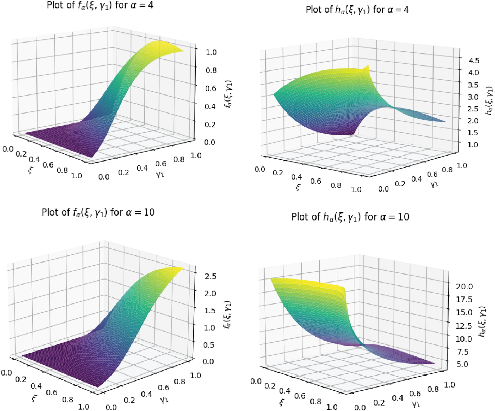
\begin{aligned} lim_{p \to 0} \frac{J T C R E_{p}^{ξ} (X; Y)}{Q_{X} (1 - p)} & = \frac{4}{ξ^{1 / γ_{1}} + 1} \int_{ξ}^{\infty} \int_{0}^{1} \frac{1}{y x^{1 / γ_{1}} + 1} d y d x \\ - \frac{8}{(ξ^{1 / γ_{1}} + 1)^{2}} \int_{ξ}^{\infty} \int_{0}^{1} \frac{1}{(x^{1 / γ_{1}} + 1) (y + 1)} d y d x . \end{aligned}

In order to investigate the influence of

ξ

and

γ_{1}

on the results established in Theorem 4.4, we graphically illustrate (in Figure 1) their effects by considering the Fréchet–Hoeffding upper bound survival copula and the Clayton survival copula. Formally, for all

α \in [0, \infty]

, we define the following functions

\begin{aligned} f_{α} (ξ, γ_{1}) & = \frac{1}{ξ^{- 1 / γ_{1}}} \int_{ξ}^{α} \int_{0}^{1} \frac{min {x^{- 1 / γ_{1}}, y}}{y} d y d x - \frac{1}{ξ^{- 2 / γ_{1}}} \int_{ξ}^{α} min {x^{- 1 / γ_{1}}, 1} d x, \end{aligned}

(30)

\begin{aligned} h_{α} (ξ, γ_{1}) & = \frac{1}{ξ^{- 1 / γ_{1}}} \int_{ξ}^{α} \int_{0}^{1} \frac{min {x^{- 1 / γ_{1}}, y}}{y} d y d x - \frac{1}{ξ^{- 2 / γ_{1}}} \int_{ξ}^{α} min {x^{- 1 / γ_{1}}, 1} d x . \end{aligned}

(31)

Figure 1.

Limit behaviors for the considered survival copulas.

It is straightforward to see that, for a bivariate continuous non-negative random vector $(X, Y)$ , $f_{α} (ξ, γ_{1})$ and $h_{α} (ξ, γ_{1})$ define a truncated version of $lim_{p \to 0} \frac{J T C R E_{p}^{ξ} (X; Y)}{Q_{X} (1 - p)}$ for the Fréchet–Hoeffding upper bound survival copula and Clayton survival copulas, respectively.

Remark 4

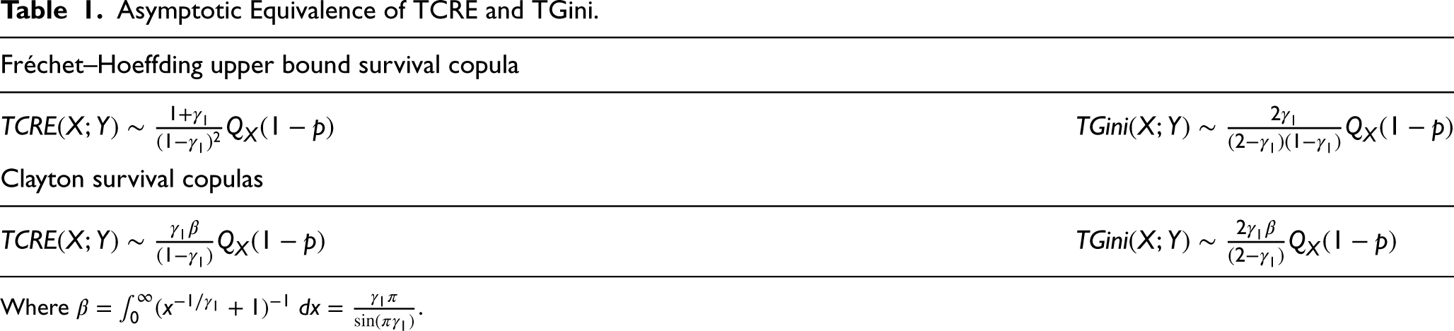
Based on our results and the findings of Sun and Chen (2022), Table 1 summarizes and compares the asymptotic equivalence for TCRE and TGini for the considered copulas.

Table 1.

Asymptotic Equivalence of TCRE and TGini.

Fréchet–Hoeffding upper bound survival copula
$T C R E (X; Y) \sim \frac{1 + γ_{1}}{(1 - γ_{1})^{2}} Q_{X} (1 - p)$	$T G i n i (X; Y) \sim \frac{2 γ_{1}}{(2 - γ_{1}) (1 - γ_{1})} Q_{X} (1 - p)$
Clayton survival copulas
$T C R E (X; Y) \sim \frac{γ_{1} β}{(1 - γ_{1})} Q_{X} (1 - p)$	$T G i n i (X; Y) \sim \frac{2 γ_{1} β}{(2 - γ_{1})} Q_{X} (1 - p)$

Where $β = \int_{0}^{\infty} (x^{- 1 / γ_{1}} + 1)^{- 1} d x = \frac{γ_{1} π}{\sin (π γ_{1})}$ .

5. From Theory to Practice

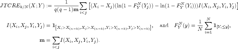
Let us consider an intermediate sequence $q$ obtained from a discrete random sample ${(X_{i}, Y_{i})}_{i = 1}^{N}$ . The sets of order statistics of ${X_{i}}_{i = 1}^{N}$ and ${Y_{i}}_{i = 1}^{N}$ are denoted by ${X_{(1)}, X_{(2)}, \dots, X_{(N)}}$ and ${Y_{(1)}, Y_{(2)}, \dots, Y_{(N)}}$ , respectively, such that ${X_{(1)} \leq X_{(2)} \leq \dots \leq X_{(N)}}$ and ${Y_{(1)} \leq Y_{(2)} \leq \dots \leq Y_{(N)}}$ . A non-parametric estimator version of JTCRE can be constructed for a specific chosen level of risk $p = q / N$ as follows:

\begin{aligned} J T C R E_{k / N} (X; Y) & := \frac{1}{q (q - 1) m} \sum_{i < j} [(X_{i} - X_{j}) (\ln (1 - F_{Y}^{N} (Y_{j})) - \ln (1 - F_{Y}^{N} (Y_{i}))) I (X_{i}, X_{j}, Y_{i}, Y_{j})] \\ I (X_{i}, X_{j}, Y_{i}, Y_{j}) & = 1_{[X_{i} > X_{(n - k)}, X_{j} > X_{(n - k)}, Y_{i} > Y_{(n - k)}, Y_{j} > Y_{(n - k)}]}, and F_{Y}^{N} (y) = \frac{1}{N} \sum_{i = 1}^{N} 1_{[Y_{i} \leq y]}, \\ m & = \sum_{i < j} I (X_{i}, X_{j}, Y_{i}, Y_{j}) . \end{aligned}

The non-parametric estimator for JTCRE is given analogously to the JTGini estimator presented in the concluding remarks of Sun and Chen (2022). A detailed analysis of this estimator will be presented in a forthcoming work, following the established approaches for TGini in Hou and Wang (2021) and TCRE in Sun et al. (2022).

To illustrate the real-world applicability of our proposed estimator, we implement it on a real-world dataset. The analysis focuses on six prominent companies listed on the American financial market: Chevron Corporation (CVX), Merck (MRK), Broadcom (AVGO), Adobe (ADBE), JPMorgan Chase (JPM), and Eli Lilly and Company (LLY). The SP 500 Index serves as the benchmark variable. Our analysis utilizes daily loss data for the aforementioned companies, spanning the period from January 1, 2015, to December 31, 2022. This timeframe notably encompasses the COVID-19 pandemic, a significant global extreme event that demonstrably impacted stock markets (see Ben Hssain et al., 2022).

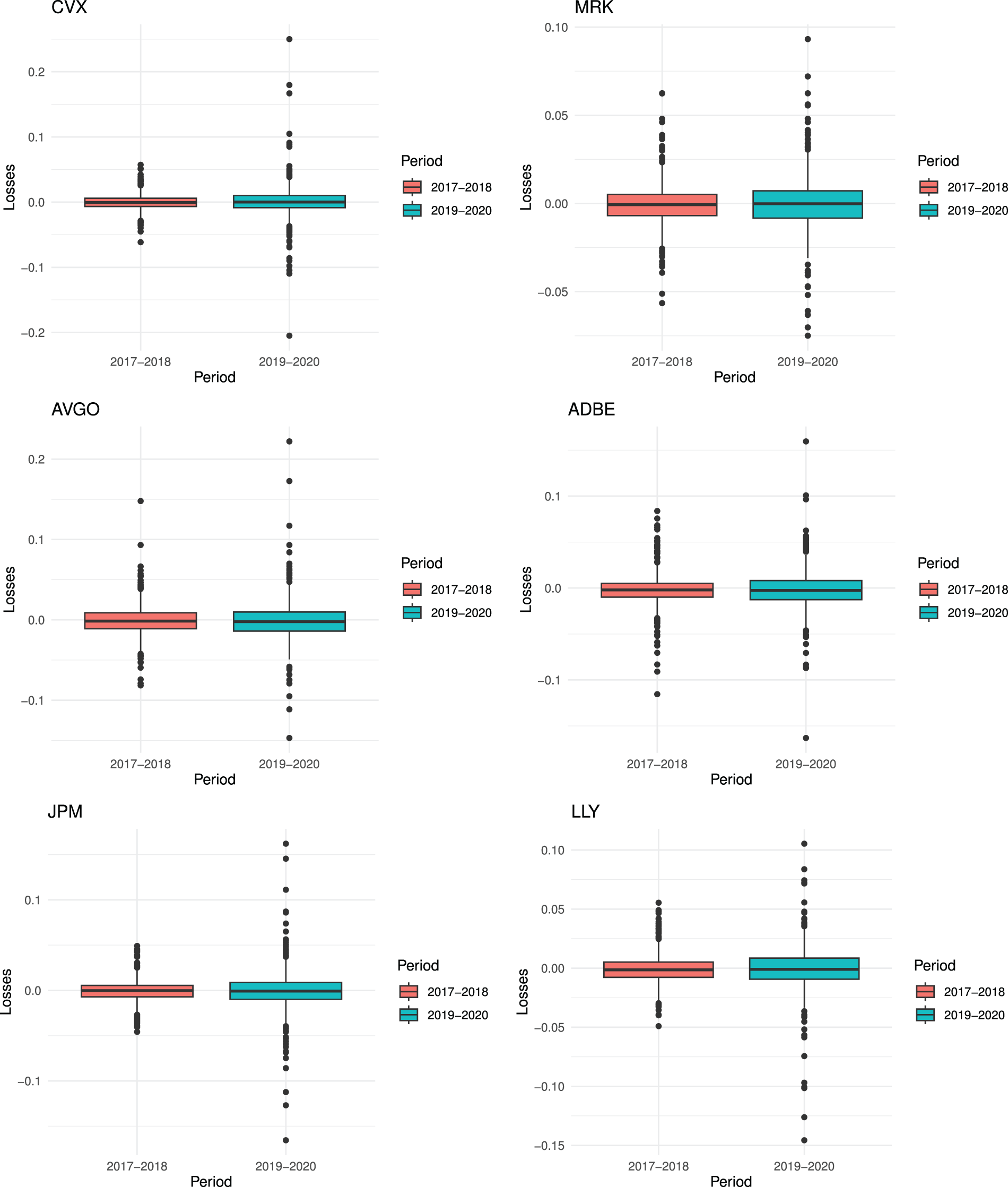
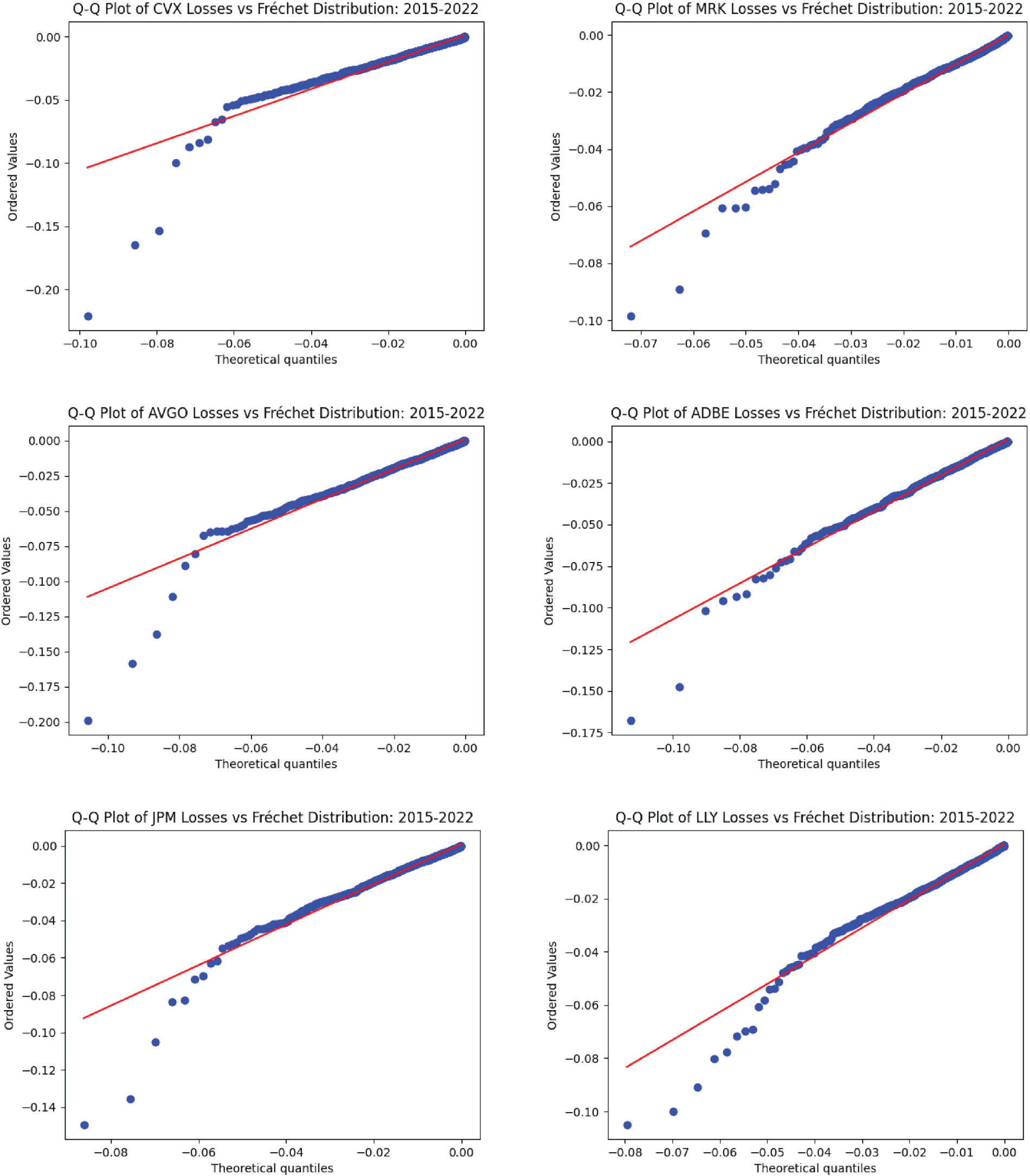
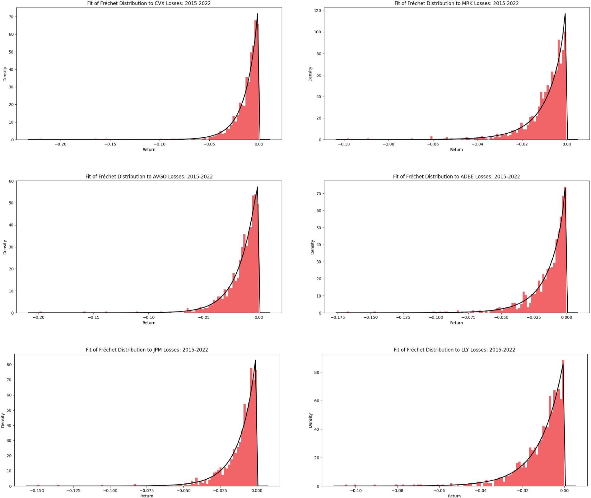
Firstly in Appendix B (Figure 2) we illustrate boxplots that visually represent the distribution of daily losses across the six companies. The data is segmented into two distinct periods: pre-COVID-19 (2017–2018) depicted by blue boxes, and during COVID-19 (2019–2020) shown by red boxes. A clear distinction is observable, with losses during the COVID-19 period exhibiting a significant increase compared to the pre-pandemic period. The economic disruption caused by the COVID-19 pandemic could potentially influence the behavior of financial returns, potentially increasing the likelihood of them falling within the Fréchet domain of attraction. To explore this further, comparisons with the Fréchet distribution are presented in Appendices (Figures 3 and 4).

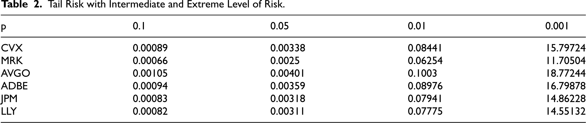
Secondly, in order to assess the impact of the entire market on each stock during a black represented by COVID-19, Table 2 summarizes the estimated JTCRE for various risk levels, specifically intermediate levels ( $p = 0.1$ or $0.05$ ) and extreme levels ( $p = 0.01$ or $0.001$ ). JTCRE values demonstrably increase as $p$ decreases, with the largest value observed at $p = 0.001$ . Notably, JTCRE remains constant for $p \leq 0.001$ . This behavior economically suggests the potential cost of the COVID-19, as measured by JTCRE. Consequently, JTCRE can be a valuable tool for setting thresholds in decision-making processes during extreme market scenarios.

Table 2.

Tail Risk with Intermediate and Extreme Level of Risk.

p	0.1	0.05	0.01	0.001
CVX	0.00089	0.00338	0.08441	15.79724
MRK	0.00066	0.0025	0.06254	11.70504
AVGO	0.00105	0.00401	0.1003	18.77244
ADBE	0.00094	0.00359	0.08976	16.79878
JPM	0.00083	0.00318	0.07941	14.86228
LLY	0.00082	0.00311	0.07775	14.55132

Conclusion

This paper underscores the imperative of accounting for exceptional events that can diverge from normalcy, such as crisis periods. Through a comprehensive analysis, we have delved into the asymptotic behaviors of Tail-based Cumulative Residual Entropy (TCRE), Joint TCRE, and its proposed generalized version by considering various hypotheses and encompassing both tail-dependent and tail-independent scenarios, which are modeled by copula properties. Furthermore, examples based on classical copulas and a real data application are provided. Thus, this paper advances our comprehension of extreme risk by shedding light on rare events and tail behaviors. Through the lens of the proposed measures, we are equipped to evaluate and manage risk in the ever-changing landscape of financial markets.

This study paves the way for future research endeavors, such as exploring more statistical characteristics, including asymptotic properties and convergence, of the proposed estimator of JTCRE and encouraging its application.

Footnotes

Funding

The author(s) disclosed receipt of the following financial support for the research, authorship, and/or publication of this article.

Declaration of Conflicting Interests

The author(s) declared no potential conflicts of interest with respect to the research, authorship and/or publication of this article.

Appendix A

As in Sun et al. (2022), lest us define $h (x, ε) := 2 x^{1 - ε}$ for $0 < x < 1$ and $0 < ε < 1 - γ_{1}$ . Then by Proposition B.1.9 in Haan & Ferreira (2006) there exist a constant $p_{0} \in (0, 1)$ , such that for all $0 < p < p_{0}$ , $s_{p} (x, ε) \leq h (x, ε)$ . It is evident that (32)

\int_{0}^{\infty} s_{p} (x) \land 1 d x^{- γ_{1}} \leq \int_{0}^{\infty} d x^{- γ_{1}} + \int_{0}^{1} h (x, ε) d x^{- γ_{1}} < \infty .

Assume that

b \in (0, 1)

satisfied

h (b, ε) = 1

. Then

\begin{aligned} \int_{0}^{\infty} \int_{0}^{1} (\frac{s_{p} (x)}{y} \land 1) d y d x^{- γ_{1}} & \leq \int_{0}^{1} \int_{0}^{1} (\frac{h (x, ε)}{y} \land 1) d y d x^{- γ_{1}} + \int_{1}^{\infty} d x^{- γ_{1}} \\ = \int_{b}^{1} d x^{- γ_{1}} + \int_{0}^{b} (\int_{0}^{h (x, ε)} d y + \int_{h (x, ε)}^{1} \frac{h (x, ε)}{y} d y) d x^{- γ_{1}} + \int_{1}^{\infty} d x^{- γ_{1}} \\ = \int_{b}^{1} d x^{- γ_{1}} + \int_{0}^{b} h (x, ε) d x^{- γ_{1}} + \int_{0}^{b} \int_{h (x, ε)}^{1} \frac{h (x, ε)}{y} d y d x^{- γ_{1}} + \int_{1}^{\infty} d x^{- γ_{1}} . \end{aligned}

It is obvious that

\int_{b}^{1} d x^{- γ_{1}} < \infty

\int_{1}^{\infty} d x^{- γ_{1}} < \infty

, and

\int_{0}^{b} h (x, ε) d x^{- γ_{1}} < \infty .

Furthermore,

\begin{aligned} \int_{0}^{b} \int_{h (x, ϵ)}^{1} \frac{h (x, ε)}{y} d y d x^{- γ_{1}} & = - \int_{0}^{b} h (x, ε) \ln g (x, ε) d x^{- γ_{1}} = - \int_{0}^{b} 2 x^{1 - ε} \ln (2 x^{1 - ε}) (- γ_{1}) x^{- (γ_{1} + 1)} d x \\ = \int_{0}^{1 / 2} 2 x \ln 2 x \frac{γ_{1}}{1 - ε} x^{\frac{ε - (γ_{1} + 1)}{1 - ϵ}} d x \\ \leq \int_{0}^{1 / 2} 2 x (2 x - 1) \frac{γ_{1}}{1 - ε} x^{\frac{ε - (γ_{1} + 1)}{1 - ϵ}} \\ = \int_{0}^{1 / 2} \frac{4 γ_{1}}{1 - ε} x^{\frac{ε - (γ_{1} + 1)}{1 - ϵ}} d x - \int_{0}^{1 / 2} \frac{2 γ_{1}}{1 - ε} x^{\frac{- γ_{1}}{1 - ε}} < \infty, \end{aligned}

which implies that (33)

\int_{0}^{\infty} \int_{0}^{1} (\frac{s_{p} (x)}{y} \land 1) d y d x^{- γ_{1}} < \infty .

Appendix B: Boxplots of Losses

Figure 2.

Boxplots of losses.

Appendix C: QQ Plot of Losses

Figure 3.

QQ plot of losses vs Frechet distribution.

Appendix D: Fit of Frechet Distribution

Figure 4.

Fit of Frechet distribution.

References

Acerbi

. (2002). Spectral measures of risk: A coherent representation of subjective risk aversion. Journal of Banking & Finance, 26(7), 1505–1518. https://doi.org/10.1016/S0378-4266(02)00281-9

Acharya

V. V.

Pedersen

L. H.

Philippon

Richardson

. (2017). Measuring systemic risk. The Review of Financial Studies, 30(1), 2–47. https://doi.org/10.1093/rfs/hhw088

Artzner

Delbaen

Eber

J. M.

Heath

(1999). Coherent measures of risk. Mathematical Finance, 9(3), 203–228. https://doi.org/10.1111/1467-9965.00068

Asimit

A. V.

. (2018). Measuring the tail risk: An asymptotic approach. Journal of Mathematical Analysis and Applications, 463(1), 176–197. https://doi.org/10.1016/j.jmaa.2018.03.019

Ben Hssain

Agouram

Lakhnati

(2022). Impact of COVID-19 pandemic on Moroccan sectoral stocks indices. Scientific African, 17, e01321. https://doi.org/10.1016/j.sciaf.2022.e01321

Ben Hssain

Berkhouch

Lakhnati

(2024). Portfolio selection based on extended Gini shortfall risk measures. Statistics & Risk Modeling, 41(1-2), 27–48. https://doi.org/10.1515/strm-2023-0001

Berkhouch

Lakhnati

Righi

M. B.

(2018). Extended Gini-type measures of risk and variability. Applied Mathematical Finance, 25(3), 295–314. https://doi.org/10.1080/1350486X.2018.1538806

Bingham

N. H.

Goldie

C. M.

Teugels

J. L.

(1989). Regular Variation (No. 27). Cambridge university press.

Broda

S. A.

Krause

Paolella

M. S.

(2018). Approximating expected shortfall for heavy-tailed distributions. Econometrics and Statistics, 8, 184–203. https://doi.org/10.1016/j.ecosta.2017.07.003

10.

Cai

J. J.

Einmahl

J. H.

Haan

Zhou

(2015). Estimation of the marginal expected shortfall: The mean when a related variable is extreme. Journal of the Royal Statistical Society Series B: Statistical Methodology, 77(2), 417–442. https://doi.org/10.1111/rssb.12069

11.

Chen

C. W. S.

Watanabe

Lin

E. M. H.

(2023). Bayesian estimation of realized GARCH-type models with application to financial tail risk management. Econometrics and Statistics, 28, 30–46. https://doi.org/10.1016/j.ecosta.2021.03.006

12.

Das

Fasen-Hartmann

(2018). Risk contagion under regular variation and asymptotic tail independence. Journal of Multivariate Analysis, 165, 194–215. https://doi.org/10.1016/j.jmva.2017.12.004

13.

El Qalli

Said

(2023). Some systemic risk indicators. Risk and Decision Analysis, 9(2-4), 39–56. https://doi.org/10.3233/RDA-231521

14.

Furman

Wang

Zitikis

. (2017). Gini-type measures of risk and variability: Gini shortfall, capital allocations, and heavy-tailed risks. Journal of Banking & Finance, 83, 70–84. https://doi.org/10.1016/j.jbankfin.2017.06.013

15.

Gardes

(2022). On tail-risk measures for non-integrable heavy-tailed random variables. Econometrics and Statistics. https://doi.org/10.1016/j.ecosta.2022.10.003

16.

Haan

Ferreira

(2006). Extreme Value Theory: An Introduction. Springer. https://doi.org/10.1007/0-387-34471-3

17.

Hou

Wang

(2019). Nonparametric inference for distortion risk measures on tail regions. Insurance: Mathematics and Economics, 89, 92–110. https://doi.org/10.1016/j.insmatheco.2019.09.003

18.

Hou

Wang

(2021). Extreme and inference for tail Gini functionals with applications in tail risk measurement. Journal of the American Statistical Association, 116(535), 1428–1443. https://doi.org/10.1080/01621459.2020.1730855

19.

Chen

(2020). On a family of coherent measures of variability. Insurance: Mathematics and Economics, 95, 173–182. https://doi.org/10.1016/j.insmatheco.2020.10.005

20.

Hua

Joe

(2011). Tail order and intermediate tail dependence of multivariate copulas. Journal of Multivariate Analysis, 102(10), 1454–1471. https://doi.org/10.1016/j.jmva.2011.05.011

21.

Tan

K. S.

Yang

(2021). Tail dependence and heavy tailedness in extreme risks. Insurance: Mathematics and Economics, 99, 282–293. https://doi.org/10.1016/j.insmatheco.2021.03.016

22.

Ledford

A. W.

Tawn

J. A.

(1996). Statistics for near independence in multivariate extreme values. Biometrika, 83(1), 169–187. https://doi.org/10.1093/biomet/83.1.169

23.

(2013). Stochastic Orders in Reliability and Risk Honor of Professor Moshe Shaked. Springer. https://link-springer-com-443.web.bisu.edu.cn/content/pdf/10.1007/978-1-4614-6892-9.pdf

24.

Nelsen

R. B.

(2006). An Introduction to Copulas. Springer science & business media. https://doi.org/10.1007/0-387-28678-0

25.

Rao

Chen

Vemuri

B. C.

Wang

(2004). Cumulative residual entropy: A new measure of information. IEEE Transactions on Information Theory, 50(6), 1220–1228. https://doi.org/10.1109/TIT.2004.828057

26.

Sklar

(1959). Fonctions de repartition an dimensions et leurs marges. Publ inst statist univ Paris, 8, 229–231.

27.

Sun

Chen

(2022). Extreme behaviors of the tail Gini-type variability measures. Probability in the Engineering and Informational Sciences, 37(4), 928–942. https://doi.org/10.1017/S0269964822000304

28.

Sun

Chen

(2022). Statistical inference for tail-based cumulative residual entropy. Insurance: Mathematics and Economics, 103, 66–95. https://doi.org/10.1016/j.insmatheco.2022.01.002

29.

Zuo

Yin

(2023). Covariance representations and coherent measures for some entropies. Entropy, 25(11), 1525. https://doi.org/10.3390/e25111525