Confidence Intervals for the Model Performance Metrics Under the Imbalanced Classification: Evaluating SMOTE’s Impact on Metrics’ Reliability

Abstract

AI applications in finance including those for the probability of default modeling largely involve using ML classification tools. Oversampling the very minor (very underrepresented) class of defaulted borrowers seems to be a must-be-done step always. However, by crunching more than a thousand of confidence intervals for the classification accuracy metrics, we demonstrate when such oversampling is worth engaging in. Moreover, we argue to what portion of total initial sample size such oversampling should be carried out. Our findings are valuable primarily for the credit risk modeling and Internal Ratings Based (IRB) banks, but are not limited to those and have general applications for the binary classifications in ML domain.

Keywords

credit risk precision recall F1 classification clustering segmentation IRB

I prefer true but imperfect knowledge,

even if it leaves much indetermined and unpredictable,

to a pretence of exact knowledge that is likely to be false.

Hayek (1974),

Nobel Prize lecture

1. Introduction

The Basel Committee report BCBS (2017) might be named the first formal recognition of the material artificial intelligence (AI) proliferation in the finance domain. Formally, it even led to the introduction of the new terms like FinTech, RegTech, and SupTech. At the time the committee saw only technological risks posed by the proliferation of AI, machine learning (ML), and advanced data analytics considered jointly. As a result, the committee recommended strengthening the information technologies (IT) with which the bank is equipped, see BCBS (2017, pp. 28).

Since then the AI/ML use made that significant progress that the associated risks stopped being limited solely by IT ones. More conceptual issues arose. Those include the ethical ones whether an algorithm should be allowed or not to discriminate one cohort of customers to the detriment (rarely - to the benefit) of another. This led to the discussion of the ethical probability of default (PD) models in papers like Fuster et al. (2018) and Szepannek and Luebke (2021). The European Parliament extended the discussion by making an unprecedented step and publishing a pan-European AI regulation act, see Europarliament (2023).

So far, it seems that methodologically everything is clear with the development of AI in finance, and it is only the issue of the available (sufficient) computational capacities based on graphical processing unit (GPU). Such thoughts gave rise to the terms of GPU-rich and GPU-poor companies distinguishing companies which have enough access to the needed GPU capacities and those which do not have, see The Economist (2024).

However, today seems to be right the time when we may fall into the fundamental trap created by our obsession with the exact prediction and hence recommendation skills of AI modules driven by the underlying ML solutions. The nature of the trap is as follows. The recent ML trend allows software to elaborate own programming codes and models, in particular (though still far from ideally targeted ones as developed by experienced coders). The AI solution of interest is likely to continue reprogramming the specific model as far as its output performance (accuracy) metrics outpaces that of the previous one. Such a process goes on as in most cases it is the point estimates of the performance metrics which rise, though sometimes at a tiny growth rate. From the outside perspective such an improvement process in addition vastly consumes GPU power making any company GPU-poor in essence.

Nevertheless, the improvement process is not as endless as it seems and as it was in the legend when Achilles failed to outrun the turtle. As a reminder, the legend says that the mighty Achilles is unable to reach the turtle, because every time when he reaches it, the turtle is able to move some distance away. Though the distance might be small, but it is still there and Achilles cannot reach the turtle never.

For a detailed mathematical explanation of this paradox and its original interpretation, please refer to the Feng (2023). In fact, most models become similar when the model performance metrics reach a particular threshold for a combination of classes and features. Such similarity is well captured by the confidence intervals (CI) for the performance metrics, which unfortunately are not that wide-spread though well-known in probability theory. Hence, if the AI algorithm for a credit scoring or fraud detection in finance reached the stage when the upper boundary of the accuracy metrics CI is almost equal to one (to 100%), it is clear that any novel model cannot discriminate poor borrowers from good ones any better (unless there happens a region-wide shock and overall model prediction quality deteriorates). This could mean that AI software may get rise in efficiency by not crunching the code and numbers any longer and by economizing the GPU capacity for other tasks.

The use of confidence intervals for the performance metrics of ML models in finance is not novel. Moreover, the cases when one of the two classes is materially underrepresented is also known (consider the term low-default portfolio (LDP), for instance). Oversampling minor class is a typical industry solution. However, no one, to the best of our knowledge, studied the evolution of confidence intervals for the performance metrics of the models in finance when such oversampling is undertaken. We intend to close this gap by using a “black box ”approach (we use such a term as we rely upon the existing library (black box) to oversample data).

As a preview of our findings, we show that excessive oversampling (at the extreme when equalizing the proportions of the minor and major classes) leads to the rise in the width of the confidence intervals of the performance metrics making models more indistinguishable from each other, and by overall sacrificing the model performance quality. The practical implication from here is to oversample at a limited degree. Then and only then the model developer (or AI software supposedly in the near future) may be able to evidence the true improvement in the model performance.

To explain how we arrive at our findings, we start with the literature review in Section 2. We describe the methodology in Section 3. The findings follow in Section 4. We conclude in Section 5.

2. Literature Review

AI applications in finance, though numerous, can be broadly grouped into several groups of which classification tasks continue occupying important place. Those tasks might include distinguishing good and bad borrowers, clients prone to churn and not, online users willing to choose a product or not, fraudsters and general users. Solving classification (properly discriminating) in-between these two groups forms the basis for further recommendation system development.

Hence, it is vitally important to be efficient in solving classification tasks when applying AI and ML in finance. Seems lots has been discussed about it in Mirkin (2016) and Raschka and Mirjalili (2019), for instance. However, gaps still exist. Those relate to situations when one of two classes is materially underrepresented (such a class might be called a very minor one, while the residual class is a major one). A fast, but not always worthy typical solution is to oversample. This is why we intend to study consequences of such a step given often omitted specifics for the confidence intervals when applied to the classification accuracy metrics.

To do so, we first discuss the papers when dealing with minor classes are not a one-off case. Namely, it is the domain of probability of default (PD) modeling and developing PD models for banks specifically. Nevertheless, the findings are of value to other areas, including inter alia cyberfraud detection. Second, we remind approaches to handling a minor class when it might be assumed to be underrepresented in a non-systematic manner. This is where the suggestion to oversample the minor class is being born. Third, we focus on how to choose the best classification model as it is exactly the criteria intended to be improved when oversampling. Fourth, we rehearse the importance of monitoring the confidence intervals for the classification metrics, not limited to their mean values.

2.1. PD Modeling

The first formal probability of default (PD) models were proposed in the papers by Beaver (1966), Altman (1968) and Ohlson (1980). Authors of these papers used a countable number of observations driven by the computational capabilities of the first computers. These often equaled a couple of dozen company-year (or just company) observations. Moreover, the samples of defaulted and non-defaulted companies typically equaled in size, giving no rise to the issue of handing a minor class.

Since then software and financial services industries evolved that much that PD models started being considered as part of the financial regulation. Formally, the Basel Committee on Banking Supervision (BCBS) allowed them as a part of the Basel II Internal Ratings-Based (IRB) approach, see BCBS (2006). Prior to formal adoption, the committee published a comprehensive survey of progress in classification models development, and more specifically to that of PD models in BCBS (2000). It was highly likely that the PD model conceptual approval by the international financial regulation standards setter of BCBS triggered the research boom in the area.

As a result, we come across the use of conventional econometric and multivariate statistical analysis tools to develop PD models as discussed by Kumar and Ravi (2007) and Altman (2018). Same time the use of ML tools gains its popularity as can be seen from the following non-exhausting list of papers: Chen et al. (2006), Fantazzini and Figini (2009), Korol and Korodi (2010), Tinoco and Wilson (2014), Geng et al. (2015), Jabeur and Fahmi (2018), Shibitov and Mamedli (2019), Qu et al. (2019), Dendramis et al. (2020), Kim et al. (2020), Moscatelli et al. (2020), Kim et al. (2021), Faraj et al. (2021), Pang et al. (2021), Merćep et al. (2021) and Liu et al. (2022).

PD models were developed for many localities. To name a few, Jabeur and Fahmi (2018) considered France, Chen et al. (2006) and Liu et al. (2022) - China, Altman et al. (2008) - the UK, Tian and Yu (2017) - Japan, Bisogno et al. (2018) - the EU, Kristóf and Virág (2020) - Hungary, Merćep et al. (2021) - Croatia.

Most academic papers present PD models for the retail borrowers because the segment is typically characterized by the enormous number of observations and defaults. PD models for corporate borrowers appear less often, while banks are the rarest research objects. For instance, they are handled in the following relevant works: Bräuning et al. (2020) and Durand et al. (2021) for the EU, Yuksel et al. (2015) for Turkey, Shrivastava et al. (2020) for India, Kočenda and Iwasaki (2022) for Japan, Kocagil et al. (2002), Moody’s Analytics (2016) and Cole et al. (2020) for the USA, Obeid (2021) for the Persian Gulf countries, and Cheong and Ramasamy (2019); Kristóf (2021) for others. Relevant reviews are available at Kumar and Ravi (2007) and Citterio (2020).

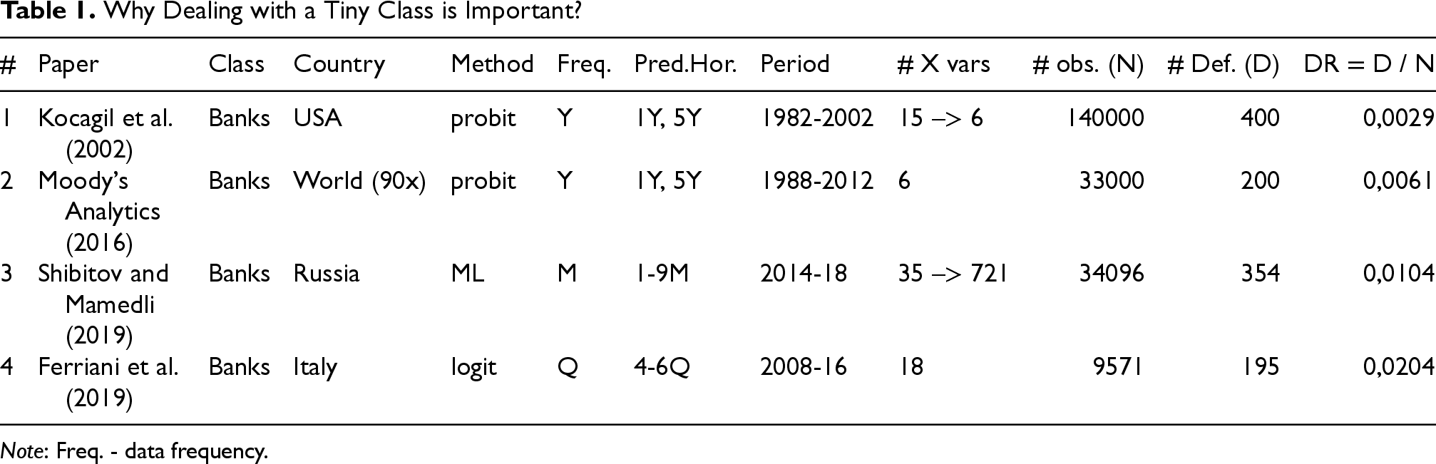
The reason for such rarity of the PD model for banks can be vividly seen from the illustrative Table 1. Nowadays, as well as 20 years ago, financial institutions (FI) tend mostly not to default. The proportion of defaulted cases at maximum approaches 2% of the total sample, being as small as less than half of the percentage point (see last column of Table 1). This is why financiers tend to call the FI segment a low default portfolio (LDP). AI/ML practitioners eagerly see the problem (defaulted) cases in the segment as the very minor class with the non-defaulters being a very major one. Despite the widespread regulatory doctrine of “too big to fail,” systemic collapses of major financial institutions still occur, as exemplified by the historical crises of Credit Suisse. The 2008 failure of Lehman Brothers and near-collapses of other large firms critically deepened the recession by destabilizing markets, freezing credit flows, collapsing asset values, and eroding public trust, whereas smaller firm failures have not meaningfully threatened the global financial system’s stability (see Johnson and Mamun (2012)).

Table 1.
Why Dealing with a Tiny Class is Important?

# Paper Class Country Method Freq. Pred.Hor. Period # X vars # obs. (N) # Def. (D) DR = D / N

1 Kocagil et al. (2002) Banks USA probit Y 1Y, 5Y 1982-2002 15 –> 6 140000 400 0,0029

2 Moody’s Analytics (2016) Banks World (90x) probit Y 1Y, 5Y 1988-2012 6 33000 200 0,0061

3 Shibitov and Mamedli (2019) Banks Russia ML M 1-9M 2014-18 35 –> 721 34096 354 0,0104

4 Ferriani et al. (2019) Banks Italy logit Q 4-6Q 2008-16 18 9571 195 0,0204

#	Paper	Class	Country	Method	Freq.	Pred.Hor.	Period	# X vars	# obs. (N)	# Def. (D)	DR = D / N
1	Kocagil et al. (2002)	Banks	USA	probit	Y	1Y, 5Y	1982-2002	15 –> 6	140000	400	0,0029
2	Moody’s Analytics (2016)	Banks	World (90x)	probit	Y	1Y, 5Y	1988-2012	6	33000	200	0,0061
3	Shibitov and Mamedli (2019)	Banks	Russia	ML	M	1-9M	2014-18	35 –> 721	34096	354	0,0104
4	Ferriani et al. (2019)	Banks	Italy	logit	Q	4-6Q	2008-16	18	9571	195	0,0204

Note: Freq. - data frequency.

The collapse of Lehman Brothers and other major financial institutions severely exacerbated the crisis and recession by disrupting markets, hindering credit availability, triggering steep asset price declines, and undermining confidence. While the failures of smaller, less interconnected firms remain concerning, they have not meaningfully threatened the broader stability of the financial system.

2.2. Missing Data and Oversampling

Though the FI segment is not rich in defaults, the financiers solicited PD models for the segment. There are several solutions on how to act, according to Raschka and Mirjalili (2019, pp. 267–270):

to oversample the minor class, Liu (2021); Nunes et al. (2021);

to undersample the major class.

to input missings, Audigier et al. (2021);

Koziarski (2021) opts for a combination of over- and undersampling. However, oversampling is grounded on the strong assumptions. According to Rubin (1976) classification, it is assumed that the data (default cases) is missing either completely at random (MCAR), or just at random (MAR). However, Carreras et al. (2021) argues that if the data is of MCAR type, then oversampling is not needed, as one is to add pure noise not-impacting the model of interest.

On the contrary, the possibility of data being missing not at random (MNAR) is rarely checked. To be fair, in the absence of extra defaults, the feasibility of such verification by itself is under question. Pereira et al. (2019) offers arguments to ignore MNAR, as it stems from situations when the data was not collected or was wrongly collected via a survey. Financial default data has a more regular nature, and only extreme force-major events might trigger systematic unaccounting of many default cases. Alternatively, when wishing to handle MNAR cases, one may drift towards Heymans and Twisk (2022) who suggests modeling the missing data. But to do so, one should properly study such MNAR cases, then calibrate the data generating process parameters. One can do the latter step only by using the available limited (LDP) cases. Hence, we also neglect the possibility of MNAR observations here.

2.3. Classification Accuracy (Model Performance) Metrics

ML practitioners tend to oversample minor class as rule of thumb. Our objective here is to demonstrate cases when such oversampling is worth undertaking and when it is not. To answer this question, we should first inquire what objective is targeted when oversampling. The ML practitioners seek to improve (increase) the model quality (its performance metrics), i.e., the model developers wish the model to better discriminate (segment, classify, cluster) the incoming data into two classes (in case of PD model into defaulters and non-defaulters). The industry-standard is to look at precision, recall, accuracy and F1 indicators. The respective formulas are available in eqs. (1)–(4).

P r e c i s i o n = \frac{T P}{T P + F P},

(1)

where TP, FP are illustrated in Table 2.

R e c a l l = \frac{T P}{T P + F N},

(2)

where FN is presented in Table 2.

A c c u r a c y = \frac{A U R O C f o r t h e d e v e l o p e d m o d e l}{A U R O C f o r t h e p e r f e c t m o d e l},

(3)

where the numerator and denominator are computed after deducting the common surface (triangle) under the bisector line. We may recommend Engelmann et al. (2003) as one of the earlier papers in the finance domain for more details on AUROC use for the PD modeling.

F_{1} = \frac{2 \cdot P r e c i s i o n \cdot R e c a l l}{P r e c i s i o n + R e c a l l} = \frac{2}{(1 / R e c a l l) + (1 / P r e c i s i o n)} .

(4)

Table 2.

Stylized Default (Success) Prediction Matrix to Analyze Model Accuracy.

	Actual
Predicted	S (D)	F (ND)	Total
S (D)	True positives (TP)	False positives (FP)	$\cdot$ P
F (ND)	False negatives (FN)	True negatives (TN)	$\cdot$ N
Total			n

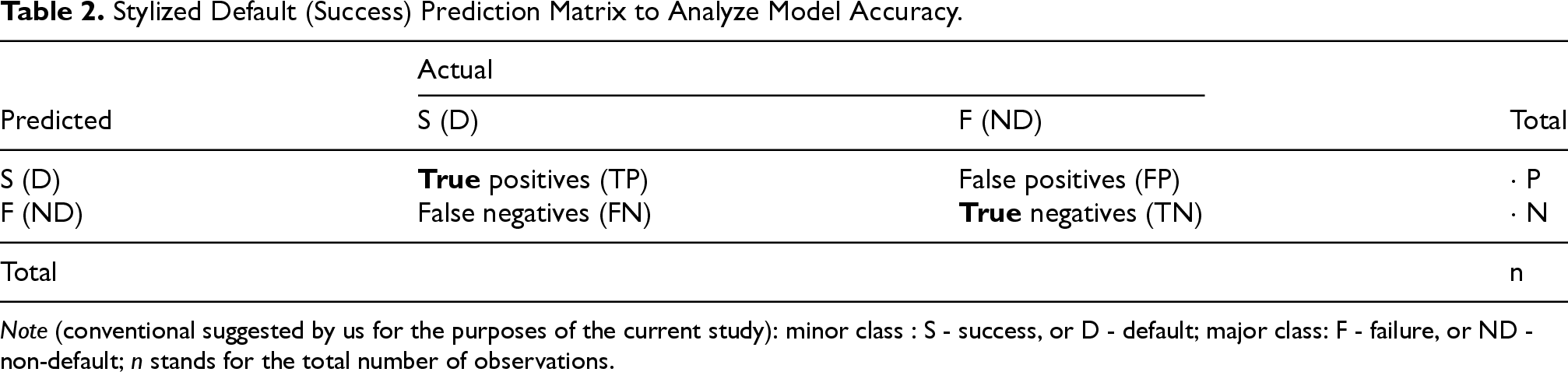
Note (conventional suggested by us for the purposes of the current study): minor class : S - success, or D - default; major class: F - failure, or ND - non-default; $n$ stands for the total number of observations.

2.4. Confidence Intervals for Proportions

We have evidenced above that PD models are well-studied, accuracy metrics are also commonly known. However, the problem - inter alia with the growing number of papers published and offering the better discriminating PD models - is that authors get obsessed with the improvement solely based on the mean values (point estimates) of the classification metrics of interest, e.g., Faraj et al. (2021, p. 24, Tab. 2), Kim et al. (2021, p. 170, Tab. 4), Pang et al. (2021, p. 10), Merćep et al. (2021, p. 10, Table 1 – p. 12, Table 6), Song et al. (2021, p.1489, Table 1), Liu et al. (2022, p. 10, Tab. 8).

Nevertheless, we should not forget that the performance metrics combine the number of realisations of a random variable, (often a dummy flag taking one in case of default and zero otherwise). They differ from each other in a way of such combination. Disregarding the mode of combination, the accuracy metrics by construction are still random variables in themselves. It means that the mere dominance (excess in arithmetic terms) of one point estimate over another may correspond to probabilistically equal values. To correctly judge upon the superiority of a particular model, when comparing PD models, one has to look at the confidence intervals of performance metrics, not limited to their point estimates. Moreover, as every accuracy metric is a proportion by construction ranging from zero to one, one should specifically look at the confidence intervals for (binomial) proportions.

The development of the confidence intervals (CIs) for proportions has passed through the following stages:

Wald CI, or normal approximation, see formula (5);

C I^{N} = (S / n) + / - γ_{α / 2} \cdot \sqrt{\frac{(S / n) \cdot [1 - (S / n)]}{n}},

(5)

where

γ_{α / 2} = N^{- 1} (α / 2)

is the quantile of the Normal (Gaussian) distribution at the

α / 2

significance level,

n

is the total number of observations,

S

is the number of successes (

F

is the number of failures, so that

n = S + F

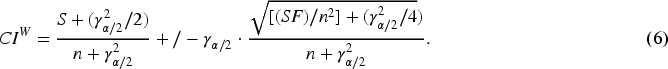
Wilson CI, see formulas (6)

C I^{W} = \frac{S + (γ_{α / 2}^{2} / 2)}{n + γ_{α / 2}^{2}} + / - γ_{α / 2} \cdot \frac{\sqrt{[(S F) / n^{2}] + (γ_{α / 2}^{2} / 4})}{n + γ_{α / 2}^{2}} .

(6)

where

γ_{α / 2} = λ = 2

is recommended in most cases, see Wilson (1927, p. 212).

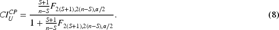
Clopper-Pearson (beta) CI, see Dunnigan (2008, p. 3), formulas (7), (8);

C I_{L}^{C P} = \frac{1}{1 + \frac{n - S + 1}{S} \cdot F_{2 (n - S + 1), 2 S, α / 2}},

(7)

where

F_{u, v, γ}

is the F-distribution with

(u, v)

degrees of freedom valued at

γ

significance level.

C I_{U}^{C P} = \frac{\frac{S + 1}{n - S} F_{2 (S + 1), 2 (n - S), α / 2}}{1 + \frac{S + 1}{n - S} F_{2 (S + 1), 2 (n - S), α / 2}} .

(8)

Orawo (2021) notes that Clopper-Pearson CI is more conservative, but wider than it is sufficient.

Agresti-Coull (AC) CI from Agresti and Coull (1998, p. 120), see formula (9);

C I^{A C} = \frac{S + (γ_{α / 2}^{2} / 2)}{n + γ_{α / 2}^{2}} + / - γ_{α / 2} \cdot \frac{\sqrt{(S F) \cdot [1 + (γ_{α / 2}^{2} / 2)] + (γ_{α / 2}^{4} / 4)}}{n + γ_{α / 2}^{2}} .

(9)

Jeffreys CI, see formulas (10), (11);

\begin{aligned} C I_{L}^{J} = B e t a (α / 2; S + 1 / 2, n - S + 1 / 2), \end{aligned}

(10)

\begin{aligned} C I_{U}^{J} = B e t a (1 - α / 2; S + 1 / 2, n - S + 1 / 2), \end{aligned}

(11)

where

B e t a (α, a_{1}, a_{2})

is the

α

-quantile of the Beta distribution with parameters

a_{1}

and

a_{2}

, see Brown et al. (2001, p. 108, eq. (7), (8));

L

and

U

indicate lower and upper boundaries of the confidence interval.

Brown et al. (2001) above all recommend using Jeffreys interval instead of normal approximation, as well as instead of Wilson’s and Agresti-Coull’s ones.

It is worth mentioning that Brown et al. (2001) refer to other types of confidence intervals such as the modified Wilson interval, modified Jeffreys interval, arcsine interval, logit interval, Bayesian interval, and likelihood ratio interval. These confidence intervals were not considered in the present study. The selection of the specific metrics used here is justified by their prevalence in the literature and based on the recommendations provided by the authors themselves in the conclusion of their work.

Hanson and Schuermann (2006) also examined the comparison of confidence intervals for default probability estimates using analytical methods, as well as parametric and nonparametric bootstrap approaches. The key distinction of our study lies in the fact that we analyze confidence intervals not for the default rates in the sample (see Table 2 in the appendix of Hanson and Schuermann (2006)), nor for the default probability (PD) distribution of a classification algorithm, but rather for the performance metrics of a binary classification algorithm. In fact, there is definitely a link between the confidence interval on the model performance metrics and the confidence interval on the model output. Hanson and Schuermann (2006) focused on the latter, we did it for the former, tracing a linkage between the two falls out of our research scope.

3. Simulation Experiment Design

3.1. Concept

We wish to study how confidence intervals for the classification accuracy metrics evolve under various scenarios. We look at three starting values of the minor class (e.g., default rates, DR): 0.1%, 3.0%, 10.0% of the total number of observations. These portions are the starting (baseline) values. We oversample them to reach up to 50% of the initial number of observations. For instance, take a $D R = 0.001$ (0.1%). The total number of observations is 20k; it yields us with 20 default cases and 19,080 non-default ones. When oversampling to 50% of the initial set, we get 10k defaults instead of just 20 ones. Hence, the new sample size is 10k + 19080 = 39080 observations. As for the DR=0.1% we run extra oversampling iterations to 10, 20, 30, 40% to be able to identify the threshold at which the CI width starts changing.

We use ten core features (independent factors) to delineate minor class observations from the major ones. We consider four possible factor combinations. Initially, a dataset with 10 core features was generated, where each feature contributes to forming the class label, this is the first dataset. Next, 5 independent columns were added to the original dataset; since these columns do not influence the class label, they are considered redundant, this is the second dataset. Next, 5 significant core features were removed from the original 10-core dataset, this is the third dataset. Finally, 5 redundant features were added to the 5-core dataset, yielding the fourth dataset.

For each model we evaluate four classification metrics as presented in subsection 2.3. For each of the metrics we present five confidence intervals (CIs) discussed in subsection 2.4. Hence, we derive five CI widths as differences between the CI lower boundary ( $_L$ ) and its upper one ( $_U$ ).

When the CI width augments, the models become less distinguishable. Hence, it becomes more difficult to offer another model statistically (probabilistically) outpacing the value of the current accuracy metrics value. Thus, we are interested in cases when the CI width shrinks. Then the models are more divisible. Having built a new model, it is more likely to evidence that it is superior to the existing one all else being equal.

3.2. Parameter Specification

We use the make_classification package in Python to generate initial data with the default flags (zeros and ones) and accompanying values of the so-called (hypothetical) informative risk-drivers (core features). The raw features’ values are drawn from the standard normal distribution. A cut threshold is applied to a linear combination of factors in order to obtain the targeted proportion of the minor class.

We add noise to our classification via a $f l i p_y$ parameter. It is the portion of observations to which the class (default flag) is assigned randomly. By default, its value is 0.01. We took it equal to 0.5. Adding noise helps bring synthetic data closer to real-world scenarios where labels may be partially incorrect and features are redundant.

To oversample, we use an imblearn.over_sampling library with the SMOTE method, Chawla et al. (2002). We change the sampling_strategy parameter to obtain new portions of the minor (resampled) class. The new observations are not mere duplicates of the existing ones. They have the features values drawn from the empirical (non-parametric) distribution fitted for the minor class observations.

To build a model, we use GridSearchCV package in Python. We maximize F1 metrics and report confidence intervals for it. Overall, we fit 64 models and look at 1.2k confidence intervals.

4. Findings

Here we enlist the key findings which we obtain from our simulation experiment (Table A1 contains the details on the average widths of the five considered CIs for the F1 metrics):

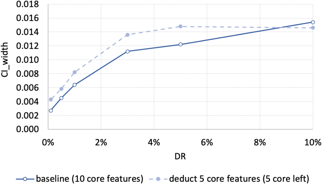
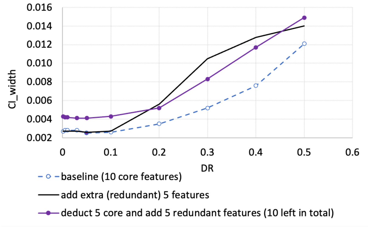
The width of the CI is proportionate to the share of the minor class, e.g., the lower the default rate (DR) is, the narrower the CI is, compare D1 to D7 (1.5% vs 0.3%) in Table A1; see also Figure 1.

When the portion of the minor class (DR) is low (below 5%), making some core features unavailable leads to the increase in the CI width (compare D3 to F3 (1.1% vs 1.3%) and D7 to F7 (0.3% vs 0.4%) in Table A1). However, when the portion is larger (e.g., 10%), we may observe reduction of the CI width (compare D1 to F1 (1.54% vs 1.46%) in Table A1).

Adding more noise (extra redundant features) widens the CI when oversampling from a very tiny class to equal proportions case (from 0.1% to 50%) (compare D16 to E16 (1.2% vs 1.4%) and F16 to G16 (1.1% vs 1.5%) in Table A1). In other cases, we do not trace neither material deterioration, nor improvement in CI width.

Oversampling to equal class shares (50:50%) mostly often leads to deterioration (CI widening) (compare D3 to D6 (1.1% vs 1.3%) and rows 1 to 2 in Table A1). However, in a realistic set-up (column G) when we know part of core drivers and also include several redundant ones, oversampling not a very minor class ( $D R \approx 3 %$ ) might improve the situation and make CI narrower (compare F3 to F6 (1.36% vs 1.28%) and G3 to G6 (1.4% vs 1.1%) in Table A1).

Oversampling the very minor class might be reasonable when considering moderate pace of resampled observations. For instance, oversampling DR of 0.1% enables to slightly reduce the CI width when the portion reaches 3–5%, but above that the CI width starts rising, compare rows 7 to 10 and 11 in Table A1; see also Figure 2.

Oversampling often leads not merely to CI widening, but also to overall model performance deterioration. As a result, CI shifts down, see Figure 3.

Figure 1.

Higher portion of minor class imply wider CI.

Figure 2.

Oversampling very minor class improves (narrows) CI, but for mild resampling.

Figure 3.

Oversampling very minor to equal portions not only widens the CI, but also drastically reduces the mean performance (shifts the CI down).

However, we do not notice material differences in the application of different CI types, all of the five ones move in tandem for both low and high initial portions of the minor class, see Figure 3.

5. Conclusion and Practical Implications

AI, in general, is nowadays thought of being an indispensable element of future progress in finance. Such progress encapsulates the proliferation of the ML models’ use for the numerous classification tasks, including the discrimination of good from bad borrowers, i.e., for the development of the probability of default (PD) models.

We show that PD model developers often face a challenge when coming across an underrepresented (minor) class. As a remedy, they solicit industry-wide practice of oversampling the minor class. This is why we focus on PD models, though our findings spread far beyond PD modeling, and are generally applicable to any binary classification task.

We manage to dig deeper into the properties of models when the underlying data is oversampled. Importantly, we show the thresholds to which it is worth oversampling the minor class given its initial portion. For instance, when the portion is moderately small one (around 3% of the total sample size), one may benefit from oversampling it to 50%. However, when the initial class is very tiny (around 0.1% of total number of observations), it might be worth oversampling only to 3-5% of the total number of entries. Moreover, we argue that such a gain in (narrowing of) confidence intervals for the PD model performance might be achieved with the trade-off by losing the overall model performance (the CI mid-value materially goes down).

We offered a statistical table which might be used by practitioners as a guide when to oversample the data or not. The enclosed programming code in Python allows gathering the equivalent answer for any combination of initial portion of the minor class, number of core and redundant features, the considered oversampling proportions.

Disclaimer

The views expressed herein are solely those of the authors. The content and results of this research should not be considered or referred to in any publications as the Bank of Russia’s official position, official policy, or decisions. Any errors in this document are the responsibility of the authors. All rights reserved. Reproduction is prohibited without the authors’ consent.

Footnotes

ORCID iDs

Yury Festa

Henry Penikas

Funding

The author(s) received no financial support for the research, authorship, and/or publication of this article.

Declaration of Conflicting Interests

The author(s) declared no potential conflicts of interest with respect to the research, authorship, and/or publication of this article.

Annex

Table A1.

Summary of Simulation Experiments.

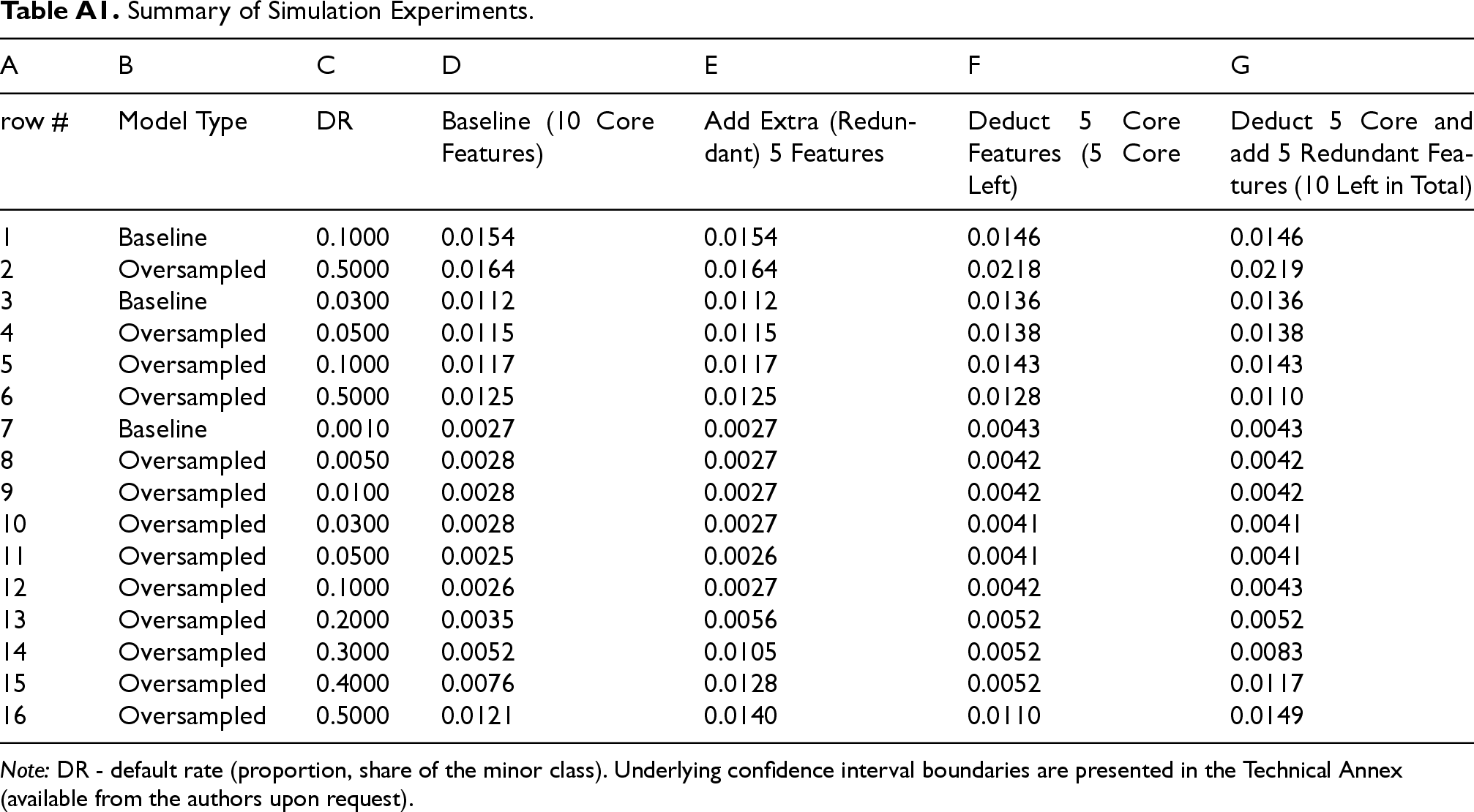
A	B	C	D	E	F	G
row #	Model Type	DR	Baseline (10 Core Features)	Add Extra (Redundant) 5 Features	Deduct 5 Core Features (5 Core Left)	Deduct 5 Core and add 5 Redundant Features (10 Left in Total)
1	Baseline	0.1000	0.0154	0.0154	0.0146	0.0146
2	Oversampled	0.5000	0.0164	0.0164	0.0218	0.0219
3	Baseline	0.0300	0.0112	0.0112	0.0136	0.0136
4	Oversampled	0.0500	0.0115	0.0115	0.0138	0.0138
5	Oversampled	0.1000	0.0117	0.0117	0.0143	0.0143
6	Oversampled	0.5000	0.0125	0.0125	0.0128	0.0110
7	Baseline	0.0010	0.0027	0.0027	0.0043	0.0043
8	Oversampled	0.0050	0.0028	0.0027	0.0042	0.0042
9	Oversampled	0.0100	0.0028	0.0027	0.0042	0.0042
10	Oversampled	0.0300	0.0028	0.0027	0.0041	0.0041
11	Oversampled	0.0500	0.0025	0.0026	0.0041	0.0041
12	Oversampled	0.1000	0.0026	0.0027	0.0042	0.0043
13	Oversampled	0.2000	0.0035	0.0056	0.0052	0.0052
14	Oversampled	0.3000	0.0052	0.0105	0.0052	0.0083
15	Oversampled	0.4000	0.0076	0.0128	0.0052	0.0117
16	Oversampled	0.5000	0.0121	0.0140	0.0110	0.0149

Note: DR - default rate (proportion, share of the minor class). Underlying confidence interval boundaries are presented in the Technical Annex (available from the authors upon request).

References

Agresti

Coull

B. A.

(1998). Approximate is better than “exact” for interval estimation of binomial proportions. The American Statistician, 52, 119–126. https://doi.org/10.1080/00031305.1998.10480550 , restricted access. https://math.unm.edu/james/Agresti1998.pdf, open access, accessed on December 30, 2023.

Altman

E. I.

(1968). Financial ratios, discriminant analysis and the prediction of corporate bankruptcy. The Journal of Finance, 23(4), 589–609.

Altman

E. I.

(2018). A fifty-year retrospective on credit risk models, the Altman Z-score family of models and their applications to financial markets and managerial strategies. Journal of Credit Risk, 14(4), 1–34. http://doi.org/10.21314/JCR.2018.243 , restricted access. https://mebfaber.com/wp-content/uploads/2020/11/Altman_Z_score_models_final.pdf, open access, accessed on December 26, 2023.

Altman

E. I.

Sabato

Wilson

(2008). The value of qualitative information in sme risk management. https://pages.stern.nyu.edu/ealtman/SME_EA_GS_NW.pdf

Audigier

Niang

Resche-Rigon

(2021). Clustering with missing data: Which imputation model for which cluster analysis method? https://arxiv.org/pdf/2106.04424.pdf. Online; accessed 15 January 2022.

BCBS (2000). Credit ratings and complementary sources of credit quality information. Working Paper No. 3. https://www.bis.org/publ/bcbs_wp3.pdf, open access, accessed on June 11, 2024.

BCBS (2006). Basel II: International convergence of capital measurement and capital standards: A revised framework - comprehensive version. https://www.bis.org/publ/bcbs128.pdf, open access, accessed on June 11, 2024.

BCBS (2017). Implications of fintech developments for banks and bank supervisors. Basel Committee for Banking Supervision Consultative Paper. https://www.bis.org/bcbs/publ/d415.htm, free access, accessed on Aug. 13, 2022.

Beaver

W. H.

(1966). Financial ratios as predictors of failure. Journal of Accounting Research, 4, 71–111.

10.

Bisogno

Restaino

Di Carlo

(2018). Forecasting and preventing bankruptcy: A conceptual review. African Journal of Business Management, 12(9), 231–242.

11.

Bräuning

Malikkidou

Scalone

Scricco

(2020). A new approach to early warning systems for small European banks. In International conference on machine learning, optimization, and data science (pp. 551–562). Springer.

12.

Brown

L. D.

Cai

T. T.

DasGupta

(2001). Interval estimation for a binomial proportion. Statistical Science, 16, 101–133. https://www-jstor-org-443.web.bisu.edu.cn/stable/2676784, restricted access. http://www-stat.wharton.upenn.edu/lbrown/Papers/2001a%20Interval%20estimation%20for%20a%20binomial%20proportion%20(with%20T.%20T.%20Cai%20and%20A.%20DasGupta).pdf, open access, accessed on December 26, 2023.

13.

Carreras

Miccinesi

Wilcock

Preston

Nieboer

Deliens

Groenvold

Lunder

van der Heide

Baccini

Korfage

I. J.

Rietjens

J. A. C.

Jabbarian

L. J.

Polinder

van Delden

Kars

Zwakman

Deliens

Verkissen

M. N.

Eecloo

Faes

Pollock

Seymour

Caswell

Wilcock

Bramley

Payne

Preston

Dunleavy

Sowerby

Miccinesi

Bulli

Ingravallo

Carreras

Toccafondi

Gorini

Lunder

Červ

Simonič

Mimić

Kodba-Čeh

OzbiČ

Groenvold

Arnfeldt

Thit Johnsen

and ACTION consortium (2021). Missing not at random in end of life care studies: Multiple imputation and sensitivity analysis on data from the ACTION study. BMC Medical Research Methodology, 21(1), 13. https://doi.org/10.1186/s12874-020-01180-y

14.

Chawla

N. V.

Bowyer

K. W.

Hall

L. O.

Kegelmeyer

W. P.

(2002). SMOTE: Synthetic minority over-sampling technique. Journal of Artificial Intelligence Research, 16, 1–26. https://doi.org/10.1613/jair.953 , open access, accessed on August 27, 2024.

15.

Chen

Marshall

B. R.

Zhang

Ganesh

(2006). Financial distress prediction in China. Review of Pacific Basin Financial Markets and Policies, 09(02), 317–336. 10.1142/S0219091506000744 . https://doi.org/10.1142/S0219091506000744, restricted access.

16.

Cheong

C. W.

Ramasamy

(2019). Bank failure: A new approach to prediction and supervision. Asian Journal of Finance & Accounting, 11, 111–140.

17.

Citterio

(2020). Bank failures: Review and comparison of prediction models. https://ssrn.com/abstract=3719997

18.

Cole

R. A.

Taylor

(2020). Predicting bank failures using a simple dynamic hazard model. Available at SSRN 1460526.

19.

Dendramis

Tzavalis

Cheimarioti

(2020). Measuring the default risk of small business loans: Improved credit risk prediction using deep learning. Athens University of Economics and Business, School of Economic Sciences Working Paper No. 12-2020. https://www.dept.aueb.gr/sites/default/files/allWP-12-20-Dendram-Tzaval-Cheimar-12-11-20_0.pdf, open access, accessed on May 31, 2024.

20.

Dunnigan

(2008). Confidence interval calculation for binomial proportions. https://www.mwsug.org/proceedings/2008/pharma/MWSUG-2008-P08.pdf, open access, accessed on May 29, 2024.

21.

Durand

Le Quang

et al (2021). What do bankrupcty prediction models tell us about banking regulation? Evidence from statistical and learning approaches. https://xtra.economix.fr/pdf/dt/2021/WP_EcoX_2021-2.pdf?1.0

22.

The Economist (2024). Can Nvidia be dethroned? Meet the startups vying for its crown. A new generation of AI chips is on the way. https://www.economist.com/business/2024/05/19/can-nvidia-be-dethroned-meet-the-startups-vying-for-its-crown, open access, accessed on May 29, 2024.

23.

Engelmann

Hayden

Tasche

(2003). Testing rating accuracy. Risk (Concord, NH), 16, 82–86. https://www.researchgate.net/publication/215991100_Testing_Rating_Accuracy, open access, accessed on December 26, 2023

24.

Europarliament (2023). EU AI act: First regulation on artificial intelligence. The use of artificial intelligence in the EU will be regulated by the AI act, the world’s first comprehensive AI law. find out how it will protect you. https://www.europarl.europa.eu/news/en/headlines/society/20230601STO93804/eu-ai-act-first-regulation-on-artificial-intelligence, open access, accessed on May 29, 2024.

25.

Fantazzini

Figini

(2009). Random survival forests models for SME credit risk measurement. Methodology and Computing in Applied Probability, 17, 29–45. https://doi.org/10.1007/s11009-008-9078-2 , restricted access.

26.

Faraj

A. A.

Mahmud

D. A.

Rashid

B. N.

(2021). Comparison of different ensemble methods in credit card default prediction. UHD Journal of Science and Technology, 5, 20–25. https://doi.org/10.21928/uhdjst.v5n2y2021.pp20-25 , open access, accessed on December 31, 2023.

27.

Feng

J. Q.

(2023). The fallacy in the paradox of achilles and the tortoise. https://doi.org/10.48550/arXiv.2310.03768. http://arxiv.org/abs/2310.03768. ArXiv:2310.03768 [math].

28.

Ferriani

Cornacchia

Farroni

Ferrara

Guarino

Pisanti

(2019). An early warning system for less significant Italian banks. https://www.bancaditalia.it/pubblicazioni/qef/2019-0480/QEF_480_19.pdf. Bank of Italy Occasional Paper No. 480.

29.

Fuster

Goldsmith-Pinkham

Ramadorai

Walther

(2018). Predictably unequal? The effects of machine learning on credit markets. https://doi.org/10.1111/jofi.13090, open access, accessed on Dec. 30, 2023.

30.

Geng

Bose

Chen

(2015). Prediction of financial distress: An empirical study of listed chinese companies using data mining. European Journal of Operational Research, 241(1), 236–247. https://doi.org/10.1016/j.ejor.2014.08.016 , https://www-sciencedirect-com-443.web.bisu.edu.cn/science/article/pii/S0377221714006511. restricted access

31.

Hanson

Schuermann

(2006). Confidence intervals for probabilities of default. Journal of Banking & Finance, 30(8), 2281–2301. https://doi.org/10.1016/j.jbankfin.2005.08.002 , https://www-sciencedirect-com-443.web.bisu.edu.cn/science/article/pii/S0378426605002128. restricted access. https://papers.ssrn.com/abstract=766345, open access (accessed on April 29, 2025).

32.

Hayek

F. A. V.

(1974). The pretence of knowledge. Nobel Lecture. https://www.nobelprize.org/prizes/economic-sciences/1974/hayek/lecture/, free access, accessed on Aug. 05, 2022.

33.

Heymans

M. W.

Twisk

J. W. R.

(2022). Handling missing data in clinical research. Journal of Clinical Epidemiology, 151, 185–188. https://doi.org/10.1016/j.jclinepi.2022.08.016 , https://www-sciencedirect-com-443.web.bisu.edu.cn/science/article/pii/S0895435622002189. open access, accessed on January 23, 2024

34.

Jabeur

S. B.

Fahmi

(2018). Forecasting financial distress for French firms: A comparative study. Empirical Economics, 54, 1173–1186. https://doi.org/10.1007/s00181-017-1246-1 , restricted access.

35.

Johnson

M. A.

Mamun

(2012). The failure of lehman brothers and its impact on other financial institutions. Applied Financial Economics, 22(5), 375–385. https://doi.org/10.1080/09603107.2011.613762

36.

Kim

Cho

Ryu

(2020). Corporate default predictions using machine learning: Literature review. Sustainability, 12, 1–11. https://doi.org/10.3390/su12166325 , open access, accessed on December 31, 2023.

37.

Kim

Cho

Ryu

(2021). Predicting corporate defaults using machine learning with geometric-lag variables. Investment Analyst Journal, 50, 161–175. https://doi.org/10.1080/10293523.2021.1941554 , open access, accessed on December 31, 2023.

38.

Kocagil

Reyngold

Stein

Ibarra

(2002). Moody’s RiskCalc

^{TM}

Model for Privately-Held U.S. Banks. http://www.rogermstein.com/wp-content/uploads/riskcalc-usbanks.pdf

39.

Kočenda

Iwasaki

(2022). Bank survival around the world: A meta-analytic review. Journal of Economic Surveys, 36, 108–156.

40.

Korol

Korodi

(2010). Predicting bankruptcy with the use of macroeconomic variables. Economic Computation and Economic Cybernetics Studies and Research, 44, 201–219. https://www.researchgate.net/publication/289639976_Predicting_bankruptcy_with_the_use_of_macroeconomic_variables , limited access

41.

Koziarski

(2021). Potential anchoring for imbalanced data classification. Pattern Recognition, 120, 108114. https://doi.org/10.1016/j.patcog.2021.108114

42.

Kristóf

(2021). Bank failure prediction in the COVID-19 environment. Asian Journal of Economics and Finance, 3(1), 157–171.

43.

Kristóf

Virág

(2020). A comprehensive review of corporate bankruptcy prediction in Hungary. Journal of Risk and Financial Management, 13(2), 35.

44.

Kumar

P. R.

Ravi

(2007). Bankruptcy prediction in banks and firms via statistical and intelligent techniques—A review. European Journal of Operational Research, 180(1), 1–28. https://doi.org/10.1016/j.ejor.2006.08.043 , restricted access.

45.

Liu

(2021). A minority oversampling approach for fault detection with heterogeneous imbalanced data. Expert Systems With Applications, 184, 115492. https://doi.org/10.1016/j.eswa.2021.115492 , restricted access.

46.

Liu

Yang

Wang

Xiong

(2022). Applying machine learning algorithms to predict default probability in the online credit market: Evidence from China. International Review of Financial Analysis, 79, 101971. https://doi.org/10.1016/j.irfa.2021.101971 , restricted access.

47.

Merćep

Mrčela

Birov

Kostanjčar

(2021). Deep neural networks for behavioral credit rating. Entropy, 23, 806–816. https://doi.org/10.3390/e23010027 , open access, accessed on May 29, 2024.

48.

Mirkin

(2016). Clustering: A data recovery approach. 2nd edition. Chapman & Hall. https://doi.org/10.1201/9781420034912, open access, accessed on Jan. 10, 2024.

49.

Moody’s Analytics (2016). RiskCalcTM Banks 4.0. https://www.moodysanalytics.com/-/media/products/riskcalc-banks-4.pdf. The publication year is not explicitly disclosed, though we may refer to the copyright year.

50.

Moscatelli

Parlapiano

Narizzano

Viggiano

(2020). Corporate default forecasting with machine learning. Expert Systems with Applications, 161, 113567.

51.

Nunes

A. R.

Morais

Sardinha

(2021). Use of learning mechanisms to improve the condition monitoring of wind turbine generators: A review. Energies, 14, 7129. https://doi.org/10.3390/en14217129 , restricted access.

52.

Obeid

(2021). Bank failure prediction in the arab region using logistic regression model. https://www.amf.org.ae/sites/default/files/publications/2021-12/bank-failure-prediction-arab-region-using-logistic-regression-model.pdf. Arab Monetary Fund (Working Paper No. 7-2021), Available online.

53.

Ohlson

J. A.

(1980). Financial ratios and the probabilistic prediction of bankruptcy. Journal of Accounting Research, 18, 109–131.

54.

Orawo

L. A.

(2021). Confidence intervals for the binomial proportion: A comparison of four methods. Open Journal of Statistics, 11, 806–816. https://doi.org/10.4236/ojs.2021.115047 , open access, accessed on May 29, 2024.

55.

Pang

Hou

Xia

(2021). Borrowers’ credit quality scoring model and applications, with default discriminant analysis based on the extreme learning machine. Technological Forecasting and Social Change, 165, 120462. https://doi.org/10.1016/j.techfore.2020.120462 , restricted access.

56.

Pereira

R. C.

Santos

Rodrigues

Henriques Abreu

(2019). MNAR imputation with distributed healthcare data. In Progress in artificial intelligence, volume 11805. ISBN 978-3-030-30243-6 (pp. 184–195). https://doi.org/10.1007/978-3-030-30244-3_16

57.

Quan

Lei

Shi

(2019). Review of bankruptcy prediction using machine learning and deep learning techniques. Procedia Computer Science, 162, 895–899. https://doi.org/10.1016/j.procs.2019.12.065 , open access, accessed on December 30, 2023.

58.

Raschka

Mirjalili

(2019). Python machine learning. Machine learning and deep learning with Python, scikit-learn, and TensorFlow 2. 3rd edition. Packt. https://www.amazon.com/Python-Machine-Learning-scikit-learn-TensorFlow/dp/1789955750, restricted access; codes: https://github.com/rasbt/python-machine-learning-book-3rd-edition, open access, accessed on Dec. 30, 2023.

59.

Rubin

D. B.

(1976). Inference and missing data. Biometrika, 63(3), 581–592. https://doi.org/10.1093/biomet/63.3.581

60.

Shibitov

Mamedli

(2019). The finer points of model comparison in machine learning: Forecasting based on Russian banks’ data. http://www.cbr.ru/content/document/file/87572/wp43_e.pdf. Online; accessed on September 08, 2020.

61.

Shrivastava

Jeyanthi

P. M.

Singh

(2020). Failure prediction of indian banks using smote, lasso regression, bagging and boosting. Cogent Economics & Finance, 8(1), 1729569.

62.

Song

Zhu

Deng

H. P.

(2021). Research on an adaptive upsampling algorithm for photovoltaic panel segmentation. Journal of Chinese Computer Science, 42, 1485–1491. http://xwxt.sict.ac.cn/EN/Y2021/V42/I7/1485 , open access, accessed on December 26, 2023.

63.

Szepannek

Luebke

(2021). Facing the challenges of developing fair risk scoring models. Frontiers in Artificial Intelligence. https://doi.org/10.3389/frai.2021.681915, open access, accessed on Dec. 30, 2023.

64.

Tian

(2017). Financial ratios and bankruptcy predictions: An international evidence. International Review of Economics & Finance, 51, 510–526.

65.

Tinoco

Wilson

(2014). Financial distress and bankruptcy prediction among listed companies using accounting, market and macroeconomic variables. International Review of Financial Analysis, 30, 394–419. https://doi.org/10.1016/j.irfa.2013.02.013 , restricted access. https://core.ac.uk/download/pdf/20482286.pdf, open access, accessed on December 30, 2023.

66.

Wilson

E. B.

(1927). Probable inference, the law of succession, and statistical inference. Journal of the American Statistical Association, 22(158), 209–212. https://www-jstor-org.web.bisu.edu.cn/stable/2276774 , open access, accessed on December 30, 2023.

67.

Yuksel

Dincer

Hacioglu

(2015). Camels-based determinants for the credit rating of Turkish deposit banks. International Journal of Finance & Banking Studies, 4(4), 1–17.