
Abstract
The Basel Committee on Banking Supervision finalized the Basel III accord in the December 2017 and launched the set of its standards – the Basel Framework – in December 2019. Both documents allow bank to use mathematical models for the credit risk estimation. There are quantitative and qualitative requirements for models to be allowed for use in the prudential regulation of banks. The approach is called an Internal-Ratings-Based one (IRB). This paper aims at discussing a set of issues related to IRB credit risk modeling and such model estimates use. Those issues include data pooling in the credit registries, applying copula-discriminant analysis, validating the borrower concentration per grade, assigning the hybrid credit rating, use of model estimates when voting at the credit committee, estimate of the ultimate credit risk-taking by banks.
Keywords
Historical background
We started discussing the credit risk modeling with Professor Sergey Aivazian around 15 years ago. At that time he supervised my Candidate of Sciences thesis. Professor Sergey Aivazian demonstrated sincere interest in the modeling finance patterns and credit risk in particular. That might have been a natural consequence that market-oriented banking started developing in Russia only during the period of the transitional reforms of 1990s. Professor Aivazian fully supported my interest in the finance area and suggested popularizing it by presenting to a larger audience. Thus I presented at the 2008 Tsakhkadzor conference launched by him, see Exhibit 1.
The Professor Fantazzini publications in the Russian Applied Econometrics journal (Fantazzini, 2008; Fantazzini, 2009) acted as the significant trigger for our finance and credit risk modeling discussions with professor Aivazian. Those articles were devoted to the world-leading practices in the credit risk modeling. Those were to a great extent induced by the requirements of the Basel Committee on Banking Supervision (BCBS). Our discussions with professor Aivazian resulted in a couple of joint publications. We reviewed the approaches to systemically important banks identification (Aivazian et al., 2011) and modeled the risk distributions corresponding to those institutions (Penikas et al., 2011). Later professor Aivazian extended his econometrics textbook with financial data applications (Aivazian & Fantazzini, 2014).
As for our paper (Penikas et al., 2011), we employed the tool most developed by professor Aivazian. This was not a conventional cluster-analysis. This was a dynamic or pattern cluster-analysis. Professor Aivazian preferred calling it a trajectory cluster-analysis. His logic came from the fact that we wish to group homogenous data trajectories. Let us illustrate his idea. Professor Aivazian always told me that first we need to decide what our objective is. More precisely, which trajectories we conceptually deem homogenous, close or adjacent. Start with Fig. 1. Trajectory A is a sinus function, B – a cosines one; C – a sinus one with a fixed downward drift. Naturally trajectories A and B are closer in levels. However, trajectories A and C – though much distant in levels – demonstrate comonotone dynamics, i.e. have equal differences, not levels.
Professor Aivazian told me that in the empirical applications we often need to deal with a interim problem setting. In real-life we do search for the trajectories neither purely close in levels, nor in differences. He argued that the most interested task is to run trajectory cluster-analysis with a weighted distance, i.e. when we assign some weight to adjacency in levels and the residual weight to adjacency in differences.
Penikas presentation at the Tsakhkadzor 2008 conference. From left to right: Professors S. Aivazian, B. Brodsky, D. Fantazzini, H. Penikas, E. Guburov.
Illustrative time series (Trajectories) data in Levels.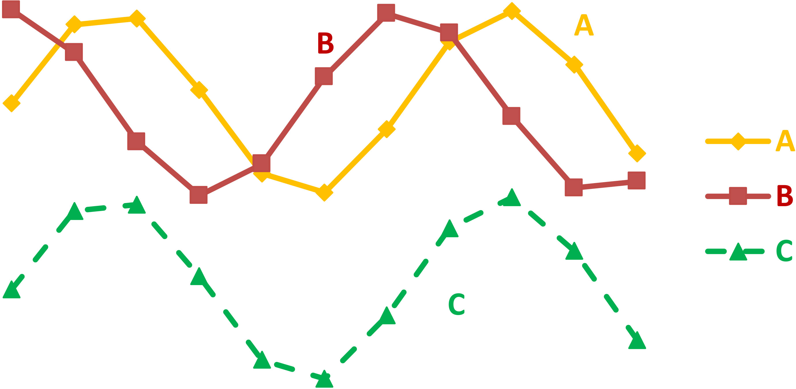
Would like to add a personal observation that describes the height of Professor Aivazian’s mathematics and econometrics knowledge. Once he presented a gift-textbook on econometrics that was offered to him from China. Of course, the entire book was written in Mandarin hieroglyphs. However, professor Aivazian told me that he understands it as disregarding the hieroglyphs, the textbook had mathematical formulas.
The objective of the current paper is to summarize various seemingly disperse issues on credit risk modeling. Each of them seems to be quite disentangled from another. However, the intent of this paper is to demonstrate how much more complicated the credit risk modeling and decision-making via the use of such models is in real day-to-day banking life.
We will try to follow the path how the decision to grant a loan originates. We briefly reintroduce the notion of credit risk and provide literature review highlights in Section 2. Then we start from the data available for credit analysis. We discuss it in Section 3. When we collected the default database, we may proceed to modeling. Conventional econometric tools – like logit, probit, discriminant analysis (linear or quadratic) – may be sufficiently improved when accounting for non-Gaussian joint distribution of default determinants. Thus, we present the advantages of copula discriminant analysis (CODA) in Section 4. When the model is ready, there are two steps: to validate the model and to assign a credit rating if it passes the validation. First, we focus on one of model validation issues, i.e. on borrower concentration per credit rating grade. We discuss this in Section 5. Second, we wish to assign a credit rating. Here there are three options whether the rating is point-in-time, through-the-cycle, or hybrid. We discuss the interrelationship of the three in Section 6. When we collected the proper data, built an accurate model, validated that there is no borrower concentration per grades, chose rating philosophy, we have everything at hand to grant the loan. However, most loans to legal entities are not automatically granted. This is the more true, the larger the loan amount is. In such cases the probability of default prediction availability is a needed, but not sufficient condition. To grant a loan ‘wisdom of (a small) crowd’ is solicited. It is a credit committee that decides upon whether to grant a loan or not. Section 7 presents consideration how to improve credit committee voting procedure using the findings from the axiomatic voting and social choice theories. When we granted the loan, we took some credit risk. The regulator wishes to evaluate the amount of the credit risk taken via the capital adequacy ratio (CAR). For the CAR purposes the loss estimates are decomposed in the expected and unexpected ones. Section 8 finishes by discussing the findings from paradigm shift, i.e. when switching from loss decomposition in CAR to total loss comparison with capital. We illustrate the findings using cases of the US and Russian banks.
Some sections present the concise review of the earlier presented materials in the form of the conference proceedings (Sections 3, 5) or a working paper (Section 4). The rest ones provide novel ideas not presented before (Sections 6, 7). Section 8 presents the extension of the previously coined idea by the author.
Credit Risk originates from the fact that the counterparty fails to meet its obligations in total or in part. It might be classified into the default risk, counterparty credit risk, concentration etc. Credit risk relates to the banking book assets, whereas the trading book ones give rise to the market risk. Credit risk may stem from both debt-type products and equity-type ones. For the latter one, please, refer to (BCBS, 2006a, pp. 344, 345), (BCBS, 2013e) as an example. World-wide credit risk forms around 84% of the total banking risks, see column (3) in Table 1. We mean the risk-weighted assets (RWA) when we say the amount of the banking risks.
Key facts on the country-wide risk allocation
Key facts on the country-wide risk allocation
At least 200 banks world-wide use mathematical models for the credit risk estimation for the prudential purposes. Such an approach is called the Internal-Ratings-Based (IRB). Basel II gave birth to it. Then it moved to Basel III with no changes from the perspective of the probability theory. Today the credit risk for at least 30% of the world banking assets, or 40% of the world GDP, is measured using IRB. For values derivation, please, refer to (Penikas, 2020c).
The probability of default (PD) is the underlying determinant of the IRB credit risk. All IRB-compliant banks need to develop PD models at least. The PD drives the value of asset correlation. It is the measure of the risks interconnectedness at the loan portfolio level. It comes from the (Vasicek, 2002) model. For the extensive discussion of this mathematical model, please, refer to (Penikas, 2020a).
PD modeling count numerous contributions. Rich reviews are available in BCBS (2000a, pp. 107–110), Kumar and Ravi (2007), Fantazzini (2008), Fantazzini (2009), Totmyanina (2011), Altman (2018), Qu et al. (2019).
We may classify the papers by the borrower type or by the loan segment:
Russian industrial companies: Dwyer et al. (2010), Totmyanina (2014), Surzhko (2014), (Mogilat, 2015), Karminsky (2015, pp. 217–222), Ermolova and Penikas (2017), Mogilat (2019). Russian banks: Peresetsky et al. (2004), Peresetsky (2012), Peresetsky (2013), Karminsky and Kostrov (2013), Fungacova and Weill (2013), Karminsky (2015), Zhivaikina and Peresetsky (2017), Shibitov and Mamedli (2019). These papers deal with the license withdrawal as data on banks defaults is not publicly available. Small and medium enterprises (SME): Altman and Sabato, (2003ca), Luppi et al. (2005ca), Pompe and Bilderbeek (2005), Fantazzini and Figini (2009), Vozzella and Gabbi (2010), Andrikopoulos and Khorasgani, (2018), Gupta et al. (2018). Project finance (specialized lending): BCBS (2001), Orgeldinger (2006), Kaluder and Augustin (2013), Morgunov (2017). Retail borrowers: Sabato (2006), Kaltofen et al. (2006), Karminsky et al. (2016). World shipping companies: Grammenos et al. (2008), Kavussanos (2014), Kavussanos and Tsouknidis (2016), Lozinskaia et al. (2017).
To become an IRB-compliant bank, it has to pass the prudential validation. The validation captures PD models. The approaches to the validation are discussed in BCBS (2005a), Moody’s (2007), Hlawatsch and Reichling (2009), Hlawatsch and Reichling (2010), Arsova et al. (2011), Maarse (2012), Yao et al. (2014), Vujnović et al. (2016), Frontczak et al. (2017), Hurlin et al. (2017), Sproates (2017), EBA (2019). Software vendors try to incorporate most of the validation statistical tests into its products (SAS, 2012).
Let us start with the data preparation stage.
The IRB approach requires banks to use at least bank specific loan default statistics. However, the bank is not limited to the internal data. He may also use external data if it demonstrates that it is representative of its own loan portfolio. Penikas (2013) suggested that using external data, its pooling with the internal one may benefit the entire economy. Thus corporate credit registries should be promoted. To get the logic underlying this proposition let us start with the methodology and proceed to the theoretical model.
Methodology
In 2013 the BCBS initiated Regulatory Consistency Assessment Program (RCAP). Its objective is to ensure the equally conservative risk treatment by various banks and jurisdictions, i.e. to ensure the level playing field (BCBS, 2013c). The BCBS started with the credit risk and offered hypothetical borrowers’ profiles to banks. It asked them to return risk estimates per those borrowers. The striking finding was that the variance of the credit risk estimates varied up to 20% in relative terms for the very same borrower (BCBS, 2013c, p. 6). There comes an objective to trace the origins of such variation and evaluate potential consequences for the economy. We specifically wish to verify whether such a variation induces dead-weight losses and how we may manage those.
Let us recall the baseline lending model of Repullo and Suarez (2000). They simplistically assume that the sales volume does not depend on the riskiness of the entity. Then consider the loan pricing given the default probability PD. Otherwise, the borrower pays back the loan and the respective interest rate
Then the optimal loan interest rate
Pagano and Jappelli (1993) claimed that the adverse selection implies higher interest rates and smaller lending volumes. Henceforth they supported the creation of the credit bureaus (registries) for the banks to share information. For instance, Powell et al. (2004) discuss optimal functioning of such bureaus. We will show below that the variation in the credit risk assessment produces similar effects as the adverse selection in the lending market. To do this, let us present the theoretical model.
For simplicity assume that there are five borrower types in our economy. Let
Now let there be two banks with the same initial capital. Borrowers may submit loan applications to any of the two banks. However, let the bank (1) has collected and approved applications from only half of the type 1 and 5 borrowers and all type 3 borrowers. Let bank (2) have collected the rest borrowers of type 1 and 5 and all the type 4 borrowers. Type 4 borrowers are riskier that the type 3 ones by construction.
The IRB approach requires banks to develop PD models at the level of homogenous portfolios of borrowers. This means that both banks would clearly differentiate type 5 borrowers as a high-risky lending segment. However, let us assume that all the residual borrowers form a sufficiently homogenous low-risk segment from the perspective of the PD model development. This implies that the mean default rate for the low-risk segment for the bank 1 is 23% and for the bank (2) – 30%.
Borrowers’ allocation in the economy
Borrowers’ allocation in the economy
Now consider the situation that type 2 borrowers apply for a loan to both banks (1) and (2). Given the discussed segmentation, the only thing banks may conclude is that those borrowers definitely belong to the low-risk segment. However, they cannot accurately know its default rate as they have no historical data for that borrower type. This means that the banks may only expect the average default rate corresponding to the low-risk segment, i.e. 23% for the bank (1) and 30% for the bank (2). Using formula (2), the bank (1) offers an interest rate of 30%; and bank (2) – an interest rate of 47%. This means that there is only a bank willing to lend at 30%, whereas there are two banks willing to lend at 47%. This means that if the type 2 borrowers require loan in excess of a single bank capacity, then the equilibrium interest rate is 47% at point A at Fig. 2.
Interest rate implications from the different data sets used for the PD model development.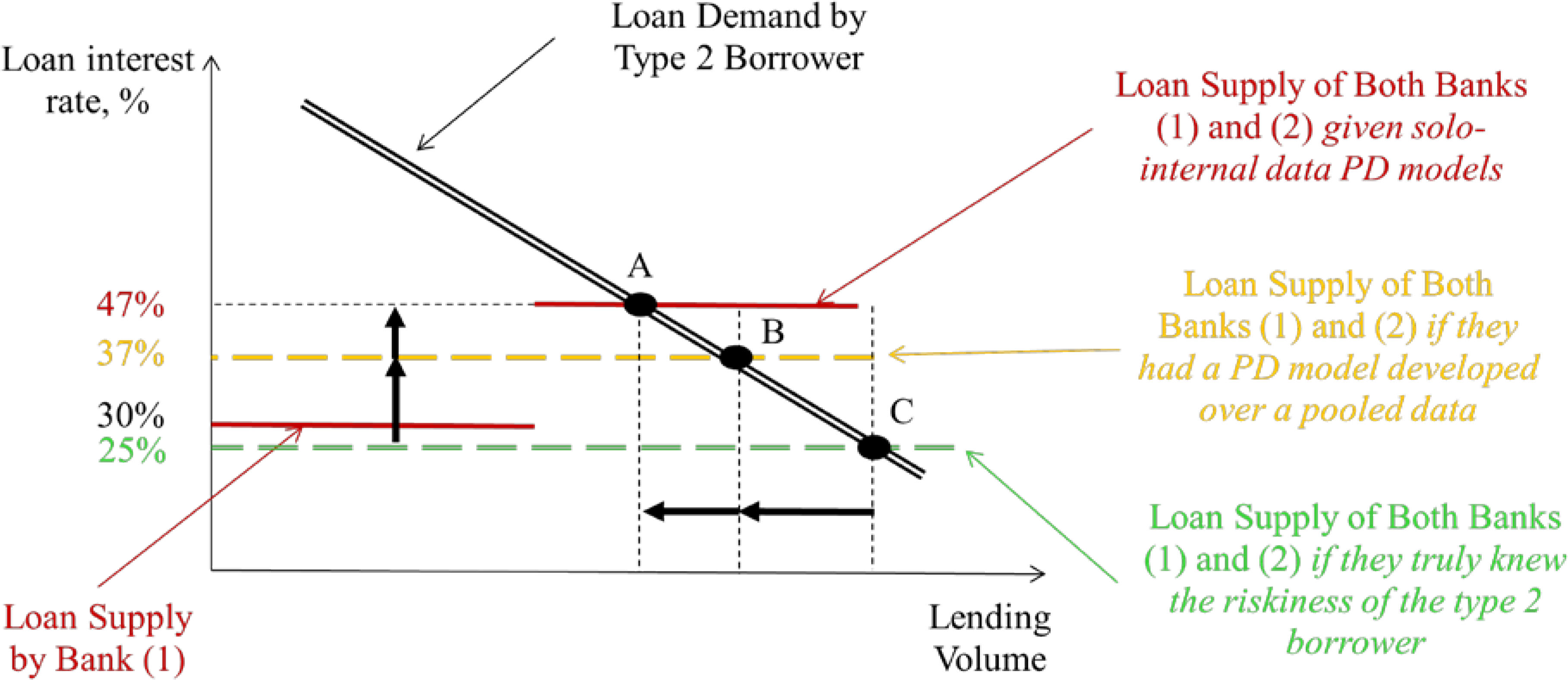
Nevertheless, if both banks had a common database – or equivalently subscribed to a common credit bureau data – each of them had data about the default experience with all borrower types except type 2. This implies that the loan supply is no more a step-wise function, but a horizontal line around the interest rate of 37%. This corresponds to a larger lending volume in point B. For comparison, if both banks knew the true default rate of the type 2 borrowers, they could offer a loan at a larger volume and at a lower interest rate of 25% in point C.
Thus, Penikas (2013) recommends the regulator to:
Promote public credit registries, including for the legal entities as is present in France (Banque de France, 2006); and Recommend developing PD models at a larger data set, i.e. prefer data pooling. This corresponds to the BCBS recommendation to avoid low-default portfolios (LDP) BCBS (2005b) and the recommendation from Penikas (2020b) to avoid regulatory arbitrage stemming from the LDP.
Penikas (2013) expects that the data pooling in the credit registries and PD models development on those ones would decrease the dead-weight losses when running IRB and improve the social welfare. Let us proceed to the PD modeling stage.
Section 2 has a list of papers dealing with the PD model development. Most of the papers use logit, probit, linear or quadratic discriminant analysis (DA); others apply machine learning techniques, including neural networks. Those approaches are sufficient when the joint PD determinants’ distribution is multivariate Gaussian. However, when this is not the case, we need to look for an alternative. Khankov and Penikas (2015) demonstrate the advantages of using copula Discriminant analysis (CODA) in such a case.
Literature review
Default is a flag assigned to a borrower or facility. Genest and Neslehova (2007) do not recommend applying copulas to count data, including binary one. They worry of the copula non-unique identification. To overcome such a limitation, we should look closer to the copula-discriminant analysis (CODA).
Sathe (2006) seems to have coined the CODA approach. He looked at two copula identification approaches: EML (Exact Maximum Likelihood) and CML (Canonical Maximum Likelihood). EML stands for the simultaneous estimation of copula and marginals’ parameters. CML suggests decomposing estimation in two steps. First, the marginals are modeled. Second, copula is fitted. Khankov and Penikas (2015) develop CML approach.
Sathe (2006) suggested the following modification of the DA maximum likelihood formula:
Han et al. (2013) suggested their own approach and were the first to call it Copula Discriminant Analysis (CODA). They theoretically justified the Gaussian-copula-based CODA. They demonstrated its advantages over the linear DA and logit model.
Bivariate scatterplots for the various combinations of copulas in default and non-default classes. Source: Khankov and Penikas, (2015).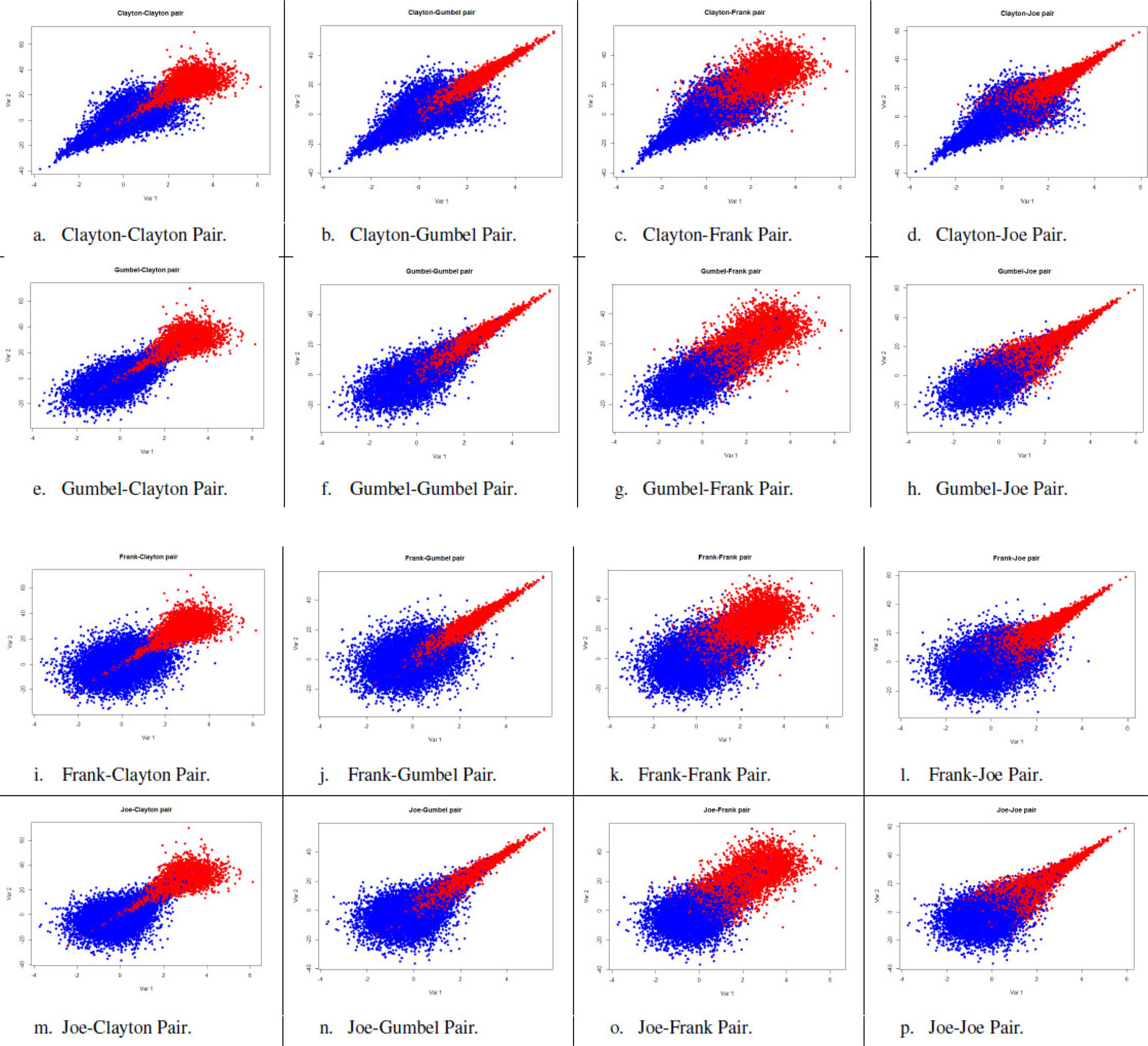
In parallel to Han et al. (2013), Scheungrab (2013) extended the approach by Sathe (2006). She used kernel estimates for the marginal distributions and vine copulas to proceed with the joint ones. She did not come to a significant advantage of CODA versus alternative methods, in contrast to Han et al. (2013).
That is why Khankov and Penikas (2015) wish to investigate earlier undiscussed CODA properties when applying to PD model development. They wish to calibrate CODA accuracy in PD prediction subject to:
Sample size; Default rate and, especially, the case of low-default portfolios; Initial variation of joint distribution by classes of default and non-default observations.
Latter issue came from Fantazzini (2009). He argues that marginals are much more important than copula when modeling joint distribution. Let us describe the methodology of Khankov and Penikas (2015).
Khankov and Penikas (2015) call their approach LL-CODA where LL stands for the LikeLihood. Below we describe its steps:
We fit the marginal distributions for the artificial PD determinants at the training (validation) dataset. We obtain the cumulative distribution functions. Then we fit copula parameters for the four copula families: Clayton, Gumbel, Frank, Joe. We proceed with the copula that demonstrates the largest likelihood function value. We compute the logs of a priori odds for the default and non-default classes in the training set. At the testing (examination) set we compute the log likelihood function values for each observation, i.e. per each combination of artificial PD determinants using the marginals and copula fitted at steps 1–4. We allocate the observation to a class based on the value of the likelihood function.
Khankov and Penikas (2015) base their calibration on bivariate distributions. Red dots stand for the artificial defaults. Blue ones – for the non-defaults. The two dimensions of the bivariate distributions could be the debt level (debt-to-equity) on the horizontal axis and the accounts receivables in total assets on the vertical axis. The larger each of the two indicators is, the more likely the borrower is to default on its loan taken.
They start with 16 joint distributions. Each has 2 mln observations, see Fig. 3. For simplicity, marginals differ by classes only in the mean values. The difference in means equals to the two standard deviations. Marginals are different for two PD determinants. We model those as Gaussian distributions.
Findings
First, we wish to identify which copula combinations result in the highest PD prediction. Figure 4 presents three accuracy indicators: hit rate (blue column), type I (orange column) and II errors (grey column). Type I error stands for rejecting the null hypothesis, i.e. expecting the borrower is creditworthy when this is not the case. Type II error corresponds to accepting the alternative one, i.e. believing the borrower is not to payback when it has sustainable future cash inflow.
We wish to remind that the LL-CODA approach could have chosen out of the four copulas initially used for data simulation. A natural finding is that the highest discrimination – or PD prediction accuracy – corresponds to the cases where we can visually easy differentiate the default and non-default class observations. For instance, compare the largest hit rate of 95.36% for a. Clayton-Clayton (C C); or 94.88% for j. Frank-Gumbel (F G); and the lowest of 92.01% for g. Gumbel-Frank (G F); and 91.03% for p. Joe-Joe (J J), see Fig. 4a.
Average prediction accuracy indicators for the LL-CODA approach. Source: Khankov and Penikas (2015). 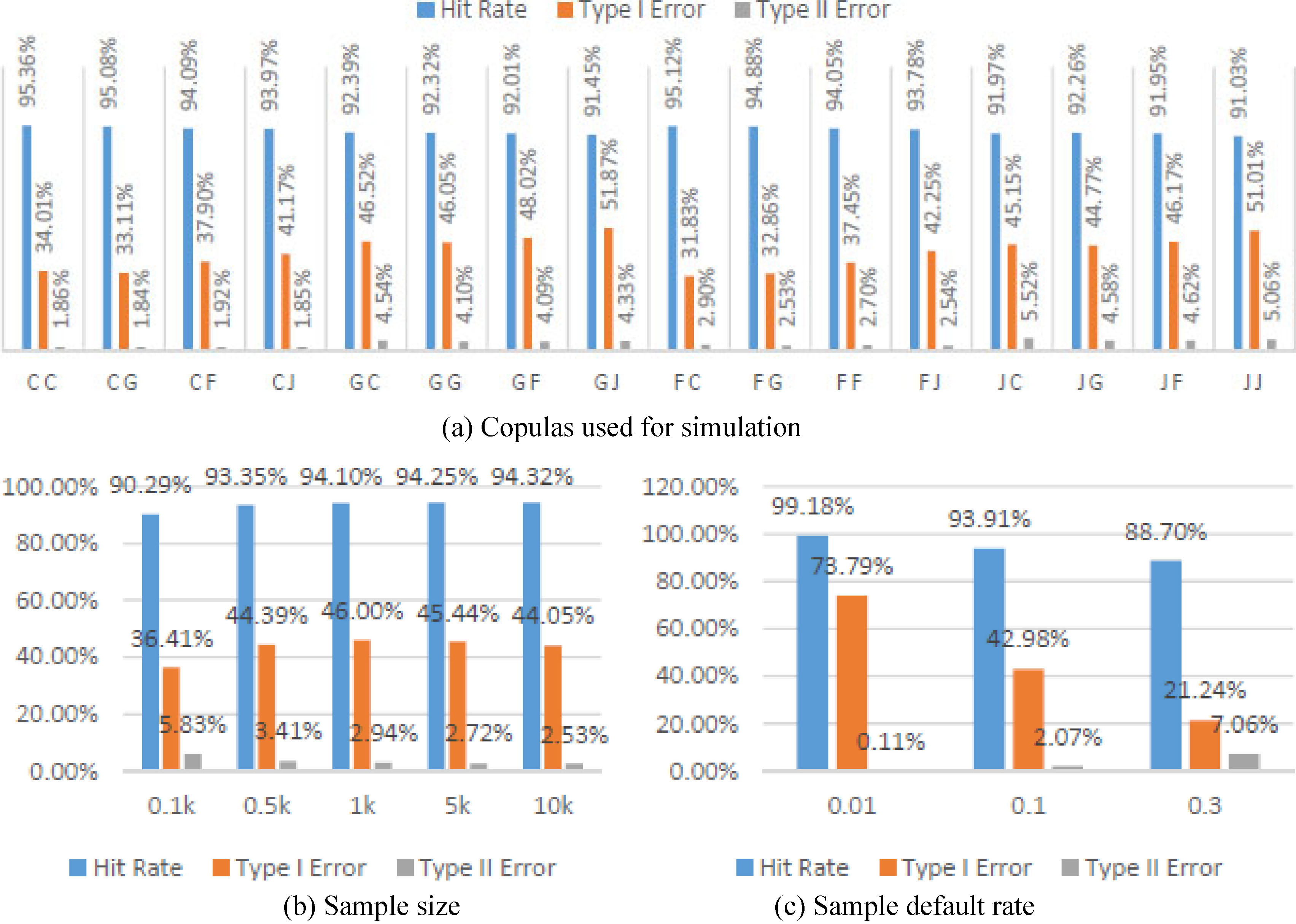
Type I error varies more by cases. Compare the best case of 31.83% for i. Frank-Clayton (F C); and the worst of 51.87% for h. Gumbel-Joe (G J). Type II error varies not that much, though it moves in the same direction hitting the best minimum value of 1.86% for a. Clayton-Clayton (C C).
Khankov and Penikas (2015) then proceed with the deeper investigation of only four cases:
Clayton-Clayton – as the easiest one to disentangle defaults from non-defaults; Joe-Joe – as the worst one, i.e. it is most difficult to differentiate; and Gumbel-Gumbel and Frank-Frank as interim cases by complexity to discriminate defaults from non-defaults.
Figure 4b presents the accuracy calibration subject to sample size. The highest accuracy level is achieved for 500 observations (borrowers). When we expand the dataset more, there is no dramatic rise in PD prediction accuracy.
Figure 4c presents LL-CODA calibration subject to default rate in the dataset. From the first glance, it may seem that the lower default rate corresponds to the highest accuracy level. However, this comes from the fact that the dataset is dominated by a single borrower type (non-defaults). When we dig deeper into the accuracy of defaults prediction, we regret to observe that only
However, even when the default rate equals to 10% the type I error is 40%. This is quite high. We wish it were lower. However, we cannot claim that this is a LL-CODA deficiency as the competitive DA approaches deliver comparable results.
Let us discuss the impact of marginals and copula for the PD prediction accuracy. We expected that large sample size enables us to correctly fit the copula based on likelihood function maximization. Hence, we wished the classifier in such a case to deliver the most accurate predictions. Our expectations came true only in part.
In most cases the copula families were identified correctly. For instance, for the non-defaults copula was always correctly fitted. As for the defaults, copula fit correctness depended much upon the combination of copulas in two classes, upon the sample size and sample default rate. On average LL-CODA correctly identified copula for the 88% of the defaults classes. When the sample size rose to one thousand observations, the proportion approached 100%.
Though LL-CODA performed quite well in identifying copula family, it failed much in properly identifying the copula parameter. When the sample size and default rate rise, the parameter estimates converge to the true values. However, the standard errors do not decrease that fast. This results in lowering of the t-statistics corresponding to copula parameter estimates. Thus data pooling may not always imply higher precision of the copula parameter estimates.
We departed from CML for the LL-CODA by maximizing the likelihood function. However, there came situations when fitting improper copula resulted in higher PD prediction accuracy. As this seems counterintuitive, we wish to have a method that correctly fits the data and has high PD prediction accuracy. That is why, Khankov and Penikas (2015) try to choose the copula by optimizing one of the three prediction accuracy indicators.
Figure 5 provides the results. Approach minimizing the type I error (T1-CODA) outperforms the rest. We should recall that this indicator is the most important out of the three for a bank granting a loan. So far, T1-CODA has the lowest average type I error of 34.6%, whereas for the LL-CODA it is 39.6%; and 42.9% for the linear DA. Hit rate indicator is comparable out of the three approaches: it is 92.4% for the T1-CODA, 92.7% for the LL-CODA and 92.1% for the LDA. That is why T1-CODA should be preferred to the LL-CODA.
The proportion of situations when there is the highest classification accuracy. Source: Khankov and Penikas (2015).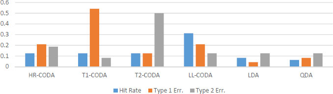
We wished to analyze the CODA method sensitivity to the number of defaults. That is why we fixed the default rate at 10% of the total observations. We varied the number of observations from 50 to 500 with a step of 50. There were 5 to 50 defaults, respectively. The median hit rate for the LL-CODA is 92.65%. This is higher than for the benchmarked methods, see Fig. 6. However, the type I error is quite volatile for it and its median is the highest. For comparison, it is 53% for the LL-CODA, 37% for the T1-CODA, 47% for the linear DA and 44% for the quadratic DA, see Fig. 7.
Benchmarking CODA against linear and quadratic da. Source: Khankov and Penikas (2015).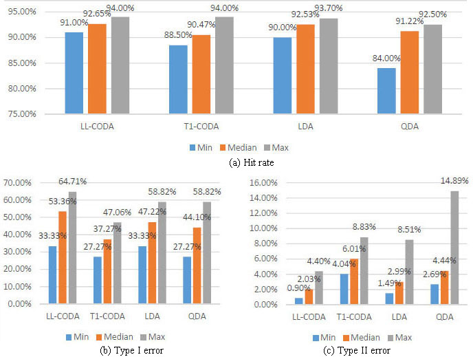
Sathe (2006) suggested copula incorporation into the discriminant analysis (CODA). Khankov and Penikas (2015) have reconfirmed that CODA has advantages over the conventional discriminant analysis (DA) when the joint PD determinants have non-Gaussian distribution. The novelty of Khankov and Penikas (2015) is that they have demonstrated that the highest PD prediction accuracy is achieved when the number of observations exceeds 500. Same time, though small sample experience does not deliver satisfactory results, CODA outperforms the DA tools. Sample default rate is important for the PD accuracy prediction. For instance, Khankov and Penikas (2015) show that CODA is unsuitable for the low-default portfolios. More importantly, Khankov and Penikas (2015) demonstrate that a bank should prefer using CODA by minimizing type I error, rather than my merely maximizing the likelihood function.
When we have shown how to derive a more accurate PD prediction than the conventional models suggest, we are able to assign a credit rating to a borrower.
Small sample CODA accuracy performance. Source: Khankov and Penikas (2015). 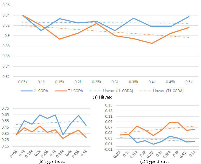
Problem setting
When the bank runs IRB, the BCBS requires it to assign a credit rating. The rating is usually base on a quantitative PD model of a type discussed in Section 4. However, BCBS prescribes that the number of credit grades equals to seven for the non-defaults and one is left for the defaults, i.e. the total number of grades should be eight at least (the Master Scale design). Having introduced such a requirement, regulator verify whether there is no excessive credit rating grade concentration. The below Herfindal-Hirshmann index (HHI) acts as a concentration measure.
ARB (2013, pp. 60–61) has the acceptance criteria. HHI value in excess of 20% is a yellow (satisfactory) validation zone; 30% is a red (unacceptable) one. EBA (2019, p. 26) recently suggested that the grade concentration does not rise without imposing any quantitative thresholds.
Ermolova and Penikas (2019) challenged the origin of the eight grade requirement and the sufficiency of the above quantitative threshold for the HHI value.
We were unable to trace the roots of both requirements. That is why we wish to offer three suggestions on its probable origin.
First, if a bank wishes to run IRB using default statistics only without borrower details, the larger number of grades enables to better differentiate the borrowers by allocating new applicants to various and not to a single (average) credit rating grade.
Second, the requirement to have no credit rating concentration may follow from the need to have a through-the-cycle (TTC) credit rating philosophy. For instance, Oyama and Yoneyama (2005, p. 11) suggest that volatile point-in-time (PIT) ratings would result in borrower proportions’ fluctuations. In times of boom there are many low-risk-assigned borrowers, whereas during the crisis most would fall to the high-risk grade. In case the models are TTC than they should deliver credit ratings that are stable throughout the economic cycle. Then Oyama and Yoneyama (2005, p. 11) expect that all the credit ratings are more or less equally presented in the loan portfolio, i.e. they talk about uniform distribution. This does not imply that the bank should definitely finance borrowers with 100% PD estimate. It should not, but in any loan portfolio there should be better and worse borrowers, and they should be equally distributed in the range on the PD approved in the bank credit policy, e.g. below 20% for corporate borrowers. This means that a requirement to have no concentration in no less than eight credit rating grades acts as a sort of a sanity check whether the IRB framework of a bank is a TTC one. However, we remember Ozdemir and Miu (2009) who claim that purely TTC rating systems do not exist.
Third, if we got the idea on the origin of the requirement, we wish to reverse engineer the origin of the quantitative threshold. Let us then compare several loan portfolios with various borrower distributions by loan exposure, see Fig. 8.
Increase in the number of grades enables to reduce grade concentration in HHI terms.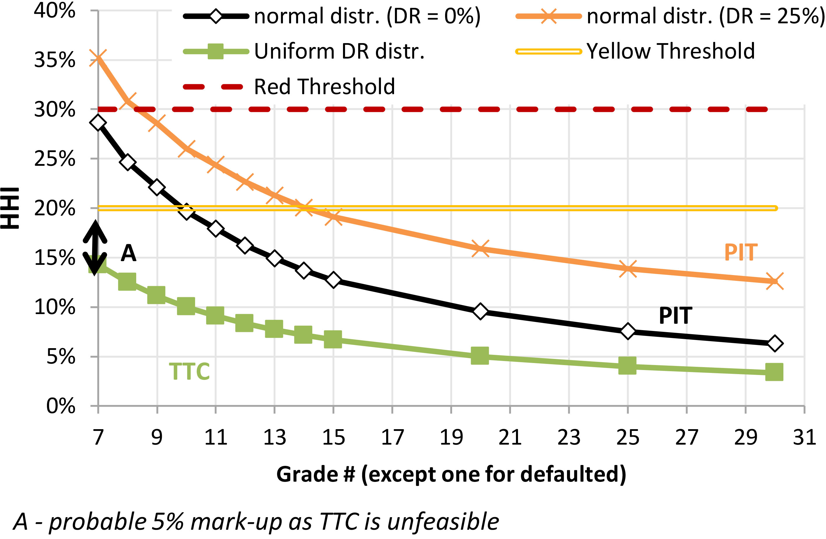
Black line at Fig. 8 corresponds to the normal distribution of borrowers by seven non-defaulted credit rating grades. As we may see, HHI than equals 30%. This is exactly the red threshold used in the IRB validation. This is the first novelty of Ermolova and Penikas (2019) as no one previously demonstrated the origin of the threshold value.
The second novelty of Ermolova and Penikas (2019) is that they show the insufficiency of the fixed validation criteria when the bank may increase the number of the rating grades. The idea is simple. The HHI stands for the concentration measure. We wish that the Master Scale design does not change the measure of concentration. Otherwise it is a manipulation, or a regulatory arbitrage. Other cases of regulatory arbitrage are discussed in Ferri and Pesic (2017), Penikas (2020a), Penikas (2020b).
However, as one may see from Fig. 8 the more the number of credit rating grades is, the lower the HHI value is. It means that if a bank wishes to pass the IRB prudential validation, but wishes to make no material changes to its lending strategy given highly concentrated by grades portfolio, all it needs is to increase the number of grades in the Master Scale.
The implication for the regulator here is suggested in Ermolova and Penikas (2019). The quantitative threshold should decrease proportionate to the rise in the number of the credit rating grades as in Fig. 8. For instance, if there are 21 grades, the red threshold should be 10%, and not 30%.
We have discussed the proper approach to validating the credit rating grade concentration. We supposed that the requirement may originate from the need to have a TTC rating philosophy. However, there is a question how to obtain one or at least a somewhat hybrid one.
We already mentioned that there are two approaches to the credit rating assignment, i.e. two rating philosophies. They are described in greater detail in Ozdemir and Miu (2009). Conceptually we may present them at Fig. 9. PIT credit risk estimates are volatile. PDs are low in the economic boom times and high during the crisis. Volatile red line with markers corresponds to it. TTC estimates are, on opposite, quite stable. Horizontal black line reflects it. Quite often the mean historical default rate is considered as the TTC PD proxy, or the central tendency (CT).
When one may hear that a hybrid PD (
where
Credit rating philosophy comparison.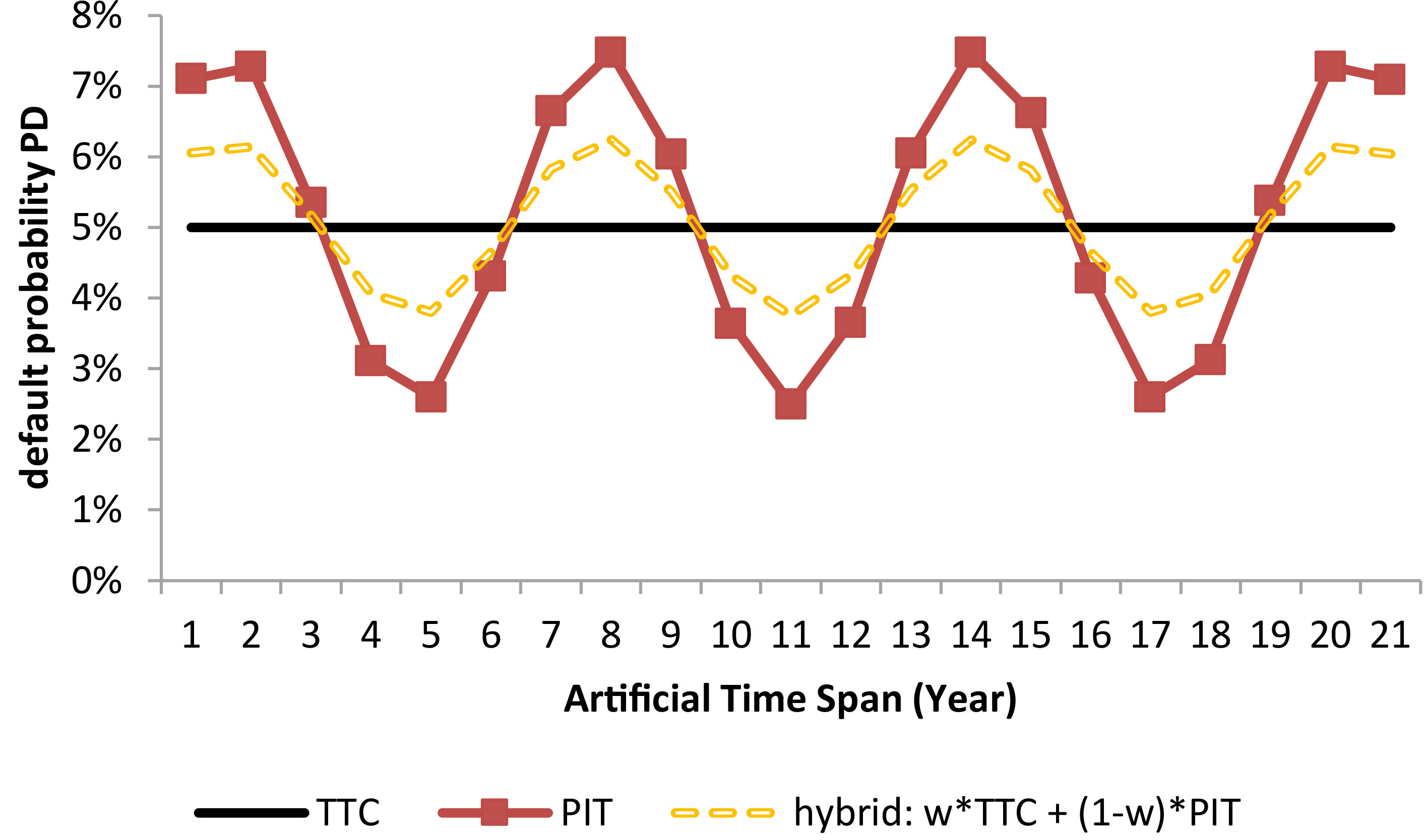
The only question here is how to define the
We discussed which data to use for PD model development, how to do it and validate one, how to arrive at the appropriate credit rating. Now we have everything at our disposal to make the decision. However, this is not automatic and there is a separate domain of model application, or the model Use Test (BCBS, 2006b). We discuss it in the next section.
As a response to the global financial crisis of 2007-09, the BCBS suggested a review of remuneration policies. Inter alia it proposed to introduce variable and deferral parts. Banks should link those parts to the risk indicators (BCBS, 2011). However, BCBS spoke nothing about the decision-making process itself, though it is exactly the collective body (a committee) that often decides upon large sum loans. Besides, implementing the proposed restrictions, the bank managers may choose one of the two distinct ways: either to gamble and take on excessive risk or to be as passive as possible, not to lose the accumulated bonuses. Latter may result in overly cautious behavior when no one wishes to grant any loan (to approve any loan application). Same time the bank shareholders wish loans to be granted to cover the operational costs at least and to meet earnings targets at best. This means that we need to design the proper procedure for the voting at the credit committee.
One may wish to remember the axiomatic voting theory and the social choice one (Maskin, 2020). Those focus on the properties of the voting rules, including their manipulability. Some common rules are simple majority (it is often used at the bank credit committees), weighted majority, absolute majority, Borda rule. For instance, Aleskerov et al. (2019) discuss 14 rules. Young (1995) claims that the maximum likelihood-based voting should be preferred; Aleskerov et al. (2019) – Hare rule; Maskin (2020) – Borda rule. However, to the best of author’s knowledge, there is no discussion of optimal voting rule in the credit committee.
The author contribution here is the proposal to shift from the simple majority when voting for a loan to a weighted majority. This rule is mentioned by Young (1995, p. 53). Its idea is to assign higher voting power to the systematically accurate credit voter. Here it is not that important what the preferences of the voter are with respect to the numerous loan applications, but how accurate he predicts which may be redeemed and which – may not. By the way both decisions are important: to grant and to reject the loan application. Upstanding does not add to voter’s accuracy. Using weighted-majority voting rule is in fact the use of the time series forecasting approach for combined forecasts (Teruia & van Dijk, 2002; De Pooter, Ravazzolo, & van Dijk, 2010; van Dijk & Franses, 2019). The idea is to assign the larger weight to a model that is inversely proportionate to the root mean squared prediction error (RMSPE). The larger RMSPE is, the lower weight is assigned to such a model, or a voter in terms of a credit committee.
We have discussed preparation to loan application review and decision-making upon it. When it is approved, the bank takes on the risk. The universe of the credit risks taken is reflected in the capital adequacy ratio. Penikas (2020a) discussed the vulnerabilities of a ratio as a measure when the total risk estimate is decomposed into expected and unexpected values. Let us look at the quantitative application suggested in the paper.
Credit risk taking: Shift from CAR to K versus total risk comparison
Penikas (2020a) has demonstrated that the capital adequacy ratio (CAR) can be written as a comparison of total capital and total risks, i.e. there is an equivalent transition from Eqs (7) to (8).
where
Shift to no risk amount decomposition for the russian D-SIBs.
Though the transition from Eqs (7) to (8) is equivalent, using the buffer from Eq. (8) may provide insights that are unavailable from the CAR perspective. To demonstrate it let us look at the publicly available data for the Russian domestic systemically important banks (D-SIBs) and the selected American global ones (G-SIBs). Results are available in Figs 10 and 11, respectively for April 2020 data.
If we look at the CAR for the total capital of the Russian Banks, the Gazprombank (GPB) and VTB possess the lowest values. The lower the CAR value is, the more credit risks the banks has taken. This was always thought prior to Penikas (2020a). Actually, when we transit to the capital buffer in the form of Eq. (8), we see that the ranking of the Russian banks dramatically changes. For instance, the lowest buffer is with the Otkrytie (Open) and Promsvyazbank (PSB). Those two banks were recently taken under direct supervision of the Bank of Russia because of material losses incurred in the prior periods. Looking at the conventional CAR measure of the type Eq. (7) did not allow us to trace the problem banks. Using formula Eq. (8) permitted us to do it.
Shift to no risk amount decomposition for the selected US G-SIBs.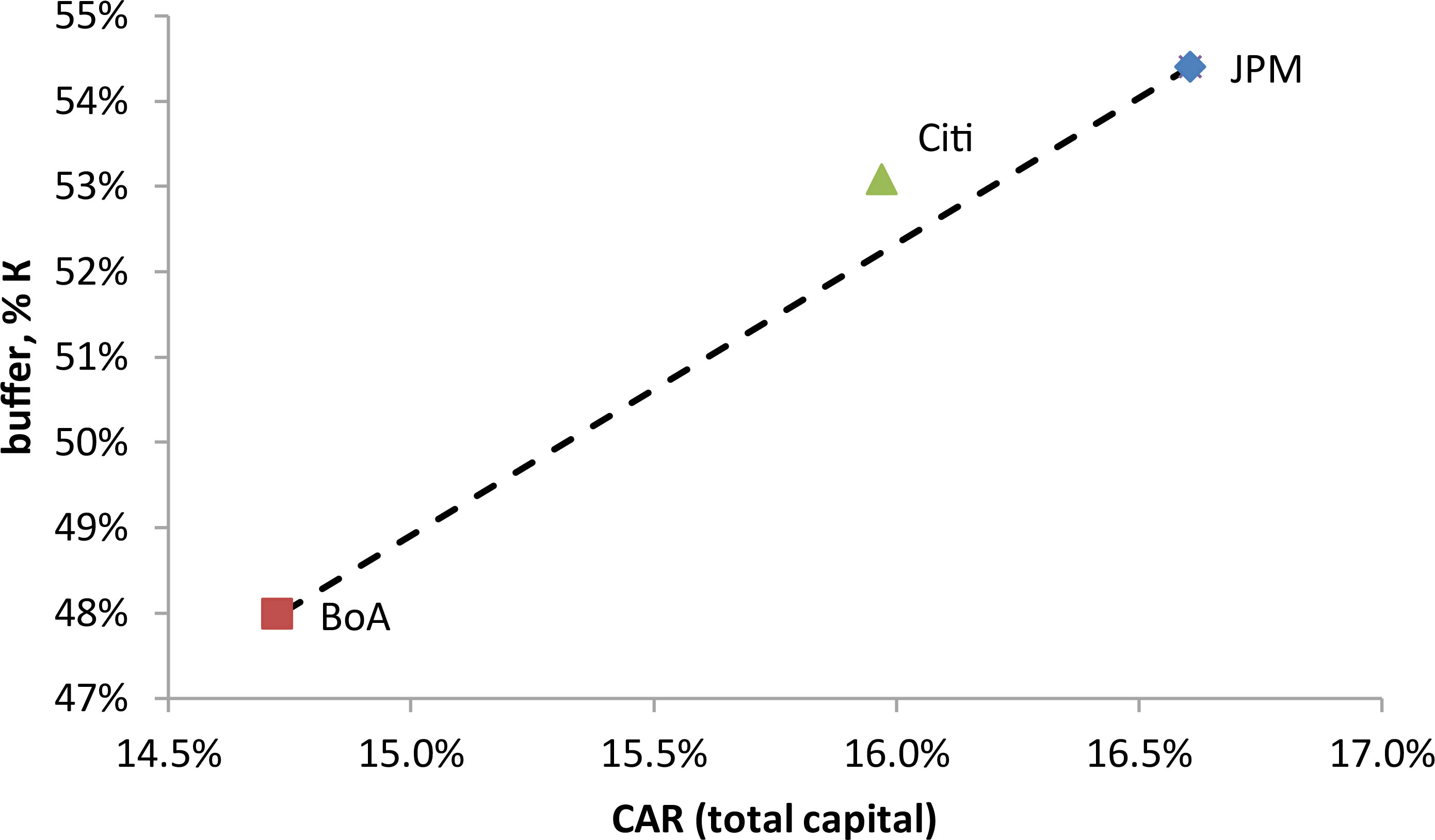
To cross-check our approach, we looked at the US banks’ 2019 annual data: JP Morgan (JPM), Citibank (Citi), Bank of America Merrill Lynch (BoA). The capital buffer from Eq. (8) is comparable for all three banks. It is around 50%. This is higher than the average for the Russian D-SIBs. When we look at the US banks we do not see a shift in ranking as we do with the Russian ones. However, if we join the dots at Fig. 11 for the two extreme banks, we may see that Citi bank is positively distinguishable of them. It lies above the dotted line. This means that it has larger capital buffer in terms of Eq. (8) compared to an average of its peers.
The Basel Framework is a collection of the banking prudential standards. It was adopted on December 2019 and has around 1.8 k pages. One of its sections allows banks using default statistics and mathematical models to compute the prudential ratio of capital adequacy (CAR). In brief, it requires having a probability of default (PD) model and an ‘engine’ where to put it as an input. Many papers dealt with PD model development. We listed them in Section 2. Many criticized the ‘engine’ – the underlying Vasicek model. The discussion of the accumulated criticism is available in (Penikas, 2020a). Those critical points are not considered in the Basel Framework.
However, this paper demonstrates that there are other important issues, solutions and methods worth considering in order to arrive at the more accurate credit risk assessment and more sustainable banks.
That is why this paper is novel in that:
It proved that developing PD models at the pooled (credit bureau) data is lucrative for the society and should be promoted; Minimizing type I error enables to increase PD prediction accuracy when the joint distribution of PD determinants is non-Gaussian and copula discriminant analysis (CODA) is used; One should use a decreasing HHI threshold for the larger number of credit rating grades to validate the absence of borrower concentration per grades; The TTC and hybrid ratings devalue the benefits of the PD model accounting for the borrower and facility characteristics. That is why we wish a regulator promotes using PIT PD estimates for the IRB; As a part of the PD model use test, the credit committee voting rule based on the PD estimate should be changed. The weighted majority rule should substitute a simple majority one to increase the accuracy of decision-making upon whether to grant a loan or not with the given PD prediction. We have shown how the shift from CAR to no decomposition of losses into the expected and unexpected ones enables to raise the information value of the risk measure to the bank stakeholders. As for the Russian largest banks, we revealed the previously unobserved changed in the ranking of the banks’ financial standing. As for the US banks, we were able to demonstrate the relatively larger capital cushion of Citibank against its two peers.