Motion process monitoring using optical flow–based principal component analysis-independent component analysis method

Abstract

In this article, for the first time, the optical flow and principal component analysis followed independent component analysis are combined for monitoring the motion process of robotic-arm-based system. Two kinds of optical flow, namely dense optical flow and sparse optical flow, extracted from each two successive frames of motion process in forms of video stream are used as the samples of motion-related variables of principal component analysis–independent component analysis algorithm. Relative work illustrates the effectiveness of principal component analysis–independent component analysis method for non-Gaussian process monitoring. The proposed dense optical flow–principal component analysis–independent component analysis and sparse optical flow–principal component analysis–independent component analysis algorithms use three-way array as their data which follows non-Gaussian distribution. Data unfolding, data normalization, and proper definition of the control limit are introduced. Based on dense optical flow–principal component analysis–independent component analysis and sparse optical flow–principal component analysis–independent component analysis algorithms, the corresponding motion process monitoring scheme is developed, and a case study of robotic-arm-based marking system is taken to evaluate the performance of these methods. The results demonstrate the capability and efficiency of the proposed methods.

Keywords

Principal component analysis independent component analysis motion process monitoring fault detection robotic-arm-based marking system

Introduction

More and more robotic arms are applied in industry for improving product quality and reducing product cost. For safety and quality reasons, monitoring the motion process of the robotic arm and its surrounding is of great demand.^1–2 Traditionally, monitoring the motion process of robotic arm is performed by analyzing the data collected by sensors attached to the joints or surface of the robotic arms.³ There are some defects of this method: (1) when some key sensors or all the sensors are broken down, monitoring cannot be performed, (2) sensors can collect only the data of robotic arm itself and cannot be sensitive to other surrounding objects’ motion which can be latent faults sources of the robotic arm, and (3) human appears in the dangerous area of robotic arms’ working range which risk their life. Therefore, the design of motion process monitoring method for solving these problems is of great significance. Data-driven multivariate statistical process monitoring (MSPM) methods have been widely used to capture the characteristics of the process for further establishing accurate and reliable monitoring model,^4–10 such as principal component analysis (PCA) and partial least squares (PLS). However, there is a pre-assumption that the data follow Gaussian distribution which can be hardly satisfied in practical application. Independent component analysis (ICA), which reveals higher-order statistical information of the process data, is widely used in coping with non-Gaussian process.^11–18 Various methods and successful applications are reported based on PCA-ICA. For example, Berg et al.¹⁹ proposed PCA-ICA to extract Gaussian and non-Gaussian information for blind source separation. Huang and Yan⁹ discussed to use variable distribution characteristic (VDSPM) which employs D-test to separate the Gaussian subspace and non-Gaussian subspace. Jiang et al.¹⁰ introduced a PCA-ICA integrated with a Bayesian fault diagnosis method for non-Gaussian process. Megahed et al.²⁰ published a review on image-based process monitoring methods, which are divided into several groups including multivariate and profile-based techniques, spatial control charts, and multi-variate-image-analysis (MIA) control charts. In the first group, multivariate control charts along with a feature extraction method and profile modeling were used for process monitoring. Wang and Tsung²¹ modeled the relationship between a sampled image and a baseline using Q-Q plots and then used profile-monitoring methods to detect changes in these plots. A major disadvantage of this method is that it ignores the information about pixel locations. The spatial control charts, however, consider the spatial information using non-overlapping windows that move across an image.²² The main disadvantage of profile-based and spatial monitoring methods is that these methods are typically applicable to grayscale images and they cannot be directly used for the monitoring of color images. MIA techniques, on the other hand, can handle color images by extracting features from each color channel. Although MIA can effectively extract color features, it neglects the spatial information of an image.²³ However, new issues in process monitoring arise when it comes to motion process monitoring using vision data captured by a fixed camera which is independent to the process. What kind of feature of the video frames can describe the motion information of the objects in the scene? How to deal with the motion-related feature to model the normal motion process for monitoring has become a challenging problem.

The optical flow is the pattern of apparent motion of objects, surfaces, and edges in a visual scene caused by the relative motion between a camera and the scene. The optical flow information is widely used in image processing and navigation including motion detection, object segmentation, motion compensated encoding, and stereo disparity measurement. Various methods are proposed for calculating the optical flow.^24–28 In present article, the optical flow is calculated through two successive frames of a video, and two kinds of optical flow are employed, which are dense optical flow (DOF) and sparse optical flow (SOF). DOF uses every pixel between the two successive frames for calculating the optical flow field. However, SOF only uses some feature points, corner points for example, and search for the same points in current frame for velocity. Obviously, DOF gives DOF field, but needs more computation than SOF.

Based on DOF and SOF, we propose DOF-PCA-ICA and SOF-PCA-ICA methods for monitoring motion process of robotic-arm-based system. Normal motion is captured by fixed camera in form of video stream, and the DOF and SOF are extracted from the video stream for modeling. Unlike traditional MSPM method, the data of DOF-PCA-ICA and SOF-PCA-ICA are a three-way array and motion-related variables follow non-Gaussian distribution. Three-way array is a useful tool, which has been used by the multiway principal component analysis (MPCA) for traditional sensor monitoring for batch process. Data unfolding with normalization needs to be done for performing PCA-ICA algorithm. The control limits of I² statistic for monitoring cannot be determined using approximate distribution function. Kernel density estimation (KDE) method is an effective tool of estimating the distribution of random variable. In this study, we adopt KDE method to determine the upper control limits of the monitoring statistics. Finally, based on DOF-PCA-ICA and SOF-PCA-ICA, the corresponding fault detection approaches are developed to monitor robotic-arm-based marking system (RABMS) motion process. The results of the proposed monitoring methods show satisfactory monitoring performance.

The remainder of this article is organized as follows. A brief review of optical flow extraction and PCA-ICA algorithm is presented in section “Preliminaries.” Detailed descriptions of the proposed DOF-PCA-ICA and SOF-PCA-ICA methods are presented in section “Optical flow–based PCA-ICA fault detection.” A case study of RABMS motion process demonstrates the capability and efficiency of the proposed method in section “Case study.” Finally, conclusions of the presented work are summarized.

Preliminaries

The basics of optical flow extraction and PCA-ICA process monitoring are briefly reviewed.

Optical flow extraction

The concept of optical flow was first proposed by Gibson in 1950 and the research on optical flow is a hot topic in the field of computer vision and image processing. The optical flow is a simple and practical image motion expression technique. The optical flow field can be simply understood as the velocity vector field of the object, including two component (u(x, y), v(x, y)) which can be written as (u, v) for short. There are four types of methods used for computation of the optical flow: gradient-based methods, matching-based method, energy-based method, and phase-based method. Gradient-based method is the most widely used to calculate the optical flow, for example, Horn–Schunck and Lucas–Kanade (LK) algorithms are all gradient-based algorithms. Here we use pyramid implementation of LK algorithm²⁵ to get SOF, while using Gunnar Farnebäck’s²⁶ method to extract DOF from each two successive images in video streams as shown in Figure 1. Fixed points, green points in Figure 1(a), estimates the motion in the adjacent areas according to the size of the image and the interval steps of both vertical and horizontal axes. A close look into the data matrix $G_{f}$ extracted in DOF that most of the data are near zero indicating no motion around, only very small parts of the data $G_{fsub}$ have large values that estimates local smooth motion which is drawn as an orientation line attached to the green point in the figure. Compared with DOF, in Figure 1(b), SOF represented as $L_{f}$ only extracted the local smooth motion, drawn as black orientation arrow with its length as velocity. If we extract DOF from the image whose size is 624 × 416 pixels, then we will get $[G_{f}]_{40 \times 27}$ in case of 16 pixels interval of vertical and horizontal axes, and the size of matrix G_f is fixed at 40 × 27 no matter how many points moved in the frame. However, if we extract SOF from the same image, the motion data matrix’s size is according to the number of detected local smooth motion points, so different frames may get different motion data sizes and in our case is $[L_{f}]_{25 \times 1}$ in Figure 1(b).

Figure 1.

Optical flow extracted from two successive frames: (a) dense optical flow extraction and (b) sparse optical flow extraction.

DOF requires the use of some interpolation method in the relatively easy to track the pixels between the pixels to solve the motion is not clear, so it is a considerable computational overhead. For SOF, set points which are easy to keep track of, such as corner points, need to be specified; then the pyramid LK optical flow algorithm can get the SOF of the tracked points.

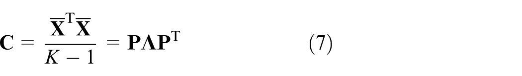
PCA-ICA process monitoring

Through selected loading vectors, PCA projects the data onto a lower-dimensional subspace that preserves the maximum variance of the original data. Sample data $x \in R^{1 \times m}$ with $m$ measured variables can be decomposed as

x = t P^{T} + ε

(1)

where $P \in R^{d \times m}$ denotes the loading matrix, $t \in R^{1 \times d}$ is the score vector, d is the number of selected principal components (PCs), and $ε \in R^{1 \times m}$ is the residual vector. PCA can preserve the dominant part of the source data if the structure of the variables of the data can be denoted as $x = Γ u + f$ ,¹⁸ where $u \in R^{n}$ is the set of source signals that contain both Gaussian and non-Gaussian components, $f \in R^{n}$ are residuals that follow a zero mean Gaussian distribution with covariance $Σ_{f}$ , $f ~ N {0, Σ_{f}}$ , and Γ is a parameter matrix. Then ICA can be applied to extract independent components (ICs) of the preserved dominant part. Given a data sample $z \in R^{d \times 1}$ , where $d$ is the number of variable, the sample can be expressed as linear combinations of $r$ ( $\leq d$ ) unknown independent components $s \in R^{r \times 1}$ added by a residual vector $ξ \in R^{d \times 1}$ , denoted as¹³

z = A s + ξ

(2)

where $A \in R^{d \times r}$ is the mixing matrix. ICA tries to find an unmixing matrix $W \in R^{r \times d}$ which makes the obtained component $\hat{s}$ as independent from each other as possible, denoted by

\hat{s} = W z

(3)

Additional details on the ICA monitoring can be found in related works.^11,13 A multivariate statistical monitoring framework is proposed, in which PCA is first employed to project the optical flow data onto the dominant subspace and then a subsequent application of ICA is employed to extract ICs from the retained PCs. The current study directly uses this PCA-ICA method to extract the independent components, and the focus is on establishing an optical flow–based motion fault detection system for monitoring the motion process.

Optical flow–based PCA-ICA fault detection

This is the first time we use unfolding optical flow feature as sample variables of PCA-ICA algorithm for motion process monitoring. The variables of the data are motion related. However, monitoring the process directly through these variables is inappropriate for three reasons. First, the motion-related variables can be correlated with each other, which can cloak the motion process behavior. Second, high dimension of the data can exceed the calculation capacity of a general computer. Third, the motion process fault can be reflected more evidently on the latent variables than on the directly variables. Considering these reasons, the present study employs the PCA-ICA method for monitoring motion process. This section displays how to unfold optical flow–based motion data to fit PCA-ICA model, how to calculate the control line of I² and SPE statistics, as well as the procedures for monitoring.

Data unfolding

The optical flow–based motion data set of a process or video is a three-way array, X(I × J × K), where I represents the number of motion points, J denotes the number of motion-related variables, and K is the number of sampling optical flow instants between each two successive frames in the video stream, which denoted as the total number of the video frames subtract one, and can also be used as time-slice index. Each optical flow item (u, v) in $G_{f}$ or $L_{f}$ corresponds to a sample point with J variable at given K. For DOF, the value of I is the number of the green points, 1080 points in Figure 1(a). Because the start position of x-axis and y-axis are the same for each frame of the video, the value of J is 4, which employs the variables just from No. 3 to No. 6 in Table 1. While for SOF, the value of I is the number of the black arrow, 25 points in Figure 1(b). The value of J is 6, which employs all motion-related variables shown in Table 1, where

d = \sqrt{{(x_{e n d} - x_{s t a r t})}^{2} + {(y_{e n d} - y_{s t a r t})}^{2}}

(4)

θ = \arctan \frac{y_{e n d} - y_{s t a r t}}{x_{e n d} - x_{s t a r t}}

(5)

Table 1.

Motion-related variables.

No. of variable	Description of motion-related variables	Symbol of variable
1	Start position at x-axis	$x_{start}$
2	Start position at y-axis	$y_{start}$
3	End position at x-axis	$x_{end}$
4	End position at y-axis	$y_{end}$
5	Displacement between $(x_{start}, y_{start})$ and $(x_{end}, y_{end})$	$d$
6	Angle between $(x_{start}, y_{start})$ and $(x_{end}, y_{end})$	$θ$

Time-wise unfolding, X is unfolded such that every slice I × J is placed along the K axis from the first time interval to the last time interval side by side. Then every slice I × J is remapped to a row vector that each row in slice I × J is concatenated from top to bottom end. A two-dimensional matrix X(K × IJ) is then constructed. Unfolding process is illustrated in Figure 2. The variation among time can be analyzed in this unfolding manner. For SOF-PCA-ICA, additional step should be taken as the row vector may not of the same length. Three methods may be employed for solving this problem: (1) align all vectors to the longest vector by filling in zero values, (2) align all vectors to the longest vector by filling in the last value of the vector, and (3) align all vectors to the shortest vector by cutting off redundant data. As the data in the vector are motion-related information, so cutting off means losing part of information and makes the model inaccurate for monitoring. Filling in the last value of the vector for aligning means adding additional nonexistent motion information which may misleading the model. Thus, we adopt align all vectors to the longest vector by filling in zero values. Before modeling, each column in X(K × IJ) needs to be scaled to zero mean and unit variance, because less important variables with large magnitudes can overshadow important variables with small magnitudes. Then, matrix $\bar{X}$ (K × IJ) is obtained.

Figure 2.

Optical flow data unfolding.

Optical flow–based PCA-ICA motion process monitoring

Reconsidering the unfolded matrix $\bar{X}$ (K × IJ) with K samples and IJ variables, PCA is performed as follows

\bar{X} = T P_{R}^{T} + E

(6)

where the loading matrix is $P_{R} (IJ \times R)$ , the score matrix is T(K × R), and the residual matrix is E(K × IJ). R is the number of principal components. $P_{R} (IJ \times R)$ can be obtained from the eigenvalue decomposition of the covariance matrix C

C = \frac{{\bar{X}}^{T} \bar{X}}{K - 1} = P Λ P^{T}

(7)

where $Λ = diag (λ_{1}, λ_{2}, \dots, λ_{IJ})$ is the eigenvalue matrix.

The eigenvalues are arranged in descending order. The principal components are ordered in the same manner as eigenvalues, such that each one describes the amount of variation in original data also in descending order. Determine R principal components, so that

\frac{\sum_{i = 1}^{R} λ_{i}}{\sum_{i = 1}^{I J} λ_{i}} \geq 90 %

(8)

P is then separated into two parts: $P_{R} (IJ \times R)$ and $P_{E} (IJ \times (IJ - R))$ . The original data can project onto $P_{R}$ and $P_{E}$ which are called principal component subspace (PCS) and residual subspace (RS), respectively

T = \bar{X} P_{R}

(9)

E = (I - P_{R} P_{R}^{T}) X

(10)

The PCS can be scaled as

Z = {Λ_{R}}^{- 1 / 2} T^{T}

(11)

where $Λ_{R} = diag (λ_{1}, λ_{2}, \dots, λ_{R})$ , $Z \in R^{R \times K}$ . Based on selected PCs, ICA can be applied to extract the independent components. The ICs $S \in R^{R \times K}$ can be obtained as

S = WZ

(12)

where $W \in R^{R \times R}$ is the unmixing matrix. When a fault occurs in a motion process, the fault can cause certain changes or deviations. The $s_{i} \in R^{R \times 1}$ is the ith column of S, and the I² statistic $I_{i}^{2} = s_{i}^{T} s_{i}$ is constructed to measure the variation directly along each time index. A non-parametric, KDE method, is used to estimate distributions of ICs, because the ICs do not usually follow Gaussian distribution assumption. Using KDE method, the probability density function of random variable $x$ is given by the following formula

f (x) = \frac{1}{nh} \sum_{i = 1}^{n} k (\frac{x - x_{i}}{h})

(13)

where $x_{i}$ is the ith sample of random variable $x$ , $n$ is the number of samples, $h$ is the bandwidth parameter, and $k (\cdot)$ denotes the kernel function which follows that

\int_{- \infty}^{\infty} k (x) d x = 1, k (x) \geq 0

(14)

In practice, the bandwidth parameter $h$ has a crucial effect on the performance of KDE. Many criterions such as least squares cross-validation and biased cross-validation were developed to select the optimal value of parameter $h$ . The optimal value of parameter $h$ given in Mugdadi and Ahmad²⁹ which determined by the least square cross-validation method is

h = 1.06 Σ n^{- 0.2}

(15)

where $Σ$ is the standard deviation and $n$ is the number of samples. Dehnad³⁰ shows more details regarding KDE technique. The SPE statistic can be constructed to monitor the PCA RS as

SPE = e e^{T}, e = \bar{x} - \bar{x} P_{R} {P_{R}}^{T}

(16)

where $\bar{x} (1 \times IJ)$ is the monitored sample, which has been unfolded on time-wise and each column of which is normalized, and e indicates the residuals at time k with the IJ variables. For SOF-PCA, the IJ in $\bar{x} (1 \times IJ)$ , say IJ′, may be different from IJ in $P_{R} (IJ \times R)$ , and we need to match IJ′ and IJ to the same size for calculating T², I², and SPE. If IJ′ is larger than IJ, then use the first IJ column of $\bar{x} (1 \times IJ')$ . If IJ′ is smaller than IJ, then fill in zero values to align the column of $\bar{x} (1 \times IJ')$ to $\bar{x} (1 \times IJ)$ . For IJ is the column size of the longest vector in SOF-PCA-ICA model, in most of time IJ′ is smaller than IJ. Proper control limits of SPE are defined to determine whether the motion process is under normal conditions as follows

SP E_{β} = g χ_{h, β}^{2}, g = \frac{v}{2 μ}, h = \frac{2 μ^{2}}{v}

(17)

where $F_{R, N - R, β}$ is an F distribution with $R$ and $N - R$ degrees of freedom under confidence limit $β$ and $μ$ and $v$ are the estimated mean and variance, respectively, of the squared prediction error from the modeling data.

The optical flow–based PCA-ICA approach for online process monitoring is illustrated in Figure 3, and its detailed step-by-step procedure is given in the following:

Off-line modeling

1. Extract optical flow and unfold X(I × J × K) to X(K × IJ).

2. Obtain $\bar{X}$ by normalizing the data X in each column.

3. Determine R, P_R, and calculate the control limit SPE_line of SPE.

4. Whiten the data in PCS to get unmixing matrix W and ICs.

5. Calculate I² statistic.

6. Using KDE to estimate the control limit I²_line of I².

Online monitoring

1. Normalize the test sample x, extracted optical flow data between k – 1 and k frames of test video, using the same data of the model.

2. Project the data into PCS. Calculate SPE in RS.

3. Do ICA in PCS to get ICs.

4. Calculate I² statistic.

5. Monitor whether the value of I² exceeds the I²_line and SPE exceeds the SPE_line.

Figure 3.

Flow chart of process monitoring.

Case study

In this section, the proposed DOF-PCA-ICA and SOF-PCA-ICA motion process monitoring approaches are evaluated through the RABMS. Robotic-arm-based system is widely used in industry, and the marking system which is used in steel enterprises is an example of this kind. Steel enterprises need to mark important parameters, the mintmark, size, batch number, date, and other information, to meet the standard management rules. Traditionally, the marking work is done by human workers. Because of the bad working conditions, high temperate, hazardous, and noxious substances, and repetitive work for a long time in fast speed, it is unavoidable for human workers to mark occasionally the wrong label on the products. So, RABMS shown in Figure 4 is designed for replacing human labor to enhancing marking efficiency with high quality. As can be seen in Figure 4, the RABMS holds a spray gun at its robotic arm’s end and the spay gun can be freely moved by its arm to any position along the half arc surface of the coil toward the robot to mark the information. The coil is taken by walking beam soon after being bundled; therefore, it is of high temperature about 300°C. During the 1-min stay, the RABMS will use radius measure end of the spray gun to touch three different spots of the coil surface to calculate the radius of the coil if radius meets the demand and then the spray end will be rotated to mark the information; otherwise, the robot will refuse to mark and get back to its rest room where there is a partition diving off the hot coil. Finally, the coil will be moved to another area by the walking beam waiting for electromagnet crane to carry away to the stacking area.

Figure 4.

Robotic-arm-based marking system

We capture a video stream of 1 min and 12 s, which contains 1727 frames whose size is 624 × 416 pixels to do a model of normal motion of the RABMS. If we use DOF-PCA-ICA model, and both horizontal and vertical interval steps are 16 pixels, we get X(1080 × 4 × 1727), then after unfolding and normalization, we get $\bar{X}$ (1727 × 4320). If we use SOF-PCA-ICA model with the same video stream, we get X(261 × 6 × 1727), which means 261 is the largest number of the motion points detected among all model video frames; then after unfolding and normalization, we get $\bar{X}$ (1727 × 1566). The time of the test video stream is 3 min and 30 s, which contains 5037 frames and several faults listed in Table 2. Data of test sample are $\bar{x} (1 \times 4320)$ if DOF-PCA-ICA model is used. While if SOF-PCA-ICA model is used, the data of test sample are $\bar{x} (1 \times (6 \times n))$ , which means the size of test sample is dependent on the value of the number of detected motion points n in current test video frame, and for different frames, the number of n may be different. The corresponding ways for solving this problem are illustrated in section “Optical flow–based PCA-ICA motion process monitoring.” All the videos used in our experiments are captured by a fixed Nikon camera.

Table 2.

Fault descriptions of RABMS.

Fault description	Frames
Fault 1: human moves in dangerous area which is forbidden for safety reason	2400–3300
Fault 2: vibration of the spray gun	3450–3470

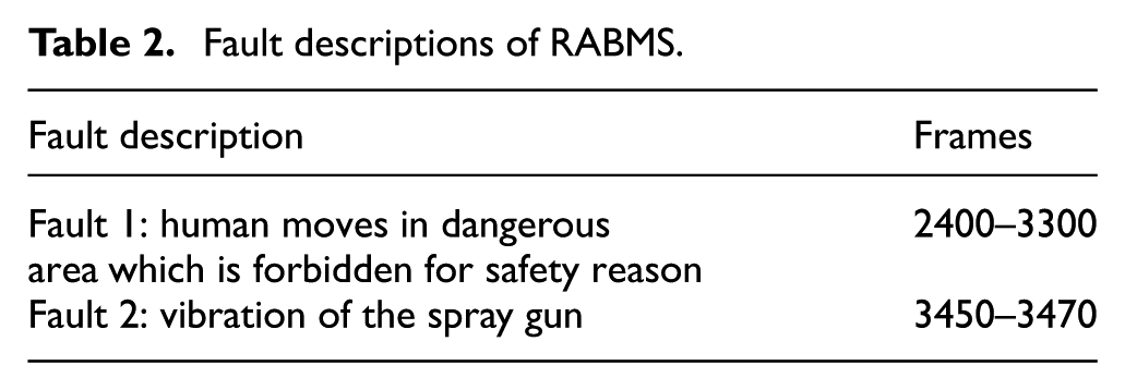
Effects of the faults are analyzed as follows. Human workers move in the area around the robot which may be dangerous for safety reasons. Fault 2 is quality related that may cause flaw mark or even wrong mark due to the motion data that do not in accordance with the normal model motion data. The total number of fault frame is 922.

Both the DOF-PCA-ICA and SOF-PCA-ICA are applied to monitor the motion process, and the performance of these methods is compared. We do the PCA algorithm to normal model to extract principle component, and through the sample points we get each component’s contribution according to formula (8). Therefore, we select the first 769 and 10 variables for DOF-PCA-ICA and SOF-PCA-ICA as our principal components, and the contributions of the selection over that of the total are above 90%. The corresponding 769 and 10 columns of P for DOF-PCA-ICA and SOF-PCA-ICA are persevered for forming $P_{R}$ matrix, respectively, and their PCS can also be derived by formulas (9) and (10). The normal probability plot of the ninth score (t₉) vector calculated by applying PCA to the normal model data in Figure 5 makes it clear that the values of t₉ do not follow a Gaussian distribution.

Figure 5.

Normality check of ninth score obtained from PCA.

FastICA is performed after projecting the data onto the PCS, 769 ICs for DOF-PCA-ICA and 10 ICs for SOF-PCA-ICA are used for calculating I² statistic. All the 1727 frames of model video are used for estimating the normal distribution of I² statistic. The I² is within [39,622] for DOF-PCA-ICA and [0,7] for SOF-PCA-ICA as shown in Figures 6 and 7.

Figure 6.

Distribution of I² using DOF-PCA-ICA.

Figure 7.

Distribution of I² using SOF-PCA-ICA model.

Interval [39,622] is divided into 100 subintervals, and the frequency ratio of I² within each subinterval is derived. Then, KDE is used for fitting these discrete points for DOF-PCA-ICA in Figure 8. The same is done to interval [0,7]. The frequency ratio of I² within each subinterval and the KDE for fitting these discrete points for SOF-PCA-ICA is shown in Figure 9. Finally, the I²_line of I² statistic with 99% confidence is 441.22 and 0.067 for DOF-PCA-ICA and SOF-PCA-ICA monitoring, respectively.

Figure 8.

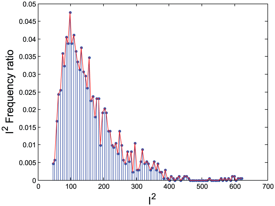
Estimation of I² control limit using DOF-PCA-ICA.

Figure 9.

Estimation of I² control limit using SOF-PCA-ICA model.

Figures 10 and 11 demonstrate the monitoring performance for faults in Table 2 through I² statistic using DOF-PCA-ICA method. As can be seen in Figure 10, when the worker moves fast in dangerous area, the value of I² statistic is large, for example, frames 2414–2358, frames 2737–2957, and frames 3155–3280. Similarly, when the worker moves slowly in dangerous area, the value of I² statistic is small, for example, frames 2538–2737 and frames 2967–3155. The performance for the same faults in Table 2 through I² statistic using SOF-PCA-ICA method is shown in Figure 12. It obtains similar results as DOF-PCA-ICA model. But some points of I² statistic value is zero, because some minor movement cannot be detected by the SOF extraction.

Figure 10.

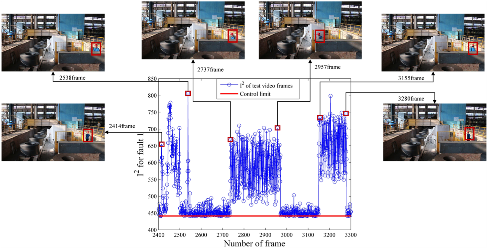
Plot of I² using DOF-PCA-ICA for monitoring fault 1.

Figure 11.

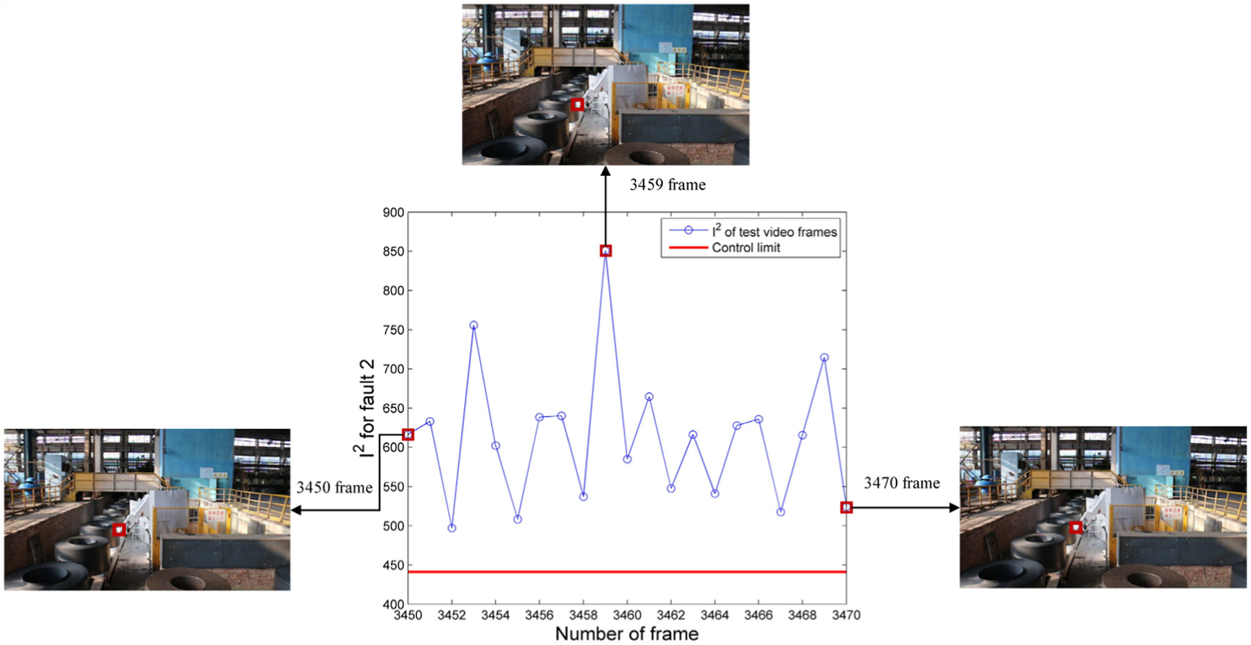
Plot of I² using DOF-PCA-ICA for monitoring fault 2.

Figure 12.

Plot of I² using SOF-PCA-ICA for monitoring.

The fault detection rates of the proposed DOF-PCA-ICA and SOF-PCA-ICA methods are listed in Table 3. To make a contrast with the PCA algorithm, the detection results by T² and SPE statistics are also listed in Table 3. From Table 3, the DOF-PCA-ICA method using I² statistic has the best performance. While the SOF-PCA-ICA method using I² statistic, DOF-ICA and SOF-ICA also have well enough performance. Although the DOF-ICA and SOF-ICA perform well enough on detection rate and false alarm rate, the process time takes far more than the proposed method, in case study more than 48 h for processing DOF-ICA model and 5 h for SOF-ICA model. Therefore, it may be impossible for applying the DOF-ICA and SOF-ICA in real-time application.

Table 3.

Comparison results of given faults.

Fault no.	Detection rate										False alarm rate
	DOF-PCA-ICA		SOF-PCA-ICA		DOF-ICA	SOF-ICA	DOF-PCA		SOF-PCA		DOF-PCA-ICA		SOF-PCA-ICA		DOF-ICA	SOF-ICA	DOF-PCA		SOF-PCA
	I ²	SPE	I ²	SPE	I ²	I ²	T ²	SPE	T ²	SPE	I ²	SPE	I ²	SPE	I ²	I ²	T ²	SPE	T ²	SPE
1	92.74	5.33	87.46	46.06	91.12	90.01	3.77	5.33	50.94	46.06	8.73	16.88	13.7	22.55	4.85	5.45	27.18	25.85	21.15	24.27
2	100	66.67	71.43	33.33	90.48	85.71	61.9	66.67	57.14	33.33	5.88	8.24	7.06	16.47	7.06	7.65	10.59	8.24	11.18	12.35

DOF: dense optical flow; PCA: principal component analysis; ICA: independent component analysis; SOF: sparse optical flow.

Significance of bold values are for highlighting the results compared to other methods.

The performance of data size and process time is of great value in real application, and the results are shown in Table 4. Data size means the occupied memory space on hard disk. Process time means consumed time for processing the data. The performance of data size and process time for the proposed methods is given in Table 4.

Table 4.

Comparison results of performance.

	Model video	DOF model	SOF model	Test video	DOF test	SOF test
Data size	104 MB	28.4 MB	363 KB	131 MB	17 KB	0.06 KB
Process time	71 s	209 s	1.76 s	90 s	2.6 ms	0.33 ms

From Table 4, DOF-PCA-ICA method needs more space and consumes more time for processing both model and test data than SOF-PCA-ICA method. The reason for DOF-PCA-ICA’s good performance for fault detection is that it contains more detail information than SOF-PCA-ICA. On the other hand, SOF-PCA-ICA also has the ability for detecting all faults in Table 2 with fewer space and faster speed. All in all, it depends on your need to choose which method to use for motion monitoring.

Conclusion

In this article, for the first time, optical flow feature and PCA-ICA algorithm are combined for developing motion process monitoring algorithms. Two kinds of optical flow, DOF and SOF, are employed as the samples of motion-related variables for forming models of DOF-PCA-ICA and SOF-PCA-ICA. Based on the model, the corresponding motion process monitoring scheme is proposed. The proposed monitoring approaches are applied to monitor robotic-arm-based spray marking system. The case study results demonstrate that both DOF-PCA-ICA and SOF-PCA-ICA can detect the faults designed in Table 2. Compared to SOF-PCA-ICA, the DOF-PCA-ICA model is more accurate but consumes more time and memory space. So, when accuracy is most important index, we should choose DOF-PCA-ICA model. Otherwise, when speed is most important index, we should choose SOF-PCA-ICA model.

Footnotes

Handling Editor: Kuei Hu Chang

Declaration of conflicting interests

The author(s) declared no potential conflicts of interest with respect to the research, authorship, and/or publication of this article.

Funding

The author(s) disclosed receipt of the following financial support for the research, authorship, and/or publication of this article: The work is supported by NSF in China (61325015 and 61733003).

References

Chiang

Russell

Braatz

. Fault detection and diagnosis in industrial systems. London: Springer Verlag, 2001.

Ding

. Data-driven design of monitoring and diagnosis systems for dynamic processes: a review of subspace technique based schemes and some recent results. J Process Contr 2013; 24: 431–449.

Fan

Zhang

. Intelligent fault isolation of nonlinear processes with expert guidance. Adv Mech Eng 2017; 9: 1–13.

Song

Gao

. Review of recent research on data-based process monitoring. Ind Eng Chem Res 2013; 52: 3543–3562.

Qin

. Statistical process monitoring: basics and beyond. J Chemometr 2003; 17: 480–502.

Yin

Ding

Xie

et al . A review on basic data-driven approaches for industrial process monitoring. IEEE T Ind Electron 2014; 61: 6418–6428.

Yata

Aoshima

. PCA consistency for non-Gaussian data in high dimension, low sample size context. Comm Stat Theor Meth 2009; 38: 2634–2652.

Lou

Shen

Wang

. Preliminary-summation-based principal component analysis for non-Gaussian processes. Chemometr Intell Lab 2015; 146: 270–289.

Huang

Yan

. Gaussian and non-Gaussian double subspace statistical process monitoring based on PCA and ICA. Ind Eng Chem Res 2015; 54: 1015–1027.

10.

Jiang

Yan

. PCA-ICA integrated with Bayesian method for non-Gaussian fault diagnosis. Ind Eng Chem Res 2016; 55: 4979–4986.

11.

Hyvärinen

Oja

. Independent component analysis: algorithms and applications. Neural Networks 2000; 13: 411–430.

12.

Lee

Yoo

Lee

. Statistical process monitoring with independent component analysis. J Process Contr 2004; 14: 467–485.

13.

Kano

Tanaka

Hasebe

et al . Monitoring independent components for fault detection. AIChE J 2003; 49: 969–976.

14.

Learned-Miller

Fisher III

. ICA using spacings estimates of entropy. J Mach Learn Res 2010; 4: 1271–1295.

15.

Chang

Lee

Vanrolleghem

et al . On-line monitoring of batch processes using multiway independent component analysis. Chemometr Intell Lab 2004; 71: 151–163.

16.

Lee

Yoo

Lee

. Statistical process monitoring with independent component analysis. J Process Contr 2004; 14: 467–485.

17.

Zhang

Qin

. Fault detection of nonlinear processes using multiway Kernel independent component analysis. Ind Eng Chem Res 2007; 46: 7780–7787.

18.

Liu

Xie

Kruger

et al . Statistical-based monitoring of multivariate non-Gaussian systems. AIChE J 2008; 54: 2379–2391.

19.

Berg

Bondesson

Low

et al . A combined on-line PCA-ICA algorithm for blind source separation. In: Asia-Pacific conference on communications, Perth, WA, Australia, 5 October 2005, pp.969–972. New York: IEEE.

20.

Megahed

Woodalland

Camelio

. A review and perspective on control charting with image data. J Qual Technol 2011; 43: 83–98.

21.

Wang

Tsung

. Using profile monitoring techniques for a data rich environment with huge sample size. Qual Reliab Eng Int 2005; 21: 677–688.

22.

Megahed Wells

FMLJ

Camelio

Woodall

. A spatiotemporal method for the monitoring of image data. Qual Reliab Eng Int 2012; 28: 967–980.

23.

Duchesne

Liuand MacGregor

. Multivariate image analysis in the process industries: a review. Chemometr Intell Lab 2012; 117: 116–128.

24.

Barron

Fleet

Beauchemin

. Performance of optical flow techniques. Int J Comput Vision 1994; 12: 43–77.

25.

Bouguet

. Pyramidal implementation of the Lucas Kanade feature tracker description of the algorithm. Intel Corp Microprocessor Res Lab Tech Rep 2000; 22: 363–381.

26.

Farnebäck

. Two-frame motion estimation based on polynomial expansion. Image Anal 2009; 2749: 363–370.

27.

Alvarez

Deriche

Papadopoulo

et al . Symmetrical dense optical flow estimation with occlusion detection. Int J Comput Vision 2002; 75: 371–385.

28.

Senst

Eiselein

Sikora

. II-LK—a real-time implementation for sparse optical flow. In: Campilho

Kamel

(eds) Image analysis and recognition. Berlin: Springer, 2010, pp.240–249.

29.

Mugdadi

Ahmad

. A bandwidth selection for kernel density estimation of functions of random variables. Comput Stat Data An 2004; 47: 49–62.

30.

Dehnad

. Density estimation for statistics and data analysis. London: Chapman & Hall, 1986, pp.296–297.