Analytical modelling of flame transfer functions for technically premixed flames

Abstract

The linear response to harmonic acoustic excitation of the total heat release rate in technically premixed flames (Flame Transfer Function, FTF) is studied in case of an ideal swirl burner. The analysis is based on the linearization of the production rate for the mean reaction progress variable modelled with a turbulent flame speed closure. Three main components of the FTF are identified which are generated by: I) direct fluctuations in the fuel mixture fraction (formation enthalpy contribution), II) direct fluctuations in the turbulent flame speed and III) flame surface area fluctuations driven by velocity and turbulent flame speed fluctuations. The velocity fluctuation is separated into an irrotational acoustic displacement and a rotational convective component. The effect of the rotational velocity component on the FTF is modelled here in a semi-empirical way, related to swirl number fluctuations at the flame base due to the phase shift between convected tangential velocity fluctuations and acoustically propagating axial velocity fluctuations. It is finally shown that fuel mixture fraction fluctuations can be generated not only by air mass flow rate fluctuations but also by fuel flow rate fluctuations which depend upon the air side impedance at the fuel injection location. It is shown that this impedance changes with the geometry of the plenum placed upstream the burner affecting in this way also the FTF.

Keywords

Lean Premixed Combustion thermoacoustics flame Dynamics

Introduction

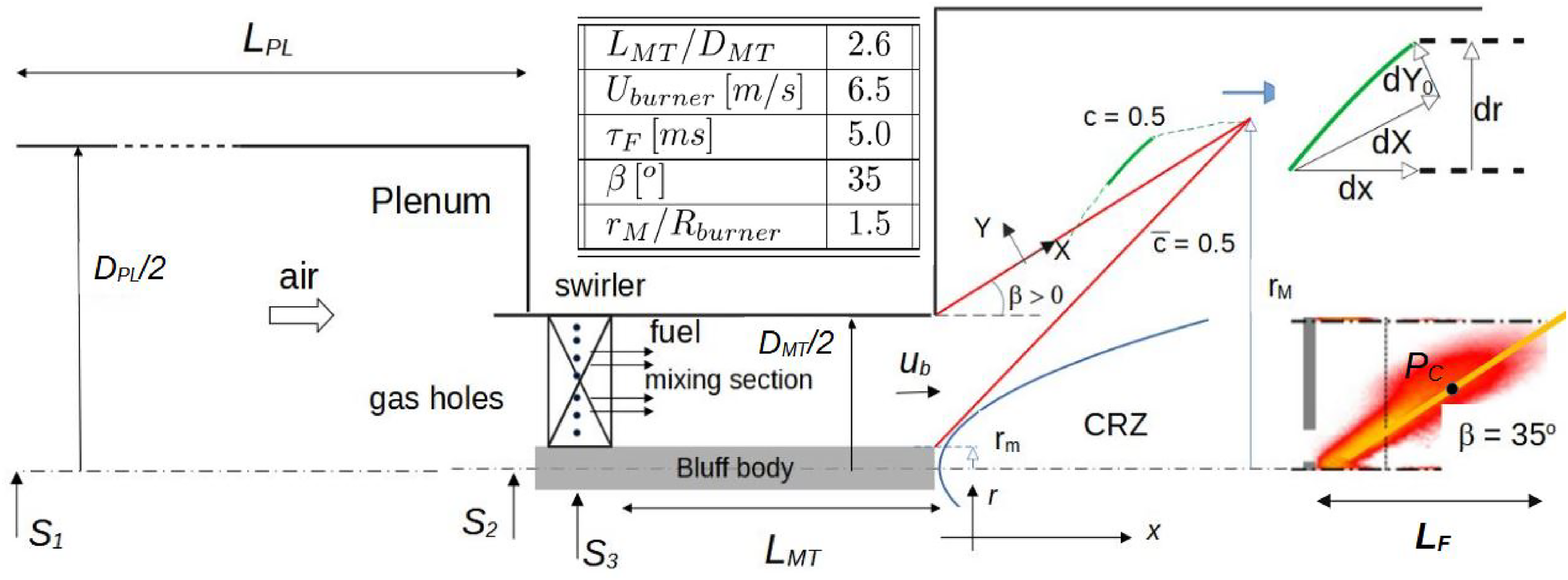
Lean premixed combustion has been for long time the solution for the reduction of NOx emissions from industrial gas turbines. Effective stabilization of turbulent lean premixed flames in industrial burners is usually obtained triggering the phenomenon of vortex breakdown.¹This phenomenon consists in the formation of a central recirculation zone (CRZ) acting as an aerodynamic flameholder,² when sufficiently high swirl is given to the flow of reactants. Swirl stabilized lean premixed flames can cause thermoacoustic instabilities via the coupling between the acoustic field, the unsteady heat release and the swirl characteristics of the flow. Thermo-acoustic instabilities are often studied via a low-order network approach, see for example,³ where the combustion system is decomposed in a network of elements. Each element is mathematically characterized by a transfer matrix which relates acoustic velocity and pressure between output and input ports. One important and complex element of the thermoacoustic network is the flame. In case of low Mach number flows and acoustically compact flames, the main element of the flame transfer matrix is given by the relation between the acoustic velocity downstream to the acoustic velocity upstream the flame (often indicated as the $T_{22}$ element). This element depends directly from the Flame Transfer Function, FTF, i.e. the response of total unsteady heat release (relative to the mean value) with respect to the fluctuation of acoustic displacement velocity (relative to the mean convection velocity) at the base of the flame, i.e. $(\hat{\dot{Q}} / \bar{\dot{Q}}) / ({\hat{u}}_{b} / {\bar{u}}_{b})$ , see Figure 1.

Figure 1.

Schematic of inner and outer axisymmetric-symmetric M flame (only top half shown) stabilized by the vortex breakdown mechanism.

The FTF can be determined experimentally or numerically for example via Computational Fluid Dynamics (CFD). A widely used experimental approach,⁴ consists in exciting the acoustic field via loudspeakers at discrete values of the frequency and measuring acoustic waves via microphones placed upstream and downstream the flame. In case of CFD, the excitation is instead usually applied at the inlet boundary as a velocity or mass flow rate perturbation around the mean value and the total unsteady heat release determined at each time step of the simulation. In order to keep the computational effort+ within acceptable limits, the excitation is typically applied as a broadband signal containing energy in the frequency range of interest. The FTF is therefore determined⁵ using techniques for the system identification of dynamic systems.

Under some simplifying assumptions, the problem can be studied also analytically based on the G-equation^6–10 formalism where the flame is approximated as an infinitesimally thin surface propagating with a given consumption speed. Given the complexity of the physical mechanisms governing swirl stabilized flames, the analytical approach cannot be obviously expected to be as complete as CFD where most of the involved physics is numerically resolved. The analytical formulation allows however a relatively simple separation of the FTF into contributions driven by different physical mechanisms while the CFD approach works more in a ’black box’ fashion. For this reason the analytical approach is also adopted here with the scope of an insight into the mechanisms driving the flame response to the acoustic perturbation. The novelty of the present work consists in placing particular attention on the effect of the impedance, i.e. the ratio between acoustic pressure and velocity in the air flow, at the position of fuel injection. This impedance has impact on the importance of the contribution to the FTF driven by fuel mass flow rate fluctuations with respect to the contribution driven directly by air velocity fluctuations. The FTF can therefore loose its uniqueness given the dependency of such impedance, for example, from the geometry of the plenum placed upstream the burner.

The work is presented below considering first the identification of several different contributions to the linearized total heat release. A qualitative validation and tuning of the model parameters is subsequently carried out with FTF experimental data for fully premixed turbulent flames. Finally, the effect of air impedance on the FTF is evaluated for two values of the length of the plenum placed upstream the burner and different values of the equivalence ratio.

Modelling

The Flame Transfer Function is given by:

F = \frac{\hat{\dot{Q}} / \bar{\dot{Q}}}{{\hat{u}}_{b} / {\bar{u}}_{b}}, \dot{Q} = \int_{V} \dot{q} d V

(1)

where

\dot{q}

and

\dot{Q}

represent respectively the local and total rates of heat release,

u_{b}

the velocity at the flame base and

\hat{ϕ} (f_{q})

is complex valued, representing the harmonic response of the generic variable

ϕ

at frequency

f_{q}

, i.e.

ϕ (t) = ℜ [\hat{ϕ} \exp (j ω t)]

with

ω = 2 π f_{q}

The analytical modelling of the FTF considered here is based on the source of the mean reaction progress variable used in the modelling of turbulent premixed flames. This source can be expressed in terms of the turbulent burning rate $U_{t}$ , i.e. the volumetric consumption of reactants for unit of time and unit of mean flame area¹¹, as:

{\dot{q}}_{c} = ρ_{u} U_{t} ∣ \nabla c ∣

(2)

with

U_{t} = A_{T F C} u^{'} D a^{1 / 4} = A_{T F C} u^{' 3 / 4} l_{t}^{1 / 4} λ^{- 1 / 4} s_{L}^{1 / 2}

(3)

where

A_{T F C}

is a constant of the order of unity and where the usual Favre averaging notation has been omitted.

Under lean conditions, the local heat release rate $\dot{q}$ is obtained from the source term given by relation (2) (representing the rate of reactants mass consumption) times the fuel mixture fraction $f$ times the calorific value of the fuel $H_{c}$ :

\dot{q} = ρ_{u} f H_{c} U_{t} ∣ \nabla c ∣

(4)

The linearization of the total heat release rate is considered in the next section.

Linearization

Assuming small perturbations, the analysis is carried out with the linearized form of equation (2) and relation (4), under the condition of axial symmetry. For an infinitesimal flame element of length $d l_{F}$ and area $d A_{F}$ (taken on the iso-surface $c = 0.5$ , see Figure 1), integrating relation (4) orthogonally to the flame yields:

{\dot{q}}_{A} = ρ_{u} f H_{c} U_{t} d A_{F}

(5)

whose linearization gives (harmonic fluctuations assumed):

{\hat{\dot{q}}}_{A} = ρ_{u} H_{c} (\hat{f} \bar{U_{t}} d {\bar{A}}_{F} + \bar{f} {\hat{U}}_{t} d {\bar{A}}_{F} + \bar{f} \bar{U_{t}} d {\hat{A}}_{F})

(6)

where

d {\hat{A}}_{F}

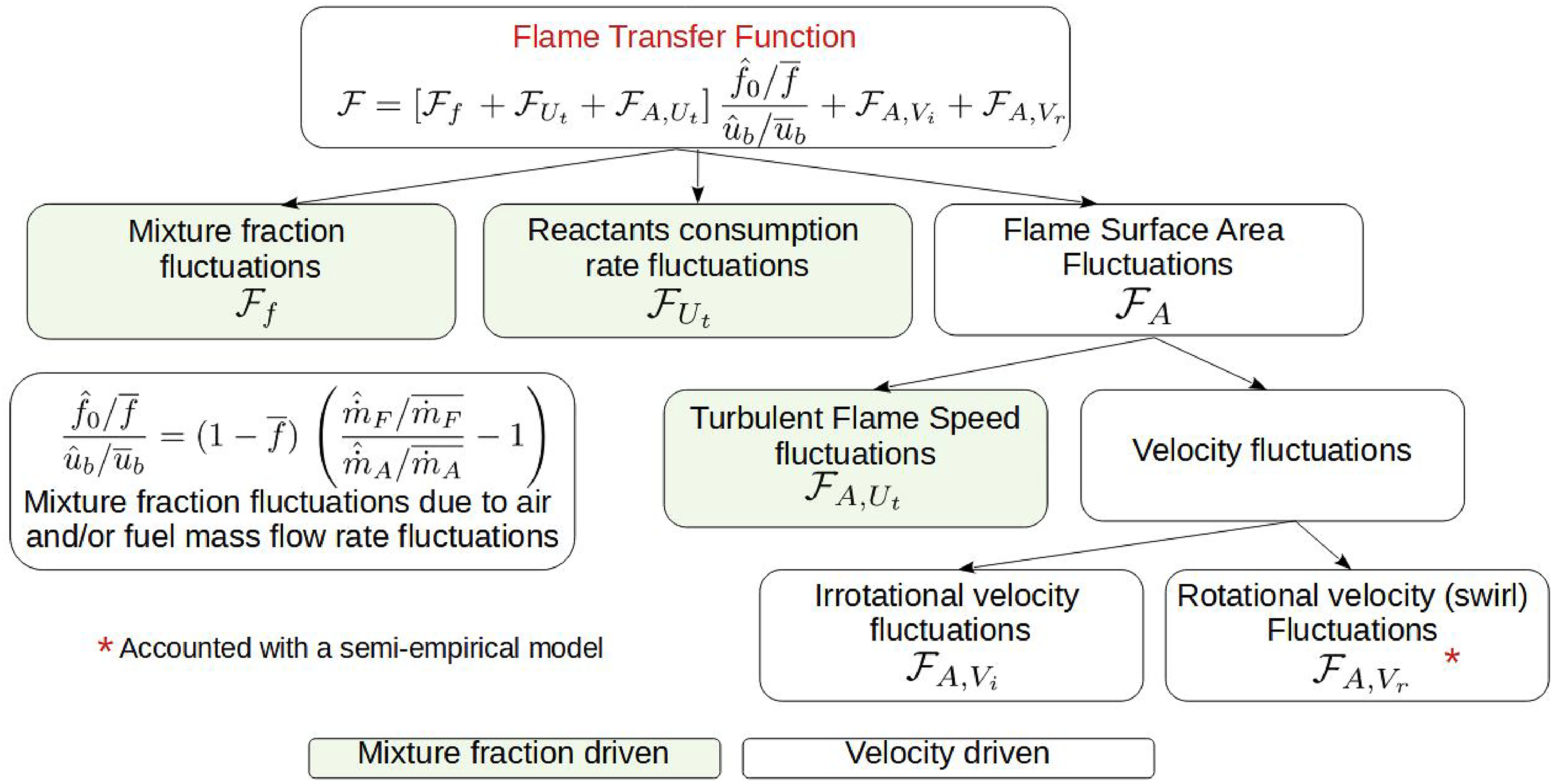
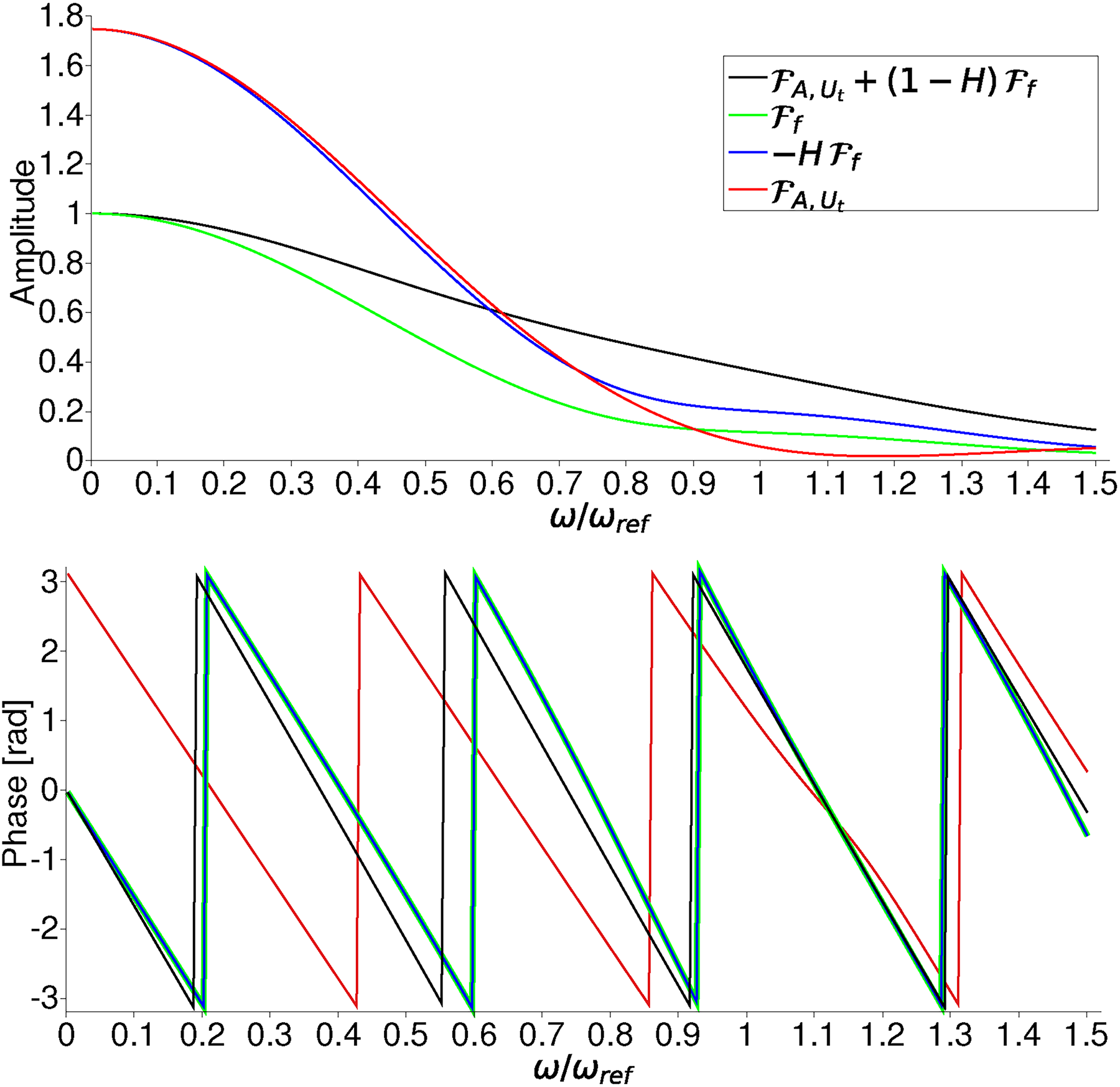
represents the local deviation of surface area from the mean value

d {\bar{A}}_{F}

for the infinitesimal flame element and where the density of unburnt reactants

ρ_{u}

is considered constant. Before progressing further it is worth discussing relation (6) on the basis of Figure 2 showing how the FTF is decomposed below into different contributions. Three different main contributions to unsteady heat release can be identified from relation (6): due to direct fuel mixture fraction, turbulent flame speed and flame surface fluctuations. It will be shown below that flame surface area fluctuations are generated by two distinct mechanism: due to turbulent flame speed and velocity fluctuations. Additionally, the velocity driven part of the flame surface area fluctuations can be decomposed into two more contributions, related to the irrotational and rotational components of the velocity field. Finally, fluctuations in turbulent flame speed are due mostly to fuel mixture fraction fluctuations which in turn depend on fluctuations in air and fuel mass flow rate at the location of fuel injection.

Figure 2.

Summary of FTF decomposition into different types of contributions

Assuming that mean quantities are all uniform, the fluctuation of total heat release with respect to its mean value is given by:

\frac{\hat{\dot{Q}}}{\bar{\dot{Q}}} = \frac{1}{{\bar{A}}_{F}} [\frac{1}{\bar{f}} \int_{{\bar{A}}_{F}} \hat{f} d {\bar{A}}_{F} + \frac{1}{{\bar{U}}_{t}} \int_{{\bar{A}}_{F}} {\hat{U}}_{t} d {\bar{A}}_{F} + {\hat{A}}_{F}]

(7)

Three different components of

\hat{\dot{Q}} / \bar{\dot{Q}}

can be identified again in relation (7): the first directly related to fuel mixture fraction fluctuations and representing fluctuation in reactants formation enthalpy, the second directly related to fluctuations in the turbulent burning rate and the third to flame surface area fluctuations.

The flame surface area fluctuation can be worked out in terms of the deviation $Y_{0}$ of the $c = 0.5$ iso-surface from the mean $\bar{c} = 0.5$ iso-surface in a frame of reference $X, Y$ attached to the mean flame with $Y$ oriented from the reactants to the products. The following relations are obtained from the schematic of Figure 1 in this frame of reference:

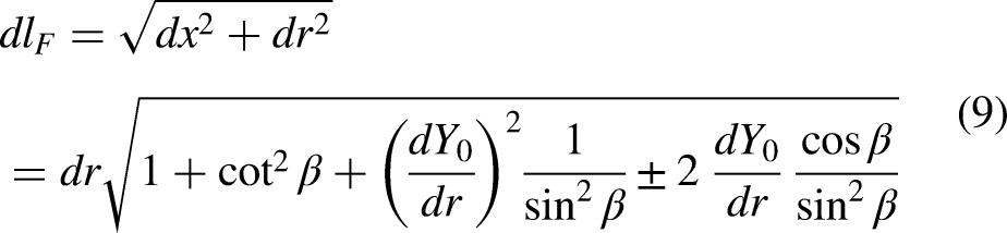
{\begin{matrix} d x = d X \cos β \pm d Y_{0} \sin β \\ d r = d X \sin β \mp d Y_{0} \cos β \end{matrix} \to d x = d r \cot β \pm \frac{d Y_{0}}{\sin β}

(8)

where the upper and bottom signs apply respectively to the inner and the outer flames and where

β

represents the angle between the flame and the central axis. The length of the flame element is given by:

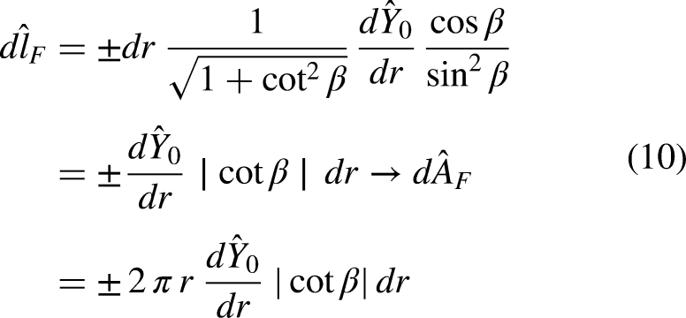
\begin{aligned} d l_{F} = \sqrt{d x^{2} + d r^{2}} \\ = d r \sqrt{1 + \cot^{2} β + {(\frac{d Y_{0}}{d r})}^{2} \frac{1}{\sin^{2} β} \pm 2 \frac{d Y_{0}}{d r} \frac{\cos β}{\sin^{2} β}} \end{aligned}

(9)

whose linearization in case of harmonic fluctuations yields:

\begin{aligned} d {\hat{l}}_{F} & = \pm d r \frac{1}{\sqrt{1 + \cot^{2} β}} \frac{d {\hat{Y}}_{0}}{d r} \frac{\cos β}{\sin^{2} β} \\ = \pm \frac{d {\hat{Y}}_{0}}{d r} ∣ \cot β ∣ d r \to d {\hat{A}}_{F} \\ = \pm 2 π r \frac{d {\hat{Y}}_{0}}{d r} | \cot β | d r \end{aligned}

(10)

In the cylindrical coordinate system the following non-dimensional parameters are also introduced:

\begin{aligned} η & = \frac{r - r_{m}}{r_{M} - r_{m}}, τ_{F} = \frac{r_{M} - r_{m}}{\sin β \bar{U}} \\ X - X_{i n} & = \frac{r - r_{m}}{\sin β} = \frac{η}{\sin β} (r_{M} - r_{m}), \\ Ω & = ω τ_{F} \to ω \frac{X - X_{i n}}{\bar{U}} = Ω η \end{aligned}

(11)

where

\bar{U}

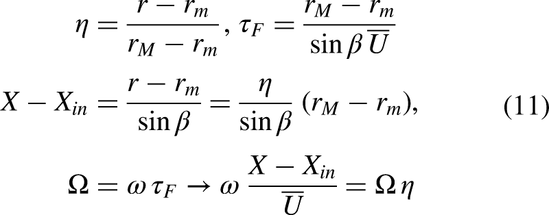
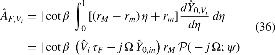
is the projection of the mean flow velocity along the mean flame,

X_{i n}

is the location of the flame anchoring point and

r_{m}, r_{M}

radiuses respectively at the base and the end of the flame. Using relations (11) into (10) and integrating over the whole mean flame, leads to the following expression for the total fluctuating flame surface area (given for one radiant):

{\hat{A}}_{F} = \int_{0}^{1} [(r_{M} - r_{m}) η + r_{m}] ∣ \cot β ∣ \frac{d {\hat{Y}}_{0}}{d η} d η

(12)

The deviation

{\hat{Y}}_{0}

is usually determined from the linearization of the

G

-equation, where the flame is assumed as an infinitesimal propagating thin boundary. In this work we have linearized directly the rate of the reaction progress variable (2). In case of turbulent flows, where the flame brush thickness is finite and growing due to turbulent dispersion, this rate is more appropriate than the rate used in the classic

G

-formalism for infinitesimally thin flames. This linearization (not shown here) leads to the result below:

j ω {\hat{Y}}_{0} + \bar{U} \frac{d {\hat{Y}}_{0}}{d X} = \hat{V} - {\hat{U}}_{t}

(13)

where

\hat{V}

{\hat{U}}_{t}

are harmonic fluctuations respectively of the flow velocity orthogonal to the mean flame and of the turbulent burning rate. The solution of this equation can be found multiplying both sides by

\exp (j ω X / \bar{U})

which gives:

\frac{d}{d X} [{\hat{Y}}_{0} \exp (j ω \frac{X}{\bar{U}})] = \frac{\hat{V} - {\hat{U}}_{t}}{\bar{U}} \exp (j ω \frac{X}{\bar{U}})

(14)

Integrating this equation along the mean flame starting at

X = X_{i n}

gives:

\begin{aligned} {\hat{Y}}_{0} (X) & = {\hat{Y}}_{0, i n} \exp (- j ω \frac{X - X_{i n}}{\bar{U}}) \\ + \exp (- j ω \frac{X}{\bar{U}}) \int_{X_{i n}}^{X} \frac{\hat{V} - {\hat{U}}_{t}}{\bar{U}} \exp (j ω \frac{ξ}{\bar{U}}) d ξ \end{aligned}

(15)

Under the assumption of uniform

\bar{U}

, using the non-dimensional parameters (11), this last equation can be cast as:

\begin{aligned} {\hat{Y}}_{0} (η) = \exp (- j Ω η) \\ \times ({\hat{Y}}_{0, i n} + τ_{F} \int_{0}^{η} (\hat{V} - {\hat{U}}_{t}) \exp (j Ω ξ) d ξ) \end{aligned}

(16)

which will be used below to work out the contribution of flame surface area fluctuations to the total FTF.

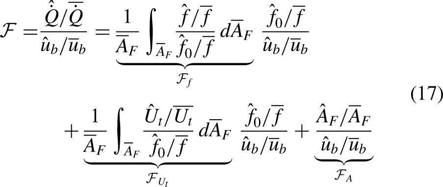
The FTF $F$ is obtained dividing relation (7) by ${\hat{u}}_{b} / {\bar{u}}_{b}$ , see relation (1):

\begin{aligned} F = & \frac{\hat{\dot{Q}} / \bar{\dot{Q}}}{{\hat{u}}_{b} / {\bar{u}}_{b}} = \underset{F_{f}}{\underset{⏟}{\frac{1}{{\bar{A}}_{F}} \int_{{\bar{A}}_{F}} \frac{\hat{f} / \bar{f}}{{\hat{f}}_{0} / \bar{f}} d {\bar{A}}_{F}}} \frac{{\hat{f}}_{0} / \bar{f}}{{\hat{u}}_{b} / {\bar{u}}_{b}} \\ + \underset{F_{U_{t}}}{\underset{⏟}{\frac{1}{{\bar{A}}_{F}} \int_{{\bar{A}}_{F}} \frac{{\hat{U}}_{t} / \bar{U_{t}}}{{\hat{f}}_{0} / \bar{f}} d {\bar{A}}_{F}}} \frac{{\hat{f}}_{0} / \bar{f}}{{\hat{u}}_{b} / {\bar{u}}_{b}} + \underset{F_{A}}{\underset{⏟}{\frac{{\hat{A}}_{F} / {\bar{A}}_{F}}{{\hat{u}}_{b} / {\bar{u}}_{b}}}} \end{aligned}

(17)

where fuel mixture fraction and turbulent flame speed fluctuations along the flame are referenced to the fuel mixture fraction fluctuation

{\hat{f}}_{0}

at the fuel injection location, i.e. at section

S_{3}

in Figure 1 .

The linearization of $U_{t}$ from relation (3) with respect to $f$ leads to:

\frac{{\hat{U}}_{t}}{{\bar{U}}_{t}} = - \underset{H (\bar{f})}{\underset{⏟}{\frac{1}{4} {\frac{1}{τ_{H R}} \frac{d τ_{H R}}{d f} |}_{\bar{f}} \bar{f}}} \frac{\hat{f}}{\bar{f}} = - H (\bar{f}) \frac{\hat{f}}{\bar{f}}

(18)

such that relation (17) can be written as:

\frac{\hat{\dot{Q}} / \bar{\dot{Q}}}{{\hat{u}}_{b} / {\bar{u}}_{b}} = (1 - H) F_{f} \frac{{\hat{f}}_{0} / \bar{f}}{{\hat{u}}_{b} / {\bar{u}}_{b}} + F_{A}

(19)

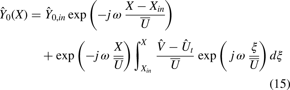
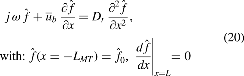
Analytical models for

F_{f}

and

F_{A}

are now derived. The fluctuation of fuel mixture fraction along the flame

\hat{f}

(which is not uniform due to the spread of residence time) is obtained from the linearization of the conservation equation for the fuel mixture fraction and the boundary condition at the fuel injection location

{\hat{f}}_{0}

\begin{aligned} j ω \hat{f} + {\bar{u}}_{b} \frac{\partial \hat{f}}{\partial x} = D_{t} \frac{\partial^{2} \hat{f}}{\partial x^{2}}, \\ with: \hat{f} (x = - L_{M T}) = {\hat{f}}_{0}, & {\frac{d \hat{f}}{d x} |}_{x = L} = 0 \end{aligned}

(20)

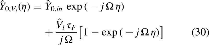
where it has been assumed that the field of fuel mixture fraction fluctuations is one-dimensional in direction

x

and that the mean velocity in the mixing section is uniform and equal to the velocity at the base of the flame. The solution of this equation, given for the fuel mixture fraction fluctuation

\hat{f} (x)

at a given location

x

normalised with the fuel mixture fraction fluctuation at the injection location

f_{0}

, i.e.

Z = \hat{f} / {\hat{f}}_{0}

, is:

Z = A_{1} \exp [α_{1} (x + L_{M T})] + A_{2} \exp [α_{2} (x + L_{M T})]

(21)

with:

α_{1, 2} = \frac{{\bar{u}}_{b}}{2 D_{t}} (1 \pm \sqrt{1 + 4 j \frac{D_{t} ω}{{\bar{u}}_{b}^{2}}})

(22)

The coefficients

A_{1}, A_{2}

are determined from the boundary conditions at the injection (

Z_{0} = 1

) and at a downstream location

L

sufficiently far from the flame where the fuel mixture fraction has decayed to very small value and where zero axial gradient (

d Z / d x |_{x = L} = 0

) can be imposed without affecting the distribution at the flame:

A_{1} = \frac{1}{1 - α_{1} / α_{2} \exp [(α_{1} - α_{2}) L]}

(23)

A_{2} = \frac{1}{1 - α_{2} / α_{1} \exp [(α_{2} - α_{1}) L]}

(24)

In the limit of

ω \to 0

we have:

α_{1} \to \frac{U}{D_{t}}, α_{2} \to 0; A_{1} \to 0, A_{2} \to 1

(25)

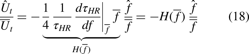
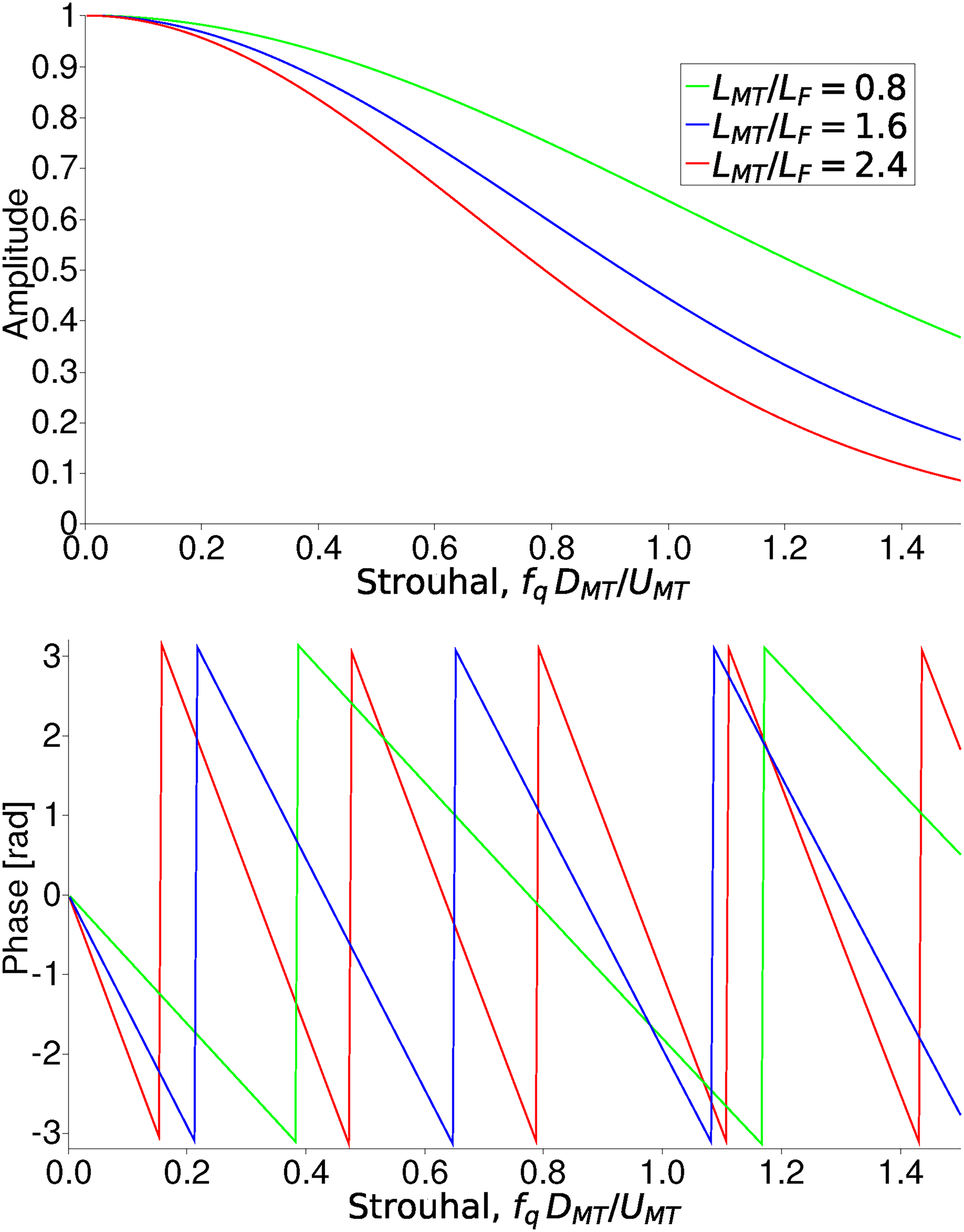
which yields

lim_{ω \to 0} Z = 1

We emphasize that, contrarily to models where the fuel mixture fraction is assumed to follow the Gaussian dispersion law, the fuel mixture fraction fluctuations is obtained here in a fully analytical fashion with the reduction in amplitude directly related to the turbulent diffusion coefficient $D_{t}$ . Figure 3 shows the distribution of $Z$ at the central point $P_{C}$ of a V-flame ( see Figure 1, bottom-right) for the same burner velocity ${\bar{u}}_{b}$ and diffusion coefficient $D_{t}$ but different values of the mixing section length $L_{M T}$ made non-dimensional with the flame length $L_{F}$ . Here, the phase shows a distribution perfectly in line with the time delay from fuel injection and the amplitude monotonically decreases with increasing frequency and distance due to the effect of turbulent diffusion.

Figure 3.

Frequency response of fuel mixture fraction ( $Z = \hat{f} / {\hat{f}}_{0}$ ) determined with relation (21) at the central point of a $V$ -shaped flame for increasing mixing section to flame length ratio.

The arguments $α (x + L_{M T})$ in (21) can be further elaborated in terms of non-dimensional parameters as:

\begin{aligned} α (x + L_{M T}) = R [η + S], x = η τ_{F} \bar{U} \cos β, \\ R = α τ_{F} \bar{U} \cos β, S = \frac{L_{M T}}{\bar{U} τ_{F} \cos β} \end{aligned}

(26)

where

S

is the ratio between residence time in the mixing section and the residence time along the flame.

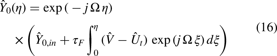
Replacing into expression (21) for $Z$ , with $R_{1}$ and $R_{2}$ from relation (26) using the values of $α$ given by relation (22), and then integrating along the flame gives:

F_{f} {\bar{A}}_{F} = A_{1} \exp (R_{1} S) G (R_{1}) + A_{2} \exp (R_{2} S) G (R_{2})

(27)

with

G (R)

G (R) = \int_{{\bar{A}}_{F}} \exp [R η] d A = \frac{r_{M} - r_{m}}{\sin β} r_{M} P (R; ψ)

(28)

where

ψ = r_{m} / r_{M}

and:

\begin{aligned} P (R; ψ) & = {(1 - ψ) \frac{1}{R^{2}} [\exp (R) (R - 1) + 1] \\ + ψ \frac{1}{R^{2}} [R \exp (R) - R]} \end{aligned}

(29)

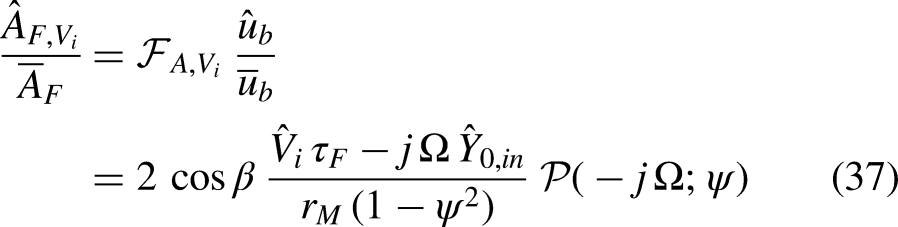
The contribution

F_{A}

to the FTF due to flame surface area fluctuations is obtained from relation (12) with

{\hat{Y}}_{0}

given by relation (16). This contribution can be split into a first part due to velocity fluctuations

\hat{V}

and a second one due to the turbulent flame speed fluctuations

{\hat{U}}_{t}

which can be expressed in terms of fuel mixture fraction fluctuations on the basis of relation (18). Regarding the first part, the velocity fluctuation orthogonal to the flame

\hat{V}

was decomposed in¹³ into an irrotational

{\hat{V}}_{i}

and a rotational

{\hat{V}}_{r}

contributions using the Helmholtz-Hodge decomposition.¹⁴ The irrotational velocity part

{\hat{V}}_{i}

is due to the pure acoustic perturbation which is characterized by wavelength much longer than the flame length, i.e. it can be considered uniform along the flame. The flame displacement

{\hat{Y}}_{0, V_{i}}

due to the irrotational velocity component is therefore given by:

{\hat{Y}}_{0, V_{i}} (η) = {\hat{Y}}_{0, i n} \exp (- j Ω η) + \frac{{\hat{V}}_{i} τ_{F}}{j Ω} [1 - \exp (- j Ω η)]

(30)

The second contribution is given by the turbulent flame speed part which, considering in base of relation (18) that

{\hat{U}}_{t} = - H {\bar{U}}_{t} Z {\hat{f}}_{0} / \bar{f}

, gives:

\frac{{\hat{Y}}_{0, U_{t}} (η)}{H \bar{U_{t}} τ_{F} ({\hat{f}}_{0} / \bar{f})} = \exp (- j Ω η) \int_{0}^{η} Z \exp (j Ω ξ) d ξ

(31)

and after replacing expression (21) for

Z

\begin{aligned} \frac{{\hat{Y}}_{0, U_{t}} (η)}{H {\bar{U}}_{t} τ_{F} ({\hat{f}}_{0} / \bar{f})} = A_{1} \exp (R_{1} S) L_{1} + A_{2} \exp (R_{2} S) L_{2} \end{aligned}

(32)

where

L = L_{1, 2}

is given by:

\begin{aligned} L & = \exp (- j Ω η) \int_{0}^{η} \exp [(R + j Ω) ξ] d ξ \\ = \frac{\exp (- j Ω η)}{R + j Ω} {\exp [(R + j Ω) η] - 1} \\ = \frac{1}{R + j Ω} {\exp (R η) - \exp (- j Ω η)} \end{aligned}

(33)

The derivative with respect to the independent variable

η

{\hat{Y}}_{0, V_{i}}

and

L

gives:

\frac{d {\hat{Y}}_{0, V_{i}}}{d η} = ({\hat{V}}_{i} τ_{F} - j Ω {\hat{Y}}_{0, i n}) \exp (- j Ω η)

(34)

\frac{d L}{d η} = \frac{R \exp (R η) + j Ω \exp (- j Ω η)}{R + j Ω}

(35)

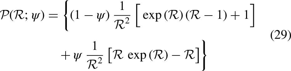
The contributions to the flame surface area due to irrotational velocity and to turbulent flame speed fluctuations can now be determined using relation (12) and the two previous relations (34) and (35). In case of velocity fluctuations

V_{i}

\begin{aligned} {\hat{A}}_{F, V_{i}} & = | \cot β | \int_{0}^{1} [(r_{M} - r_{m}) η + r_{m}] \frac{d {\hat{Y}}_{0, V_{i}}}{d η} d η \\ = | \cot β | ({\hat{V}}_{i} τ_{F} - j Ω {\hat{Y}}_{0, i n}) r_{M} P (- j Ω; ψ) \end{aligned}

(36)

where

P (- j Ω; ψ)

is given by relation (29) with

- j Ω

in place of

R

. Dividing by the mean flame surface area

{\bar{A}}_{F} = r_{M}^{2} (1 - ψ^{2}) / 2

, the velocity contribution to the flame surface area part of the FTF,

F_{A, V_{i}}

, is:

\frac{{\hat{A}}_{F, V_{i}}}{{\bar{A}}_{F}} = F_{A, V_{i}} \frac{{\hat{u}}_{b}}{{\bar{u}}_{b}} = 2 \cos β \frac{{\hat{V}}_{i} τ_{F} - j Ω {\hat{Y}}_{0, i n}}{r_{M} (1 - ψ^{2})} P (- j Ω; ψ)

(37)

It can be shown that the limit of this relation for

Ω \to 0

is equal to

{\hat{V}}_{i} / \bar{V}

. Given that for mass conservation

{\hat{V}}_{i} / \bar{V} = {\hat{u}}_{b} / {\bar{u}}_{b}

then it follows that

lim_{Ω \to 0} F_{A, V_{i}} = 1

The integration of relation (35) gives instead the two contributions below, each to be considered for the two values of $R = R_{1, 2}$ :

\frac{| \cot β |}{{\bar{A}}_{F}} \int_{{\bar{A}}_{F}} \frac{d L^{(B)}}{d r} r d r = 2 \frac{R}{R + j Ω} \frac{\cos β P (R, ψ)}{r_{M} (1 - ψ^{2})}

(38)

\frac{| \cot β |}{{\bar{A}}_{F}} \int_{{\bar{A}}_{F}} \frac{d L^{(A)}}{d r} r d r = 2 \frac{j Ω}{R + j Ω} \frac{\cos β P (- j Ω, ψ)}{r_{M} (1 - ψ^{2})}

(39)

In order to determine the contribution to the flame surface area due to turbulent flame speed fluctuations

{\hat{A}}_{F, U_{t}}

, relations (38) and (39) must be combined as indicated by (32) resulting in the sum of four terms. It can be finally shown that:

lim_{ω \to 0} \frac{{\hat{A}}_{F, U_{t}}}{{\bar{A}}_{F}} = H

(40)

then opposite to the direct contribution of

U_{t}

to the FTF (this equal to

- H F_{f}

with

lim_{ω \to 0} F_{f} = 1

In order to support the rest of the analysis, the contribution of turbulent flame speed fluctuations to the flame surface area part of the FTF is set as:

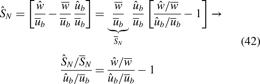
\frac{{\hat{A}}_{F, U_{t}} / {\bar{A}}_{F}}{{\hat{u}}_{b} / {\bar{u}}_{b}} = \frac{{\hat{A}}_{F, U_{t}} / {\bar{A}}_{F}}{{\hat{f}}_{0} / \bar{f}} \frac{{\hat{f}}_{0} / \bar{f}}{{\hat{u}}_{b} / {\bar{u}}_{b}} = F_{A, U_{t}} \frac{{\hat{f}}_{0} / \bar{f}}{{\hat{u}}_{b} / {\bar{u}}_{b}}

(41)

The final important contribution to the FTF is the one associated with the rotational component of the velocity fluctuation in the longitudinal plane. The physical mechanism behind this source of unsteady heat release is largely debated in the literature.¹² In this work we use a semi-empirical model based on the CFD results from¹³ where the velocity field in the longitudinal plane (under the assumption of axially symmetric flow) was decomposed into an irrotational and rotational parts via the Helmholtz-Hodge decomposition. The rotational part was shown to induce a Flame Surface Area frequency response behaving like the swirl number perturbation at the base of the flame. In this case, the swirl number perturbation acts on the vortex breakdown phenomenon, dynamically exciting the central recirculation region and therefore also the flame. In first approximation the swirl number perturbation

{\hat{S}}_{N}

at the base of the flame is given by

S_{N} ≃ w / u_{b}

) where

w

represents the radially averaged tangential velocity. The linearization of this expression yields:

\begin{aligned} {\hat{S}}_{N} = [\frac{\hat{w}}{{\bar{u}}_{b}} - \frac{\bar{w}}{{\bar{u}}_{b}} \frac{{\hat{u}}_{b}}{{\bar{u}}_{b}}] & = \underset{{\bar{S}}_{N}}{\underset{⏟}{\frac{\bar{w}}{{\bar{u}}_{b}}}} \frac{{\hat{u}}_{b}}{{\bar{u}}_{b}} [\frac{\hat{w} / \bar{w}}{{\hat{u}}_{b} / {\bar{u}}_{b}} - 1] \to \\ \frac{{\hat{S}}_{N} / {\bar{S}}_{N}}{{\hat{u}}_{b} / {\bar{u}}_{b}} & = \frac{\hat{w} / \bar{w}}{{\hat{u}}_{b} / {\bar{u}}_{b}} - 1 \end{aligned}

(42)

Assuming the mixing section compact with respect to the acoustic wavelength (for frequencies below

500 H z

, air temperature in the range of

700 K

, the acoustic wavelength is indeed larger than

≃ 1 m

), the axial velocity fluctuation

{\hat{u}}_{b}

, which propagates at the speed of sound, and its mean

{\bar{u}}_{b}

can be assumed uniform over the length of the mixing section and therefore equal to the respective upstream values at the swirler exit, i.e.

{\hat{u}}_{b} = {\hat{u}}_{b, 0}

and

{\bar{u}}_{b} = {\bar{u}}_{b, 0}

. At the swirler exit the ratio between tangential and axial velocity is fixed and imposed by the geometric swirl number of the swirling device, i.e.

w_{0} = S_{N, 0} u_{b, 0}

such that also

{\hat{w}}_{0} = S_{N, 0} {\hat{u}}_{b, 0}

and

{\bar{w}}_{0} = S_{N, 0} {\bar{u}}_{b, 0}

. Using finally these relations into the first term on rhs of relation (42) yields:

\frac{{\hat{S}}_{N} / {\bar{S}}_{N}}{{\hat{u}}_{b} / {\bar{u}}_{b}} = \underset{Z}{\underset{⏟}{\frac{\hat{w}}{{\hat{w}}_{0}}}} - 1

(43)

Given that the transport equation for tangential velocity is equal to the transport equation for fuel mixture fraction, the first term on rhs has the same behaviour of the non-dimensional fuel mixture fraction fluctuation

Z = \hat{f} / {\hat{f}}_{0}

. The second term (

- 1

) produces instead a non-monotonic modulation which gives zero swirl number fluctuation when

\hat{w}

at the base of the flame is in phase with

{\hat{u}}_{b}

and maximum when it is out of phase. Therefore, for analogy, the contribution to the FTF due to rotational velocity

{\hat{V}}_{r}

and associated with convection of tangential velocity fluctuations

F_{A, V_{r}}

has been modelled here as:

F_{A, V_{r}} = K F_{f} [\exp (- j ω τ_{M T}) - 1]

(44)

where

K

is a constant of order one.

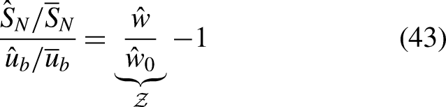
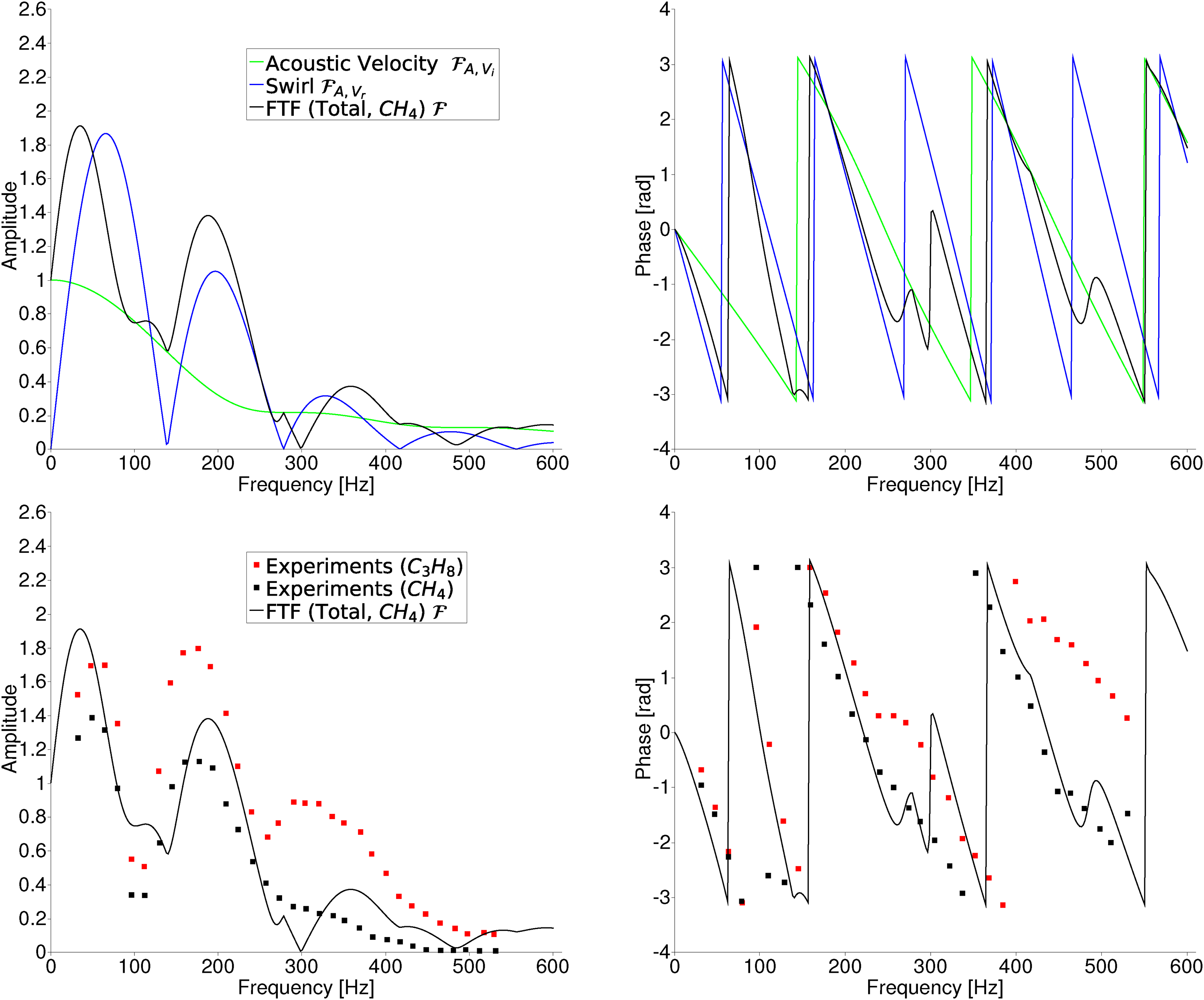
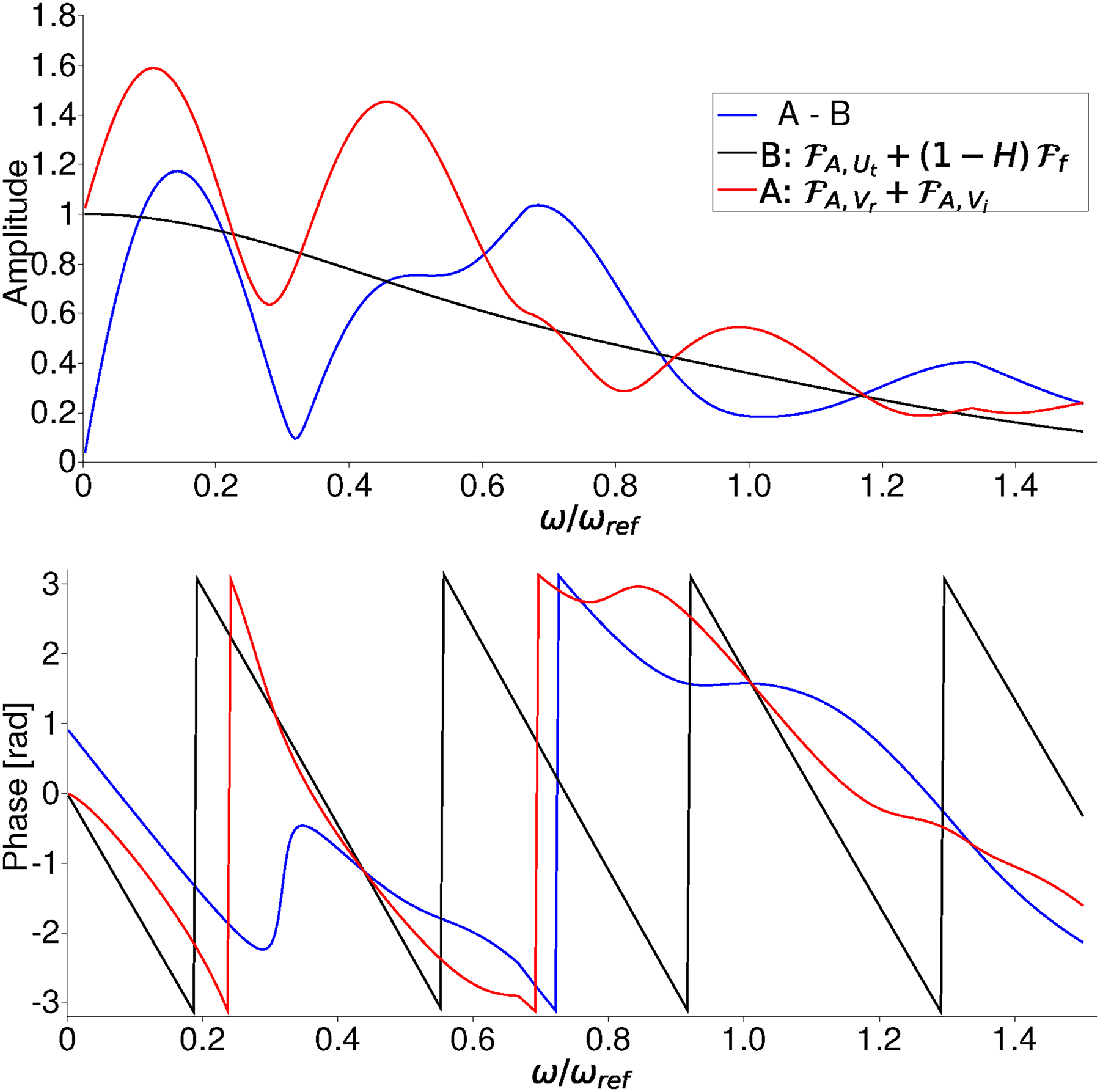
Summarizing, the semi-empirical relation (44) gives a contribution which is maximum when the tangential velocity fluctuation $\hat{w}$ transported by convection at the flame base is in phase with the axial velocity $\hat{u}$ (propagating at the much higher speed of sound) and zero when out of phase. Additionally, the maximum amplitude decreases with frequency in the same way of the transfer function of the fuel mixture fraction $F_{f}$ . A qualitative validation of this analytical model has been carried out against experimental data from¹⁵ in case of swirl stabilized perfectly premixed. The model is applied assuming uniform mean $\bar{V}$ and uniform irrotational velocity fluctuations ${\hat{V}}_{i}$ orthogonally to the flame while the flame angle is worked out from the flame images, see Figure 1 on the bottom right. The input parameters that completely determine the FTF under fully premixed conditions are given in the table in Figure 1. It must be pointed out that the residence time along the flame cannot be worked out from the available experimental information. Assuming that the velocity along the flame is same order of magnitude of the burner velocity, the flame residence time is proportional to the (known) residence time in the mixing section with proportionality constant given by the flame to mixing section length ratio. This constant has been worked out from the flame images in¹⁵ in the order of $L_{F} / L_{M T} ≃ 0.7$ leading to a value of $τ_{F} ≃ 5 m s$ against a residence time in the mixing section of $τ_{M T} = 7 m s$ . Figure 4 shows the two velocity contributions to the FTF and the total FTF obtained from their sum. The figure on the top shows that the contribution to the FTF due to the irrotational part of velocity is characterized by amplitude that monotonically decreases with increasing frequency. On the other hand, the contribution associated with the swirl number perturbation is dominant and characterized by amplitude having maxima and minima in line with the swirl number perturbation at the base of the flame. Additionally, the slope of the swirl number contribution indicates a larger time delay due to the fact that the origin of this perturbation is at the swirler exit while the contribution due to irrotational velocity works over the shorter time delay along the flame. The comparison with experiments is shown on the bottom part of the figure. The difference in the experiments between the case with $C H_{4}$ and the case with $C_{3} H_{8}$ as fuel is not very large. In case of fully premixed conditions in fact the linearized equation do not contain directly the effect of turbulent flame speed fluctuations, hence the difference in fuel composition does not play a large role. The analytical FTF, which is in fair agreement with the experiments, shows the importance of including the effect of swirl number perturbations in order to capture the experimental trend.

Figure 4.

FTF under fully premixed conditions. Top: contributions due to irrotational and rotational velocity components obtained with the present analytical model. Bottom: qualitative validation against experimental data from.¹⁵

Effect of fuel mass flow rate fluctuations

The flame transfer function is given by the fluctuating total heat release rate referenced to the axial velocity fluctuation at the flame base. The air flow impedance at the fuel injection location is given by the acoustic pressure to acoustic velocity ratio and can clearly have an effect on the relative importance of different contributions to the FTF. In fact, the higher this impedance is in amplitude in proximity of the fuel gas holes exit, the more important is the contribution of fuel mixture fraction fluctuations to the FTF in comparison to the effect of velocity fluctuations. Additionally, such impedance depends from the upstream geometry, for example from the length of the burner plenum. Given that for several reasons, the plenum geometry used in FTF measurements is usually not the same as the plenum of the real gas turbine, FTF transferability issues can arise from the test development environment to the real application conditions. It is shown below how the air side impedance at the location of fuel injection, which depends from the upstream geometry of the plenum, can influence the FTF via fluctuations in fuel mass flow rate. This exercise represents an initial attempt to justify FTFs distribution observed in previous experience which cannot be otherwise explained. A more complete exercise will be the subject of future work based on CFD analysis.

A typical test rig for measuring FTFs¹⁶ is characterized by a plenum having a cylindrical shape where acoustic wave propagation can be assumed one-dimensional and whose length is approximately $L_{P L} / D_{M T} = 4 - 6$ times the mixing tube diameter. As an application of the present analytical model, two different lengths of the plenum are considered here: $L_{P L} / D_{M T} = 4$ and $L_{P L} / D_{M T} = 5.3$ . Additional factors that can affect the impedance at the gas fuel injection which are not considered here are the inflow of air into the plenum and the presence of elements like a perforated screen which is typically positioned upstream the burner to make the approach flow more uniform.

At the fuel injection, the global fuel mixture fraction fluctuation ${\hat{f}}_{0}$ is given by the linearization of the ratio between the fuel mass flow rate divided the total flow mass flow rate:

f_{0} = \frac{{\dot{m}}_{F}}{{\dot{m}}_{F} + {\dot{m}}_{A}} \to \frac{{\hat{f}}_{0} / \bar{f}}{{\hat{u}}_{b} / {\bar{u}}_{b}} = (1 - \bar{f}) (\frac{{\hat{\dot{m}}}_{F} / \bar{{\dot{m}}_{F}}}{{\hat{\dot{m}}}_{A} / \bar{{\dot{m}}_{A}}} - 1)

(45)

where it is assumed that air mass flow rate fluctuations at fuel gas injection and base of the flame are equal, i.e. the mixing tube is compact with respect the acoustic wavelength. In order to include the effect of fuel mass flow rate fluctuations on the FTF, we refer to relation (17):

F = [F_{f} + F_{U_{t}} + F_{A, U_{t}}] \frac{{\hat{f}}_{0} / \bar{f}}{{\hat{u}}_{b} / {\bar{u}}_{b}} + F_{A, V_{i}} + F_{A, V_{r}}

(46)

and use (45) to include the effect of fuel mixture fraction fluctuations taking place at the location of fuel injection. Relation (45) shows two contributions: the first due to fuel mass flow rate fluctuations at the gas holes and the second due (

≃ - 1

) to air mass flow rate fluctuations. Fuel mass flow rate fluctuations on the FTF can be significant, even when they are classified as weak, i.e. even if fuel injection is ”stiff” due to high fuel pressure drop. If in fact the air impedance at the fuel injection location is high (

\hat{p} / \hat{u}

is high), the relative fuel mass flow rate fluctuation (relative to the mean) can still be quite high compared to the relative air mass flow rate fluctuation and then give a contribution to the FTF which is larger than the one given by velocity perturbations. The relation between these two contributions depends on the upstream boundary condition in the plenum such that the FTF, based on the definition (17), will not be uniquely defined as required for application in the thermo-acoustic stability analysis of the final gas turbine combustor.

The relation between fuel mass flow rate fluctuation and air slot impedance is determined below using a simplified model. The pressure drop at the gas holes is related to the fuel mass flow rate by the relation:

p_{u} - p_{3} = \frac{1}{2} \frac{{\dot{m}}_{F}^{2}}{ρ_{F} A_{f u e l}^{2}}

(47)

where

p_{u}, p_{3}

are respectively the pressure upstream and downstream the fuel gas holes and

A_{F}

the fuel gas holes effective area. It is assumed that pressure fluctuations in the fuel plenum upstream the gas holes are negligible (see for example¹⁷). Then the linearization of (47) yields:

{\hat{p}}_{3} = - \frac{{\hat{\dot{m}}}_{F} {\bar{\dot{m}}}_{F}}{ρ_{F} A_{F}^{2}}

(48)

which can be further elaborated as:

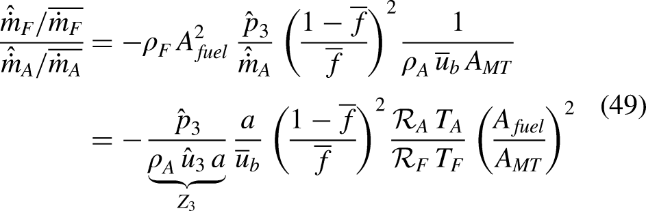
\begin{aligned} \frac{{\hat{\dot{m}}}_{F} / \bar{{\dot{m}}_{F}}}{{\hat{\dot{m}}}_{A} / \bar{{\dot{m}}_{A}}} & = - ρ_{F} A_{f u e l}^{2} \frac{{\hat{p}}_{3}}{{\hat{\dot{m}}}_{A}} {(\frac{1 - \bar{f}}{\bar{f}})}^{2} \frac{1}{ρ_{A} {\bar{u}}_{b} A_{M T}} \\ = - \underset{Z_{3}}{\underset{⏟}{\frac{{\hat{p}}_{3}}{ρ_{A} {\hat{u}}_{3} a}}} \frac{a}{{\bar{u}}_{b}} {(\frac{1 - \bar{f}}{\bar{f}})}^{2} \frac{R_{A} T_{A}}{R_{F} T_{F}} {(\frac{A_{f u e l}}{A_{M T}})}^{2} \end{aligned}

(49)

which shows that the fuel flow rate fluctuation relative to the air flow rate fluctuation at the gas holes is proportional to the opposite of the air slots impedance via a proportionality constant which depends linearly from the square of air to fuel mixture fraction ratio and from the square of the fuel to air area ratio (substantially both representing the effect of fuel velocity). The impedance

Z_{3}

at the gas holes is determined here considering a test rig with the following parameters:

L_{P L} / D_{M T} = 4.0 - 5.3

D_{P L} / D_{M T} = 3

L_{M T} / D_{M T} = 1.5

T_{a i r} / T_{f u e l} = 700 K / 300 K = 2.33

{\bar{u}}_{b} / a = 0.115

, fuel discharge coefficient

C_{D} = 0.79

and fuel gas holes to mixing tube geometric area ratio of

A_{F, g e o m} / A_{M T} = 1.5 E - 02

, which gives a fuel to air velocity ratio of the order of

u_{F} / {\bar{u}}_{b} = 2.3

for equivalence ratio

ϕ = 0.6

in line with values for industrial swirl burners. The impedance at the gas holes is worked out using first one-dimensional relations for wave propagation in the plenum:

\frac{{\hat{p}}_{2}}{ρ_{A} a} = \frac{1}{2} (\frac{{\hat{p}}_{1}}{ρ_{A} a} + {\hat{u}}_{1}) e^{- i K L} + \frac{1}{2} (\frac{{\hat{p}}_{1}}{ρ_{A} a} - {\hat{u}}_{1}) e^{i K L}

(50)

{\hat{u}}_{2} = \frac{1}{2} (\frac{{\hat{p}}_{1}}{ρ_{A} a} + {\hat{u}}_{1}) e^{- i K L} - \frac{1}{2} (\frac{{\hat{p}}_{1}}{ρ_{A} a} - {\hat{u}}_{1}) e^{i K L}

(51)

Z_{2} = \frac{e^{- i K L} - e^{i K L} + Z_{1} [e^{- i K L} + e^{i K L}]}{e^{- i K L} + e^{i K L} + Z_{1} [e^{- i K L} - e^{i K L}]}

(52)

where

K = 2 π f_{q} / a

, showing how the impedance at the inlet of the burner depends from the upstream plenum impedance and the plenum length

L_{P L}

. From section

S_{2}

the flow goes through a contraction until reaching the location of fuel gas injection in the burner at section

S_{3}

. Assuming this contraction as a compact element without losses, the impedance

Z_{3}

at the gas holes can be worked out from the following relations:

{\hat{u}}_{b} = {\hat{u}}_{2} / σ, {\hat{p}}_{3} + \bar{ρ} {\bar{u}}_{b} {\hat{u}}_{b} = {\hat{p}}_{2} + \bar{ρ} {\bar{u}}_{2} {\hat{u}}_{2} \to

(53)

Z_{3} = Z_{2} σ + \frac{{\bar{u}}_{b}}{\bar{c}} (σ^{2} - 1)

(54)

where

σ = A_{M T} / A_{P L}

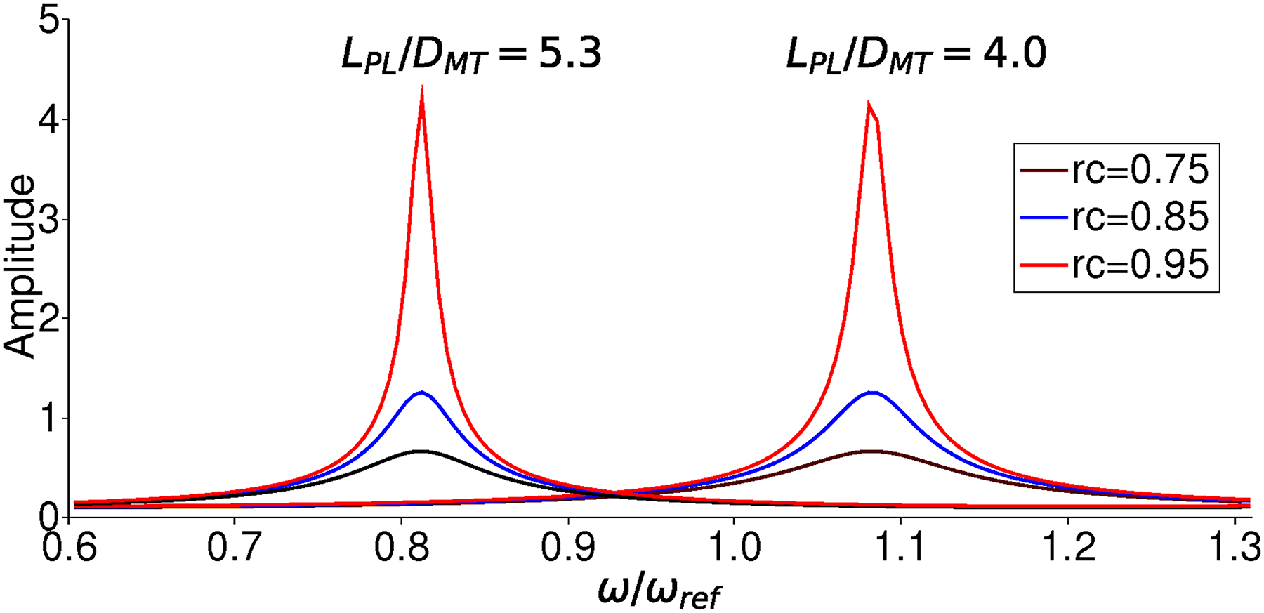
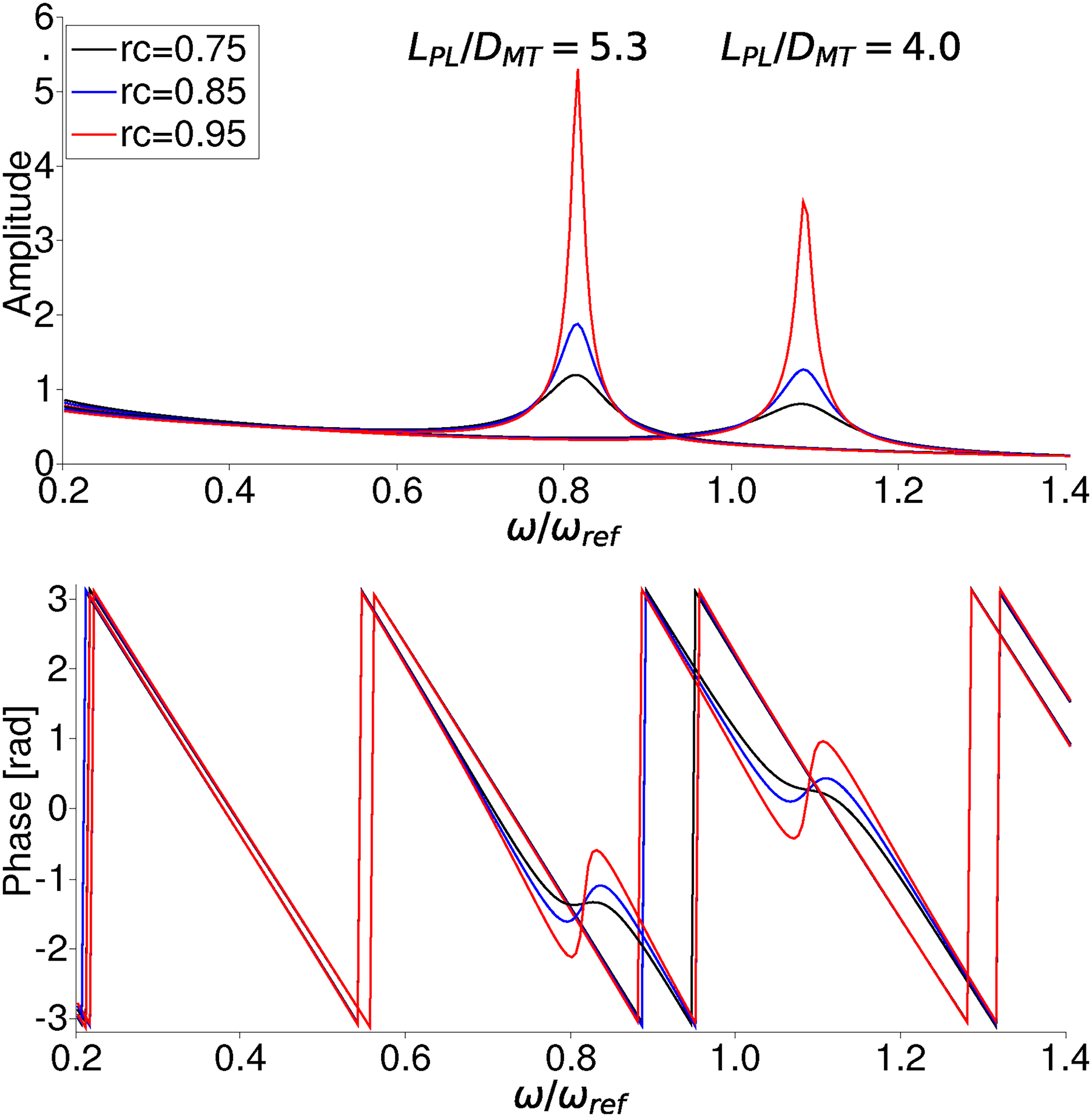
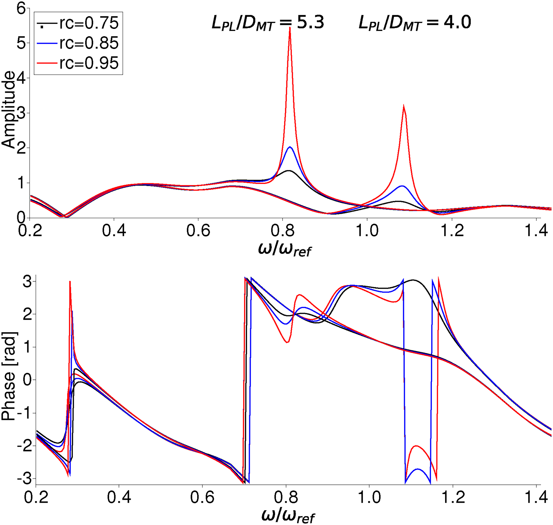
is the mixing tube to plenum area ratio. The plenum is a closed cavity with air injected from a pipe hence fully non-reflective acoustic conditions are difficult to achieve. In this analysis we consider values of the reflection coefficient upstream in the plenum in the range

r c = (Z_{1} + 1) / (Z_{1} - 1) = 0.75 - 0.95

. The case of fully reflective conditions (

r c = 1

) yields a pressure anti-node at the end of the plenum for

k L_{P L} = π

, i.e. for a non-dimensional frequency

f_{q} / f_{q, r e f} = a D_{M T} / (2 L_{P L} {\bar{u}}_{b})

(with

f_{q, r e f} = {\bar{u}}_{b} / D_{M T}

) which is equal to

0.8

in case of

L_{P L} / D_{M T} = 5.3

and to

1.08

in case of

L_{P L} / D_{M T} = 5.3

. Figure 5 shows the impedances at the section

S_{3}

positioned at the fuel gas holes for three different values of the reflection coefficient and the two different lengths of the plenum. The impedance distributions shows a sharp peak at the frequencies provided by the previous estimations. The frequency response of the fuel mixture fraction fluctuation at the section

S_{3}

is instead shown in Figure 6 for two lean values of the equivalence ratio. At the frequencies where the fuel injection location is a pressure anti-node, the transfer function of the fuel mixture fraction show a sharp increase in line with the impedance distribution. The peak values increase with decreasing equivalence ratio and increasing reflection coefficient at the section

S_{1}

. Away from these frequencies the fuel mixture fraction fluctuation is instead given just by air fluctuations, hence with amplitude equal to

1 - \bar{f}

and in phase opposition to the air mass flow rate fluctuation. The FTF is determined considering that reactants are consumed only by the inner flame anchored at the centreline (hence

ψ = r_{m} / r_{M} = 0

). The mixing tube length to diameter ratio is considered equal to

L_{M T} / D_{M T} = 1.5

, the flame angle is assumed as

β = 35^{o}

and the ratio between residence time along the flame and residence time in the mixing tube equal to

τ_{F L} / (L_{M T} / U_{M T}) ≃ L_{F} / L_{M T} ≃ 0.7

, which are typical values of an industrial burner (see for example¹⁸).

Figure 5.

Impedance $Z_{3}$ at fuel gas holes position $S_{3}$ .

Figure 6.

Frequency response of $({\hat{f}}_{0} / \bar{f}) / ({\hat{u}}_{b} / {\bar{u}}_{b})$ for two different lengths of the burner plenum, two different values of the equivalence ratio and upstream plenum reflection coefficient in the range $r c = 0.75 - 0.95$ .

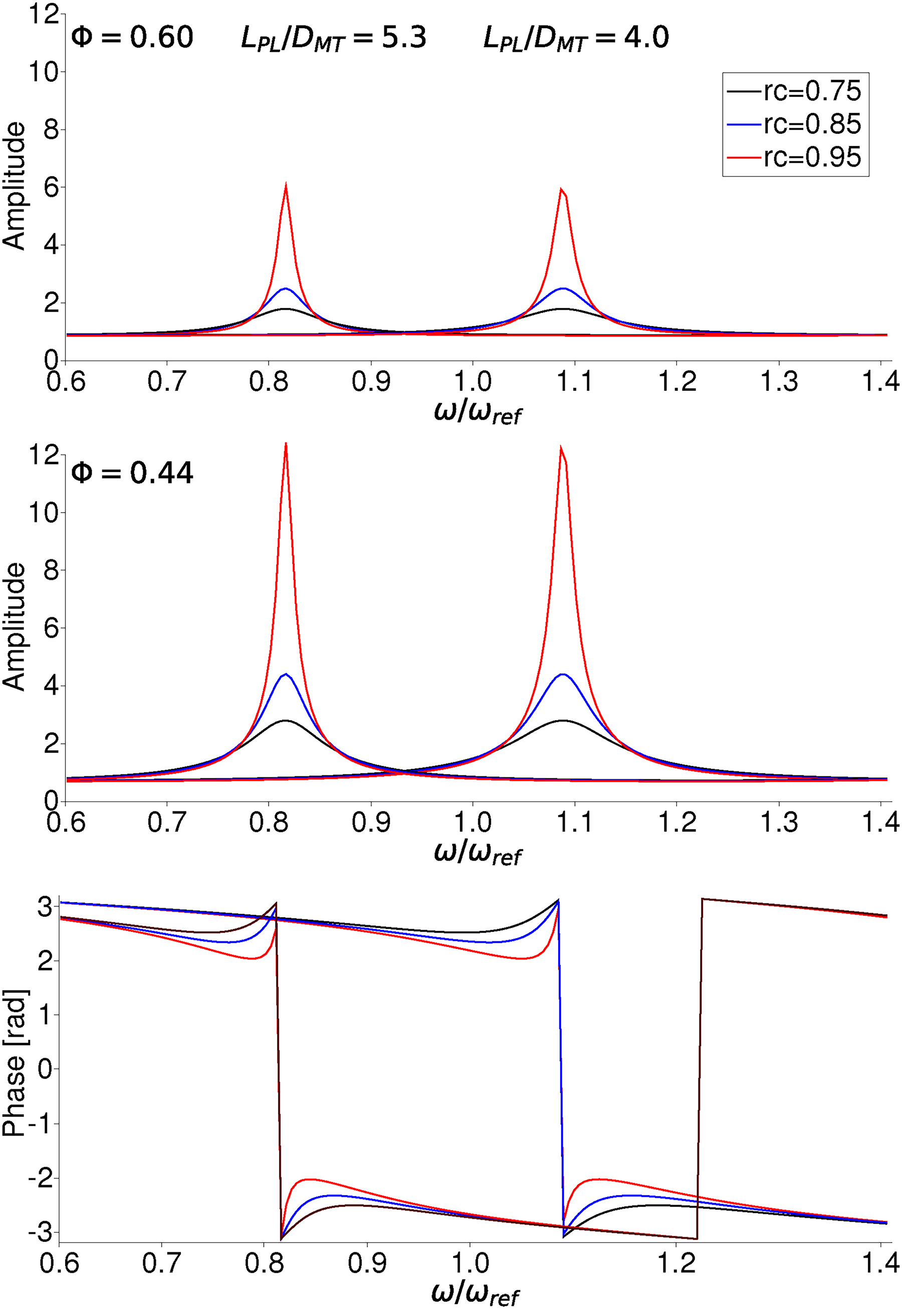
Figure 7 shows the fuel mixture fraction driven parts of the FTF (referenced to the fuel mixture fraction fluctuation ${\hat{f}}_{0} / \bar{f}$ at the fuel injection) for equivalence ratio $ϕ = 0.44$ . In the low to medium frequency range, the contribution directly due to the turbulent flame speed fluctuation is almost identical in amplitude and in phase opposition to the turbulent flame speed contribution to the flame surface area. In the high frequency range instead, the two contributions tend to be in phase and then add one to the other. For this reason, in the high frequency range, these two contributions ( $F_{A, U_{t}} - H F_{f}$ ) add to the direct contribution of fuel mixture fraction $F_{f}$ , increasing the overall amplitude. Figure 8 shows the total velocity contribution to the FTF (due to rotational and irrotational velocity components $F_{A, V_{i}} + F_{A, V_{r}}$ ), the total contribution due to fuel mixture fraction fluctuations, $(1 - H) F + F_{A, U_{t}}$ , referenced to fluctuations in fuel mixture fraction at the fuel injection location ( ${\hat{f}}_{0} / \bar{f}$ ) and the combination of these two. The distribution is in line with the one already seen in Figure 4 for fully premixed flame but with a limit of zero for $ω \to 0$ as it is required in case of technically premixed flames. Accounting also for the effect of fuel mass flow rate fluctuations at the fuel injection location gives the result, $[(1 - H) F_{f} + F_{A, U_{t}}] ({\hat{f}}_{0} / \bar{f}) / ({\hat{u}}_{b} / {\bar{u}}_{b})$ , shown in Figure 9 in case of the lowest equivalence ratio $ϕ = 0.44$ . These distributions are practically the same as the black line in Figure 7 with exception around the two frequencies where the response of ${\hat{f}}_{0}$ reaches a peak (see Figure 6).

Figure 7.

Contribution to the FTF for equivalence ratio $ϕ = 0.44$ due to direct effect of turbulent flame speed, direct effect of fuel mixture fraction and effect of turbulent flame speed on flame surface area.

Figure 8.

Contributions to FTF driven by fuel mixture fraction fluctuations (without effect of fuel mass flow rate fluctuations), velocity fluctuations and their combination.

Figure 9.

Contributions to FTF for equivalence ratio $ϕ = 0.44$ due to fuel mixture fraction fluctuations, including the effect of fuel mass flow rate fluctuations through the fuel gas holes.

Adding to these distributions also the contributions to the FTF due to rotational and irrotational velocity components gives finally the result shown in Figure 10. Also in this case, the total FTF shows high peaks in amplitude exactly at the frequencies where also the ratio $({\hat{f}}_{0} / \bar{f}) / ({\hat{u}}_{b} / {\bar{u}}_{b})$ has a peak due to the air flow impedance at the gas injection.

Figure 10.

Contributions to FTF for equivalence ratio $ϕ = 0.44$ due to fuel mixture fraction fluctuations (including also the effect of fuel mass flow rate fluctuations), velocity fluctuations and combined.

Without accounting for the effect of fuel mass flow rate fluctuations at the gas injection location, the fuel mixture fraction contribution to the total FTF is characterized by a rather smooth reduction in amplitude with frequency starting from the value of one at frequency zero. Also the contribution from irrotational velocity is decreasing in amplitude while the contribution due to swirl has a non-monotonic behaviour with peak values that however also decrease with frequency. A large increase in amplitude of the FTF is therefore possible at discrete values of the frequency due to the air flow impedance behaving in the same way.

Conclusions

The frequency response of technically premixed flames to acoustic excitation has been analysed. The investigation is carried out with an analytical model for the flame transfer function (FTF) obtained from the linearization of the mean reaction progress variable formation rate. The FTF is decomposed in several contributions, related to different physical mechanism driving the generation of unsteady heat release via acoustic excitation, see Figure 2. The two main governing mechanisms are due to velocity and fuel mixture fraction fluctuations along the mean flame. The effect of velocity is to generate unsteady heat release via flame surface area fluctuations. This part of the FTF can be further decomposed into two sub-parts driven respectively by the irrotational and rotational components of the velocity fluctuation orthogonal to the mean flame. Here, the effect of the rotational velocity component is accounted for with a semi-empirical model which links unsteady heat release to swirl number fluctuations at the flame base. Models have been also provided for the effect of fuel mixture fraction fluctuations that can generate heat release fluctuations in three different ways: directly via turbulent flame speed, directly via formation enthalpy fluctuations, indirectly via flame surface area driven by the turbulent flame speed. Fuel mixture fraction fluctuations at the flame are originated both by air and fuel mass flow rate fluctuations at the location of fuel injection. Given the definition of FTF (i.e. referenced to acoustic velocity at the flame base), the relative importance of the velocity and fuel mixture fraction driven part of the FTF can largely depend on the air flow impedance at the fuel injection location. Such impedance depends from the geometry upstream the burner. The fact that the plenum geometry used in FTF measurements is usually not the same as the plenum of the real gas turbine becomes therefore a potential reason for lack of FTF transferability from the test development environment to the real application conditions. This problem will be further investigated in future work with the help of CFD.

Footnotes

Declaration of Conflicting Interests

The authors declared no potential conflicts of interest with respect to the research, authorship, and/or publication of this article.

Funding

The authors received no financial support for the research, authorship, and/or publication of this article.

ORCID iD

Fernando Biagioli

Appendix

References

Keller

Egli

Althaus

. Vortex Breakdown As a Fundamental Element of Vortex Dynamics. Fluid Dyn Res 1988; 3(1-4): 31–42.

Syred

Beér

. Combustion in Swirling Flows: A Review. Combust Flame 1974; 23(2): 143–201.

Schuerman

Bellucci

Paschereit

. Thermoacoustic modeling and control of multi burner combustion systems, ASME paper 2003-GT-38688, 2003.

Paschereit

Schuermans

Polifke

Mattson

. Measurement of Transfer Matrices and Source Terms of Premixed Flames. J Eng Gas Turb Power 2002; 124(2): 239–247.

Huber

Polifke

. Dynamics of Practical Premix Flames, Part II: Identification and Interpretation of CFD Data. Int J Spray Combust Dynam 2009; 1(2): 229–250.

Kerstein

Ashurst

Williams

. Field Equation for Interface Propagation in An Unsteady Homogeneous Flow Field. Phys Rev A 1988; 37: 2728.

Liewen

. Nonlinear Kinematic Response of Premixed Flames to Harmonic Velocity Disturbances. Int Symp Combust 2005; 30(2): 1725–1732.

Cho

Lieuwen

. Laminar Premixed Flame Response to Equivalence Ratio Oscillations. Combust Flame 2005; 140: 116–129.

Semlitsch

Orchini

Dowling

Juniper

. G-equation Modelling of Thermoacoustic Oscillations of Partially Premixed Flames. Int J Spray Comb Dynam 2017; 9: 260–276.

10.

Albayrak

Polifke

. An Analytical Model Based on the G-equation for the Response of Technically Premixed Flames to Perturbations of Equivalence Ratio. Int J Spray Comb Dynam 2018; 10: 103–110.

11.

Zimont

. Gas Premixed Combustion At High Turbulence. Turbulent Flame Closure Combustion Model. Exp Therm Fluid Sci 2000; 21: 179–186.

12.

Kim

Santavicca

. Generalization of Turbulent Swirl Flame Transfer Functions in Gas Turbine Combustors. Comb Sci Techn 2013; 185(7): 999–1015.

13.

Biagioli

Scarpato

Syed

. Dynamic Response of Swirl Stabilized Turbulent Premixed Flames Based on the Helmholtz-Hodge Velocity Decomposition. Flow, Turbul Combust 2016; 96: 1005–1022.

14.

Batchelor

. An Introduction to Fluid Dynamics. Cambridge Mathematical Library. Cambridge University Press, 2000.

15.

Di Sabatino

Guiberti

Boyette

Roberts

Moeck

Lacoste

. Effect of Pressure on the Transfer Functions of Premixed Methane and Propane Swirl Flame. Combust Flame 2018; 193: 272–282.

16.

Komarek

Polifke

. Impact of Swirl Fluctuations on the Flame Response of a Perfectly Premixed Swirl Burner. J Eng Gas Turbines Power 2010; 132(6): 061503/1-7.

17.

Huber

. Impact of fuel supply impedance and fuel staging on gas turbine combustion stability. PhD Thesis, Technical University Munich, Germany, 2009.

18.

Bade

Wagner

Hirsch

Sattelmayer

Schuermans

. Influence of Fuel-Air Mixing on Flame Dynamics of Premixed Swirl Burners. Proceedings of ASME Turbo Expo 2014: Turbine Technical Conference and Exposition, paper GT2014-25381, 2014.