Inferring heat release dynamics from particle image velocimetry fields using physics-informed neural networks

Abstract

This study investigates the inference of heat release fields from time-averaged and time-resolved particle image velocimetry data using physics-informed neural networks. The method assimilates density fields using a continuity equation, from which heat release fields are calculated a posteriori using an enthalpy equation. The methodology is applied to data of a laminar, premixed methane V-flame of 1.53 kW thermal power and an equivalence ratio of 0.73 that is forced acoustically in the unsteady cases. Validation for the steady case is provided by comparing the assimilated density fields to fields obtained from the particle image velocimetry seeding concentration and by comparing the inferred heat release distribution to Abel de-convoluted OH* chemiluminescence images. The identified unsteady heat release rate fields are validated against global heat release readings from an OH*-filtered photomultiplier tube. This validation data is also transferred into a flame transfer function. The results indicate that dynamics of laminar, premixed flames can be identified solely from velocity data and detailed insights can be gained without any measurement of the heat release rate.

Keywords

Data assimilation PINN laminar V-flame flame dynamics

Introduction

Reacting flows are of interest in a wide range of engineering applications, including the aerospace and energy sectors.^1,2 The physics of these flows are highly complex, including not only the challenges known from non-reacting flows, such as turbulence, flow instabilities, and acoustic effects, but also additional phenomena arising from the chemical reactions. A particularly critical phenomenon in technical applications is thermoacoustic instability – a coupling between the acoustics of the combustion chamber and the heat release dynamics.^3–5 A classic mechanism leading to thermoacoustic instability includes the following feedback loop: an acoustic wave triggers vortex shedding at a location upstream near the flame anchoring point; the vortex is convected into the flame, where it distorts the flame and causes fluctuations in global heat release, thereby generating new acoustic fluctuations that can again induce upstream vortex shedding.

In industrial combustors, thermoacoustic instabilities must be avoided, as they can lead to increased harmful emissions and pressure pulsations that can cause structural damage to the combustion chamber,² potentially resulting in engine failure. Although numerical simulations that resolve acoustics, hydrodynamics, and heat release dynamics are feasible with today’s computing capabilities,⁶ they remain too costly for extensive parameter studies. As a result, low-order network models are often employed.^7–9 These models rely on a separation between the acoustic wave propagation and the flame’s response to acoustic excitation. By coupling both components in a feedback loop, the stability of the full system can be assessed and optimized.^7,10–13 The propagation of acoustic waves within a combustion chamber can be modeled with satisfactory accuracy using acoustic transfer functions derived from the Helmholtz equation. In contrast, the flame’s response to acoustic forcing, described by the flame transfer function (FTF), involves the interaction of the flow field, acoustics, and heat release dynamics, making it considerably more complex. Therefore, the FTF is often determined experimentally.

Experimentally, FTFs can be determined using either the multi-microphone method (MMM),¹⁴ which quantifies the acoustic transfer across the flame, or through optical diagnostic techniques.¹⁵ In both approaches, acoustic excitation is typically introduced into the test rig via loudspeakers or sirens, and the response of the flame is measured. A key advantage of optical methods is that, in addition to providing global input-output information in form of the FTF, they can also offer spatially resolved data. For example, when combining velocity measurements obtained via particle image velocimetry (PIV) with heat release measurements, commonly derived from chemiluminescence of the OH* radical for perfectly premixed methane flames, it becomes possible to investigate not only the FTF but also the local interaction between hydrodynamic structures and heat release fluctuations. However, such insightful measurements are complex and require the simultaneous use of a PIV system and OH* diagnostics. In this study, we investigate how information about heat release can be assimilated from velocity fields only, using physical laws and physics-informed neural networks (PINNs).¹⁶

Raissi et al.¹⁶ developed a methodology to solve partial differential equations (PDEs) within the training process of neural networks, known as PINNs. The core idea behind the method is to approximate physical quantities, such as a velocity field $u (x, r, t)$ using a neural network that takes spatial ( $x, r$ ) and temporal ( $t$ ) coordinates as input and returns the corresponding physical values ( $u$ ) as output. To ensure a physically meaningful approximation, governing PDEs are incorporated into the training process. This is done by evaluating the residuals of the PDEs at selected spatial and temporal points using the network’s predicted quantities and including these residuals in the loss function. This ensures that the training of the PINN, that is, the minimization of the loss function, leads to the output quantities approximating a solution of the imposed PDEs. The spatial and temporal derivatives that are required to evaluate the PDEs can be computed efficiently through automatic differentiation, which allows for the calculation of derivatives of the output quantities with respect to the input coordinates.

In addition to PDE residuals, other terms, such as the difference between predicted quantities and available measurement data, can be included in the loss function. This enables the use of PINNs for data assimilation tasks.^16,17 By defining a composite loss function that penalizes both deviations from data and residuals of PDEs, PINNs allow for the identification of physical quantities that are not directly measured. This has been successfully applied to various flows.^17–20

In the following a few selected studies are highlighted that focused on experimental data. For instance, Wang et al.²¹ assimilate the pressure field from time-resolved tomographic PIV measurements of the wake behind a hemisphere. von Saldern et al.²² demonstrate that PINN-based data assimilation is also effective for experimental mean flow data. They reconstruct the time-averaged azimuthal velocity, pressure and eddy viscosity field of a turbulent swirling jet using measurements of the axial and radial velocity components along with limited data of the azimuthal component. Steinfurth and Weiss²³ apply PINNs to reconstruct the three-dimensional mean velocity field over a backward facing ramp based on sparse measurements. Hasanuzzaman et al.²⁴ use PINNs to enhance PIV data of a turbulent boundary layer. Villié et al.²⁵ employ the method for artifact correction in MRI-based velocity measurements of a stenotic flow.

Data assimilation using PINNs has also been applied to time-averaged reacting flows, for example to infer turbulent combustion closures from available measurements.^26,27 von Saldern et al.²⁸ employ a PINN to approximate the time-averaged flow field of a reacting hydrogen jet. The assimilation extends the limited PIV measurement domain, enabling a subsequent resolvent analysis of low-frequency structures. Yadav et al.²⁹ also apply PINNs to reconstruct the flow fields of laminar and turbulent flames from sparse data. In their study, a reaction rate lookup table is used for the laminar case, while an eddy break-up model is employed for the turbulent case. Tathawadekar et al.³⁰ apply PINNs to assimilate the time-resolved velocity field of an unsteady laminar flame based on numerical data for the density, pressure, and temperature fields.

Based on the current literature on PINN-based data assimilation in reacting flows, three key challenges can be identified. First, studies focusing on turbulent cases typically rely on time-averaged velocity fields, even though the governing equations are based on density-weighted Favre averages. Second, most studies either consider steady flows or use numerical data for unsteady cases in which all relevant physical quantities are available and can be included in the training process. Third, the assimilation frameworks often involve multiple governing equations, including continuity, momentum, and energy equations, resulting in high computational cost during training.

In the present study, we aim to extract heat release dynamics from PIV measurements using a computationally efficient data assimilation framework. To avoid complications associated with the first challenge, we focus on a laminar flame, where time-resolved data can be used directly without the need for Favre averaging. We address the second and third challenges by extending PINN-based assimilation to unsteady, experimental reacting flows while reducing the complexity and cost of the training process. From a practical perspective, this objective is highly relevant, as the interaction between the flow field and heat release is central to understanding flame dynamics and determining the FTF. In addition to estimating the heat release rate, the proposed framework also provides access to the density and temperature fields.

The remainder of this article is structured as follows. First, the experimental database is described. In the Assimilation Methodology section, the governing equations and the details of the network training procedure are presented. The Results section begins with PINN-based assimilation of the heat release rate using stationary PIV data. Additional results based on harmonically forced data are presented in the subsequent section. The results are discussed in detail, and the assimilation methodology is validated through a multi-step approach. Finally, conclusions are drawn in the last section.

Experimental data set: Laminar methane flame

The methodology is applied to data from a laminar, premixed methane V-flame of 1.53 kW thermal power and an equivalence ratio of 0.73. A sketch of the test rig and an image of the laminar V-flame stabilized at the combustor outlet are shown in Figure 1. Upstream of the nozzle, the setup includes a honeycomb structure followed by a converging nozzle, designed to suppress velocity fluctuations and maintain a laminar flow. The nozzle has an exit diameter of $25$ mm and features a center-body along the axis to stabilize and anchor the flame. The radius of this bluff body is $2$ mm. To excite the flame acoustically, a loudspeaker is attached to the bottom of the combustor’s mixing chamber. It is operated with a mono-frequent harmonic signal at six different frequencies (19, 31, 47, 67, 91, and 137 Hz). For each frequency, measurements are performed at different forcing amplitudes by varying the electrical power supplied to the speaker. In the present study, however, we focus on one forcing amplitude per frequency, selected such that a clear and well-defined flame response is observed in the data at small velocity fluctuations.

Figure 1.

Sketch of the laminar V-flame test rig, image of the laminar methane flame, and overview of the available measurement data for forced and steady configurations.

The reacting flow is characterized by means of different measurement techniques. The velocity field is acquired through PIV. The dataset contains 2000 snapshots of the velocity field for the steady case and 4368 snapshots for each forcing frequency. For the forced cases, the sampling rate is varied linearly with the forcing frequency from 200 to 1373 Hz to capture $\sim$ 400 periods for each case. The processed PIV velocity field is captured on an equidistant cartesian grid with 63 times 63 points. Assuming axissymmetry and excluding erroneous measurement points at the upstream boundary results in an axial–radial grid of 51 times 32 points with a spatial resolution of $Δ x = Δ r = 1.48$ mm.

To acquire density fields, no direct measurements are available. However, in the upstream region, an estimate is obtained for the steady case by time-averaging the PIV particle images. These capture the scattered light intensity of the seeding particles.^31–33 This method only provides a rough estimate of the actual density, as it infers fluid density from the reflected light distribution. The estimate could be improved by subtracting the light emitted by the flame and the laser to remove contributions not related to particle reflections. However, this would require additional measurements showing only the flame or only the laser light, which are not available for the present setup.

For the configuration without acoustic forcing, 500 snapshots of the spatially resolved heat release rate are obtained by acquiring chemiluminescence of the OH* radical through a band pass-filtered UV-camera. The OH* field is resolved on an axial–radial grid of size 702 times 383 pixels with a resolution of $0.07$ mm in between measurement points. The data without forcing are processed to acquire time-averaged fields of velocity (from PIV), density estimates (from time-averaged captures of the PIV seeding concentration) and heat release (from the Abel de-convoluted OH* chemiluminescence images). Although the flame is laminar and steady, time averaging is used to suppress measurement noise and small fluctuations caused by external disturbances that amplify in the shear layers.

For the forced configurations, no spatially resolved OH* data is available. Instead, time-resolved global OH* values are recorded at a sampling rate of $8192$ Hz with an OH*-filtered photomultiplier tube. The PIV data and the global OH* data from the acoustically excited configurations are phase-averaged by cross-correlation with the driving signal of the speaker. For this, the instantaneous signals are sorted into discrete phase bins and subsequently averaged. The number of bins reflects a trade-off between temporal resolution and statistical convergence. Here, values of $N_{t} = 12$ , 24, and 48 bins are considered, of which only selected cases are used for PINN training. By defining a reference position for velocity fluctuations, these data can also be processed to obtain an estimate of the flame transfer function. An overview of the measurement techniques applied to the forced and steady configurations is given in the table in Figure 1.

The proposed methodology infers spatially resolved, and both, time-averaged and time-resolved heat release fluctuations using the PIV velocity fields as inputs. For the steady case, the procedure is validated by comparison with the OH* images and the density estimates from the PIV snapshots. For the forced cases, the phase-averaged global OH* value is used for validation.

Assimilation methodology

This section outlines the methodology for assimilating heat release dynamics from PIV velocity measurements. First, the governing equations used in the assimilation framework are introduced. Then, details regarding the loss function and the training procedure of the PINNs are provided.

The code used throughout this study is based on our publicly available in-house PINN code (https://git.tu-berlin.de/pida-group/), originally published by Klopsch et al.³⁴ and adapted for the present work.

Governing equations

To extract the heat release from the velocity measurements, we focus on the continuity equation

\frac{\partial ρ}{\partial t} + \nabla \cdot (ρ u) = 0

(1)

in which

ρ

denotes the density and

u

denotes the velocity vector. Since velocity information is provided by the PIV data, the density can be inferred from equation (1) given appropriate boundary conditions. To keep the assimilation process as computationally efficient as possible, equation (1) is the only governing equation included in the loss function during training.

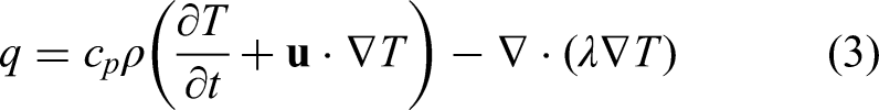
In a subsequent step, the trained PINN is used to compute the heat release. To this end, the temperature field $T$ is first calculated from the assimilated density by applying the ideal gas law,

T = \frac{p}{R ρ}

(2)

where

p

denotes pressure, and

R

the specific gas constant. Both pressure and the gas constant are assumed to be constant across reactants and products, which is a reasonable approximation for a laminar methane flame. In fact, a one-dimensional flame simulation using Cantera showed that the specific gas constant varies by <3% across the reaction zone for the considered composition (not shown).

The heat release rate $q$ is then computed from the enthalpy equation, which reads

q = c_{p} ρ (\frac{\partial T}{\partial t} + u \cdot \nabla T) - \nabla \cdot (λ \nabla T)

(3)

where

c_{p}

is the specific heat capacity at constant pressure and

λ

is the thermal conductivity. Since the neural network provides a continuous and differentiable approximation of the velocity and density fields, and thus, via equation (2), the temperature field, equation (3) can be directly evaluated to compute the heat release rate

q

. To evaluate equation (3), the heat capacity is assumed constant, which is reasonable for methane-air flames. The thermal conductivity

λ

, in contrast, changes more significantly across the flame. Its value depends on both gas composition and temperature. Since the spatial distribution of gas composition is not known,

λ

is only approximated from the inferred temperature field. For simplicity, a linear function of temperature is used, the coefficients of which are obtained by fitting data for the reactants and products as shown in Figure 2. The reactant composition corresponds to an equivalence ratio of

ϕ = 0.73

, while the product composition is derived from the chemical equilibrium of an adiabatic reaction. For methane-air combustion, the difference in thermal conductivity between products and reactants is relatively small, so that this approximation introduces only a minor inaccuracy.

Figure 2.

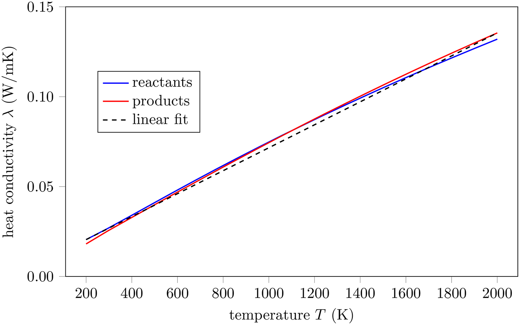
Temperature dependence of the heat conductivity of reactants and products for a methane-air flame with equivalence ratio $ϕ = 0.73$ . Black line shows the linear fit used for heat release calculations.

PINN setup—steady case

As a first step, the heat release field is assimilated using the steady data. This provides a baseline for evaluating the performance of the framework and analyzing its strengths and potential limitations.

To approximate the velocity vector and density field, a neural network is constructed that maps the spatial coordinates to the flow quantities,

[u_{x, α}, u_{r, α}, ρ_{α}] = N_{α} (x, r)

(4)

where

x

and

r

denote the axial and radial coordinates, respectively. The flow is assumed to be axisymmetric. The neural network is represented by

N_{α}

, where the subscript

α

indicates the dependence on the trainable parameters. These parameters are optimized during training by minimizing the total loss function,

α * = argmin \underset{L_{t o t a l}}{\underset{⏟}{β_{D} L_{D} + β_{P} L_{P} + L_{B C}}}

(5)

where

β_{D}

and

β_{P}

are weight factors for the data loss

L_{D}

and physics loss

L_{P}

, respectively. The term

L_{B C}

accounts for the boundary conditions. In the following, the individual terms contributing to the loss function are described in detail. Figure 3 shows the locations in the domain where the loss terms are evaluated, together with streamlines of the measured velocity field in the background.

Figure 3.

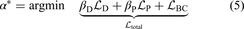
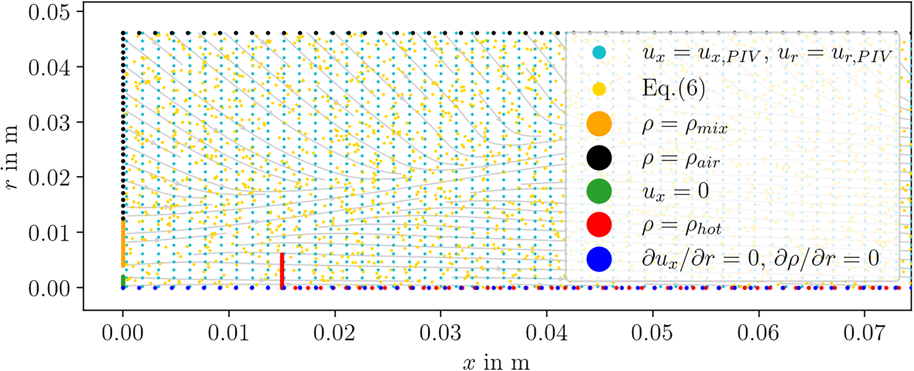
Location at which the individual loss terms in equation (5) are evaluated. The streamlines in the background show the measured velocity field.

The data loss term is based on the PIV measurements. It is computed as the mean squared difference between the predicted fields from the PINN and the corresponding measured velocity fields. For evaluating this term, all quantities are normalized. Each variable is scaled by its respective maximum value, such that the network outputs and inputs lie within the range of $0$ to $1$ . Since no direct measurements of the density field are available, the density is normalized using the reference value of air at 300 K, denoted as $ρ_{air}$ , which is assumed to represent the maximum value within the flow. This normalization makes network training easier, as the absolute values of the individual variables do not need to be learned. The 1632 PIV grid points used to evaluate the data loss are indicated by cyan markers in Figure 3.

To evaluate the physics loss, the PINN-approximated velocity and density fields are substituted in the steady continuity equation

\begin{aligned} e_{1} = & ρ_{α} (r \frac{\partial u_{r, α}}{\partial r} + r \frac{\partial u_{x, α}}{\partial x} + u_{r, α}) \\ + r u_{x, α} \frac{\partial ρ_{α}}{\partial x} + r u_{r, α} \frac{\partial ρ_{α}}{\partial r} \end{aligned}

(6)

where

e_{1}

denotes the residual. To avoid division by zero at the centerline, the continuity equation is multiplied with the radial coordinate. The mean squared residual forms the physics loss

L_{P}

. This term is evaluated in physical units. It should be noted that multiplying by the radial coordinate introduces a weighting of approximately

10^{- 3}

. The

2000

points at which the residual is computed are shown as yellow markers in Figure 3.

The velocity field, together with the continuity equation, defines the density field up to a constant offset along each streamline. To further constrain the density field, additional boundary conditions are imposed. These are incorporated into the boundary loss term $L_{B C}$ .

Ambient fluid entrained from the surroundings is assumed to have the density of air, $ρ_{a i r}$ . The corresponding 80 points at which this boundary condition is evaluated are shown as black markers in Figure 3. The orange markers denote locations near the nozzle inlet, where the density is set to that of the premixed methane-air mixture, $ρ_{m i x}$ which differs from $ρ_{a i r}$ by < $4 %$ . Since the flame anchors close to the bluff body near the nozzle exit, the mixture density is not imposed at the full upstream boundary. This is because heat conduction is expected to preheat the incoming fluid in the region close to the flame, resulting in a lower density. To still constrain the streamlines near the centerline, the density is specified downstream of the flame, where the gas is assumed to have reached the adiabatic flame temperature and to be composed of the equilibrium reaction products. These $70$ boundary points which correspond to the hot gas density, $ρ_{h o t}$ are shown as red markers in Figure 3.

Additional boundary conditions include zero axial velocity just downstream of the bluff body (10 green markers), and zero radial gradients of the axial velocity and density fields along the centerline (50 blue markers), as shown in Figure 3. All boundary loss terms are evaluated in physical units and are computed as the mean squared error between the specified and PINN-predicted values.

The objective of the PINN training is to infer the density field from the velocity data. To support this goal, an accurate approximation of the velocity field must first be achieved. This is ensured by prioritizing the data loss in the training process, setting the weight for the data loss to $β_{D} = 10$ , and the weight for the physics loss to $β_{P} = 0.1$ . These values were determined empirically through trial-and-error and are not universal, particularly because the data loss is evaluated in normalized units, whereas the physics loss is computed in physical units. They are chosen such that the weighted data loss dominates all other terms in the composite loss function over the entire training process.

A fully connected neural network is used, consisting of five hidden layers with 10 neurons each and tanh activation functions, resulting in a total of 503 trainable parameters. The comparatively small network size is chosen to limit the model complexity and thereby reduce the propagation of measurement artifacts in the velocity field into the inferred density field. This aspect is discussed in more detail in the Results section. The training procedure includes 464 iterations using the ADAM optimizer with mini-batching, followed by 30,000 full-batch steps using L-BFGS. The training process requires approximately half an hour when executed on a single core of a MacBook Air (2025, M4).

Figure 4 shows the evolution of the individual weighted loss terms during training. The loss values are recorded at every function call, which is why their count exceeds the number of training iterations. The vertical dotted line indicates the transition from ADAM to L-BFGS optimization.

Figure 4.

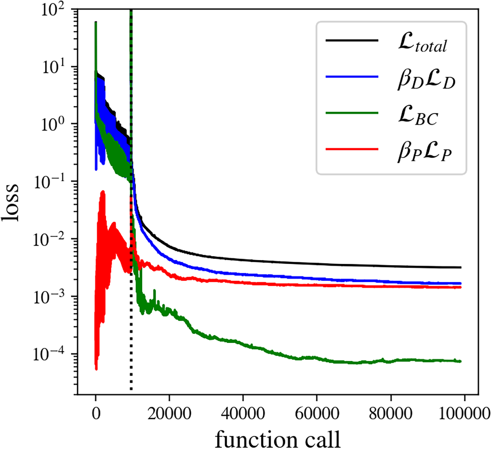
Losses of the composite loss function, equation (5) plotted over number of function calls. The dashed vertical line denotes the separation between ADAM and L-BFGS training phase.

As intended, the data loss dominates the total loss throughout the training. This prioritization is achieved through the chosen weighting factors $β_{D}$ and $β_{P}$ . It ensures that the network accurately fits the velocity data, thereby enabling inference of the density field from the measured values. During the ADAM phase, the physics loss initially increases, indicating that it is largely ignored by the optimizer. In the second phase, as the data loss becomes sufficiently small, the physics loss gains relative importance and is also minimized. After $\sim 8 \times 10^{4}$ function calls, the total loss flattens, indicating convergence of the training process.

PINN setup—unsteady cases

For the unsteady cases, a similar approach is employed. However, all physical quantities now depend on both space and time, which means the neural network features an additional input:

[u_{x, α}, u_{r, α}, ρ_{α}] = H_{α} (x, r, t)

(7)

Since the network now has one more input dimension, the architecture was extended from 10 to 40 neurons per layer. Temporal periodicity of the approximated velocity and density fields is enforced in the architecture via a coordinate embedding using a single sine and cosine function for the time input

(\sin (ω_{f} t), \cos (ω_{f} t))

, where the forcing frequency

ω_{f}

is prescribed for each case. Due to the subsequent nonlinear

\tanh

activation functions, the output remains periodic but is not restricted to a single-frequency oscillation and higher harmonics can appear. The idea behind embedding the periodicity in the network architecture and prescribing the oscillation frequency is to integrate this known characteristic directly into the model in order to improve the training process. Apart from these changes, the rest of the architecture remains as described in the previous section for the steady case. In total, the networks used for the unsteady cases have 6883 trainable parameters.

The network parameters are obtained, as described in equation (5), by minimizing a composite loss function, where the individual terms are extended due to the time dependence. The data loss now includes the phase-averaged PIV data, which provide velocity fields at each phase angle. As in the steady case, the data loss term is weighted by a factor of 10.

The physics loss is again defined as the mean squared residual of the continuity equation, which now also includes the time derivative term:

\begin{aligned} e_{2} = & ρ_{α} (r \frac{\partial u_{r, α}}{\partial r} + r \frac{\partial u_{x, α}}{\partial x} + u_{r, α}) \\ + r u_{x, α} \frac{\partial ρ_{α}}{\partial x} + r u_{r, α} \frac{\partial ρ_{α}}{\partial r} + r \frac{\partial ρ_{α}}{\partial t} \end{aligned}

(8)

The residual is evaluated over the space–time domain at 10,000 randomly sampled points. Of these, 3000 are distributed across the entire domain, while 7000 are concentrated in the upstream two-thirds of the spatial domain, where the flame is located. The physics loss weight $β_{P}$ is set to 1.

Boundary conditions are evaluated at the same spatial locations as in the steady cases. However, while they were previously sampled along spatial lines, they must now also be evaluated over time. To this end, the boundary conditions are randomly sampled on space–time planes and included in the loss function. These planes correspond to the spatial lines shown in Figure 3, extended into the time dimension. Specifically, the inlet density boundary condition $ρ = ρ_{m i x}$ is evaluated at 200 points and the air entrainment condition $ρ = ρ_{a i r}$ at 450 points. The hot gas density condition $ρ = ρ_{h o t}$ is enforced at 200 points along the axis and another 200 points within the domain. All remaining symmetry axis conditions are evaluated at 300 points. For the unsteady cases, the velocity boundary condition at the bluff body is omitted. This choice is motivated by the high sensitivity of the PINN training to this region (for the steady case), and by the fact that the measured velocity data in this area do not fully satisfy the prescribed condition.

The networks are trained for 50 epochs using the Adam optimizer, followed by 25,000 iterations of L-BFGS. Training takes a few hours on a single core of a MacBook Air (2025, M4). A separate network is trained for each excitation frequency.

Results

In this section, the main results of the study are presented and discussed. Following the structure of the Methodology section, we begin with the assimilation of the steady case, before proceeding to the unsteady cases.

Steady flow assimilation

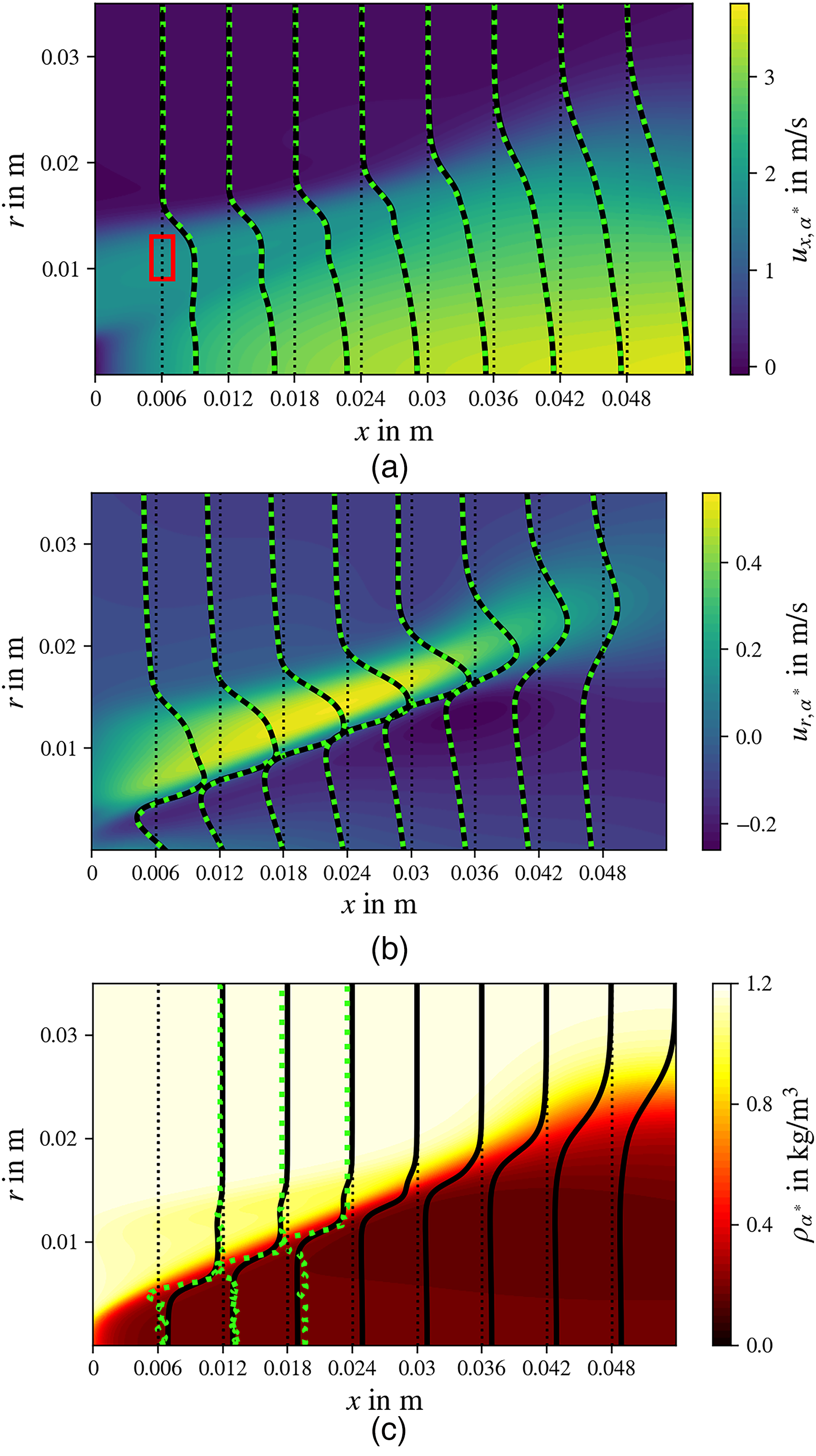
Figure 5 shows contour plots of the assimilated axial velocity $u_{x, α *}$ , radial velocity $u_{r, α *}$ , and the inferred density field $ρ_{α *}$ , where the asterisk indicates the use of the optimized network parameters through training (see equation (5)). The black vertical lines show normalized radial profiles that are compared to the corresponding measured profiles shown as green dotted lines.

Figure 5.

From top to bottom: PINN-predicted axial velocity, radial velocity, and density fields. Black vertical lines indicate the normalized profiles extracted from the PINN solution, while green dotted lines show the corresponding profiles from the PIV measurements. Black dotted lines indicate the location at which the profiles are compared. The red rectangle in the top plot denotes the control volume used to compute the characteristic velocity in eqation 10.

Figure 5 shows that the PINN approximates the PIV data very well for both velocity components across the entire domain. This accuracy is primarily attributed to the high weighting applied to the data loss term during training.

Regarding the density field, the PINN infers a physically meaningful distribution, characterized by a distinct V-shaped separation between regions of high and low density. This interface corresponds to the flame front, where the exothermic reactions cause a sharp temperature rise and, consequently, a drop in density. A comparison between the PINN-assimilated and seeding-based density profiles (green dotted lines) shows good agreement: the location of the density gradient is accurately captured by the PINN. However, the gradient in the seeding data appears more pronounced, and the profiles exhibit a slight undershoot not present in the PINN results. While the undershoot is likely not a physical effect but rather a byproduct of the qualitative nature of seeding-based density estimation, the smoothed gradient in the PINN results is likely due to the coarse resolution of the PIV data (see Figure 6). Since the density is inferred solely from the velocity field via the continuity equation, resolving a sharp transition across a laminar flame front becomes challenging when the velocity field lacks sufficient resolution in this region. Nevertheless, Figure 5 demonstrates that the PINN successfully assimilates the flow field, yielding a physically plausible density distribution.

Figure 6.

Heat release rate from the OH* chemiluminescence measurement (upper half) and from the PINN-inferred density field (lower half). Blue dots denote the PIV grid. PINN: physics-informed neural network; PIV: particle image velocimetry.

In the next step, the temperature field is computed from the density field using the ideal gas law, equation (2). Subsequently, the heat release rate is determined from the energy equation, equation (3), where the time derivative is neglected as the flow is assumed to be steady. In the final step, negative values are set to zero as they are considered unphysical. It is important to note that all required operations for evaluating these equations can be performed directly within the PINN framework using automatic differentiation, without the need for any discretization scheme.

Figure 6 compares the heat release rate derived from the PINN-approximated field (lower half) with the OH* chemiluminescence measurements (upper half). Overall, the PINN results show good qualitative agreement with the measured data. Key features such as the flame anchoring point and the flame angle are well captured. The qualitative position and characteristic V-shaped structure of the flame are reproduced. However, there are some notable differences between the fields. The assimilated flame appears thicker than the measured OH* signal, particularly near the anchoring region. The PINN-predicted flame is also slightly longer.

The increased flame thickness observed in the assimilated results can be explained by the limited resolution of the PIV measurements. While the OH* field is spatially well resolved, the number of PIV data points within the reaction zone, see blue grid points in Figure 6, is very limited. At most locations, only two PIV points lie within the reaction zone. Consequently, the velocity gradient across the flame front is estimated from sparse data. Additionally, PIV processing using interrogation windows inherently imposes a spatial low-pass filter on the velocity field. Furthermore, temporal averaging of the PIV data, applied to filter out small disturbances, has an additional smoothing effect on the velocity gradients. In the presented assimilation framework, the velocity data are effectively treated as ground truth (high weighting) from which the density field is inferred. As a result, these combined smoothing effects propagate into the assimilation process and lead to less pronounced gradients in the inferred density (see Figure 5) and consequently, in the temperature field. The smoothing effects are even more pronounced for second-order derivatives, which scale with the square of the wavenumber and are, therefore, more strongly damped by spatial low-pass filtering. Since the heat release rate is estimated from first- and second-order derivatives of the temperature field (see equation (3)), these effects propagate through the postprocessing and lead to a thickened, smeared-out flame front, explaining the differences to the highly resolved OH* images, shown in Figure 6.

For a more quantitative comparison, Figure 7 shows the corresponding radially integrated heat release rate profiles. All curves are normalized by their respective maximum values. The green solid line represents the measured data, while the black solid line corresponds to the PINN-assimilated result. The axial distribution of the heat release rate is very similar between the two. 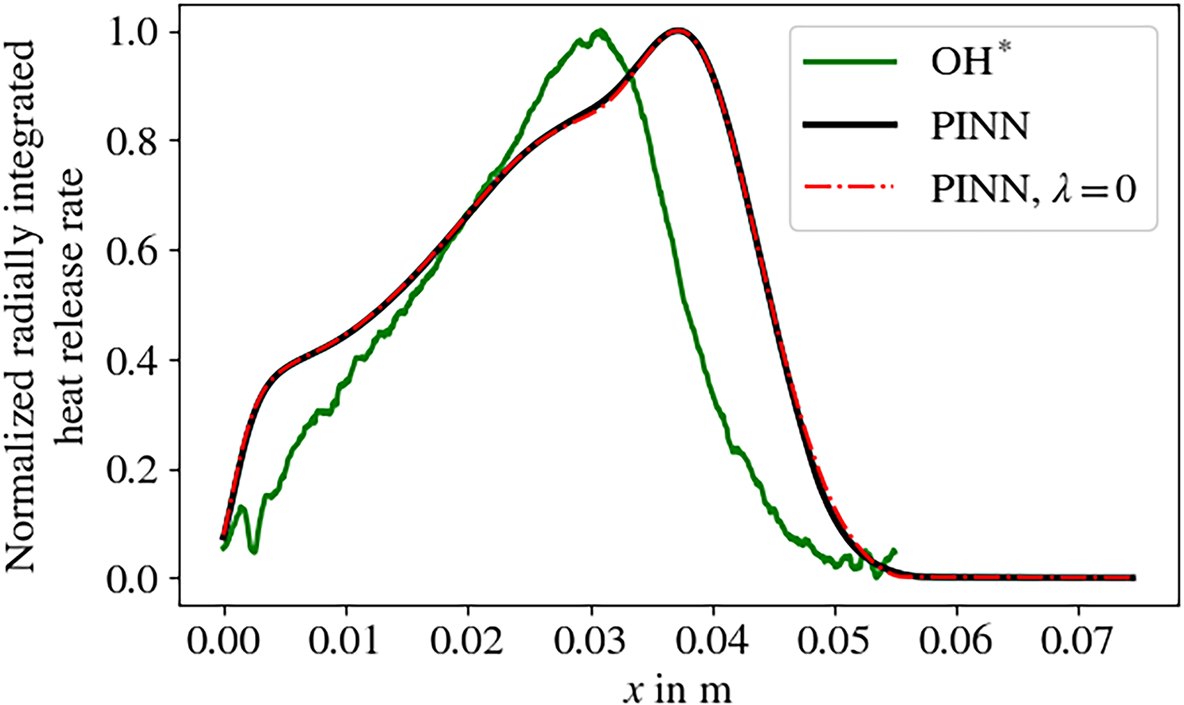A persistent increase of heat release rate along the $x$ -axis is visible with the maximum occurring between 0.03 and 0.04 m, after which the rate drops rapidly. As also observed in Figure 6, the PINN-based heat release rate is more pronounced near the anchoring point, and the flame extends slightly further downstream. Integrating the PINN-derived heat release rate along the axial direction yields a global heat release of 1.45 kW. Given that the combustor operated at a thermal power of 1.53 kW, this represents a very good approximation.

Figure 7.

Radially integrated heat release rate.

To further investigate the PINN assimilation results, the heat release field was recomputed for $λ = 0$ , effectively neglecting heat conduction, see equation (3). The corresponding radially integrated profile is shown as the dashed-dotted red line in Figure 7. Furthermore, Figure 8 shows radial profiles of heat release rate obtained with and without heat conduction in comparison to OH* profiles. Both figures indicate a minor influence of the conduction term on the identified heat release rate field. These results underscore the smoothing effect of a coarse PIV resolution in the assimilated fields, as observed above for density and temperature. It is well established that a significant share of heat fluxes in a laminar flame are generated through conduction.³⁵ Setting $λ = 0$ neglects these fluxes in the estimation of heat release, which should lead to a significant change in the identified flame structure. For reference, the distribution of heat release rate and the contributing terms from equation (3) for a one-dimensional flame simulated with Cantera are shown in Figure 13 in the Appendix, showing this substantial influence. However, the profiles shown in Figure 8 only indicate a minor shift of the identified heat release field due to conduction and the effect is significantly smaller than expected for a laminar flame. This is likely due to the fact that the influence of heat conduction is primarily determined by the Laplacian of the temperature field, whose contribution diminishes as gradients and second-order derivatives are smoothed.

Figure 8.

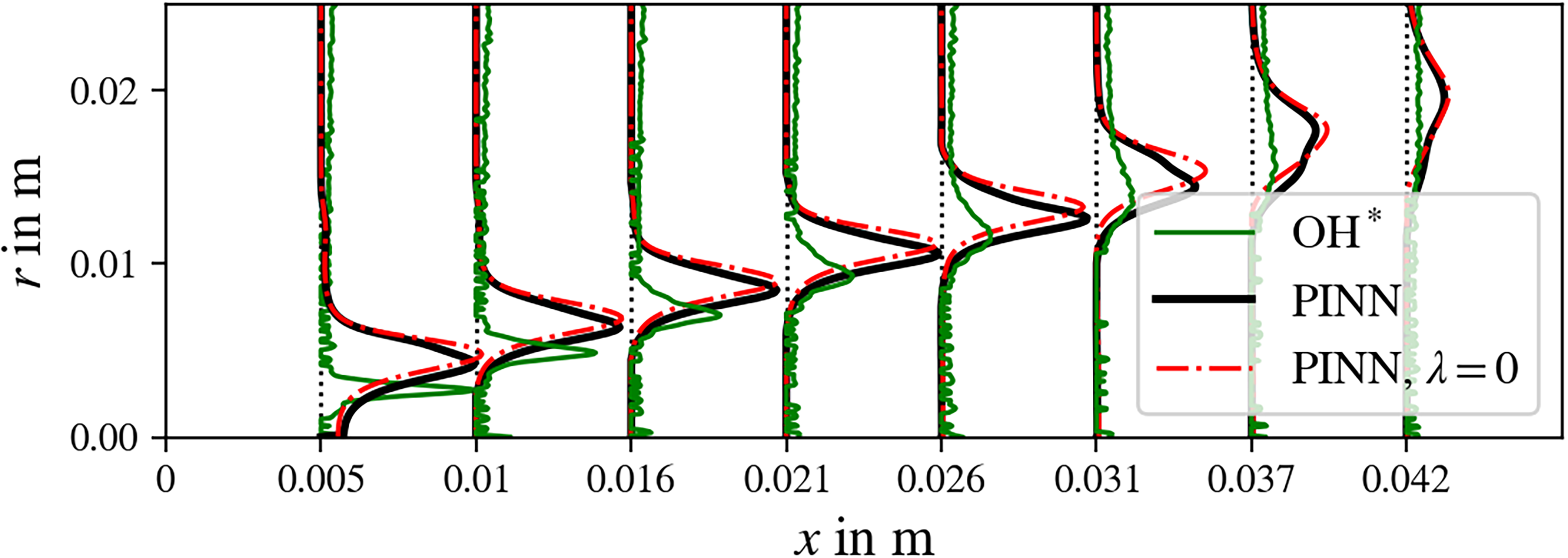
Radial profiles of normalized heat release rate from OH* chemiluminescence and from PINN predictions with and without heat conduction in the temperature equation.

In addition to the smoothed gradients resulting from the coarse PIV grid, the formulation of the cost function may contribute to an underestimation of the influence of the heat conduction term. The PINN cost function is limited to the continuity equation, which only contains first-order derivatives. Higher higher-order derivatives are thus not explicitly considered. The training therefore enforces an accurate representation of the data and first-order derivatives, but does not constrain higher-order derivatives to the same extent. Including, for example, momentum balances or derivatives of the continuity equation could improve the training in this respect.

The limited influence of heat conduction observed here means that the assimilated flame shape is primarily determined by the convection term in the energy equation. Although the total thermal power value from the experiments has been closely reproduced, it can thus be concluded that assimilation of the heat release field from sparse PIV data using the continuity and energy equations yields only qualitative results. The results show that the overall flame shape can be captured but not all underlying physical mechanisms are resolved. Improved accuracy may require either higher-resolution velocity fields or a more advanced assimilation approach.

Assimilation insights

To gain deeper insight into the assimilation process, we evaluate the contributing terms to the physics loss as proposed by Klopsch et al.³⁴ The continuity equation based on the trained network parameters can be formulated as follows:

\nabla \cdot u_{α *} + u_{α *} \cdot \frac{\nabla ρ_{α *}}{ρ_{α *}} = e_{α *}

(9)

Here, the first term represents the divergence of the velocity field, the second accounts for density variation, and

e_{α *}

is the residual. The velocity divergence is determined by the velocity field, for which training data are available that are well approximated by the PINN (see Figure 5). The second term includes the velocity and the inferred density field.

Figure 9 shows the absolute values of the three terms in equation (9). All fields are non-dimensionalized using the nozzle radius and the bulk velocity of the fresh gas within the nozzle. The top panel displays the velocity divergence. As expected, high values occur in the flame region, where an abrupt temperature increase leads to a density drop and thus flow acceleration. The middle panel shows the second term, illustrating that the PINN assimilates a density field with a corresponding gradient that compensates for the velocity divergence. As a result, the two terms balance, as evidenced by the small residual shown in the bottom panel. This demonstrates that the PINN successfully identifies the region of flow acceleration in the reaction zone from the velocity data and infers a physically consistent density field.

Figure 9.

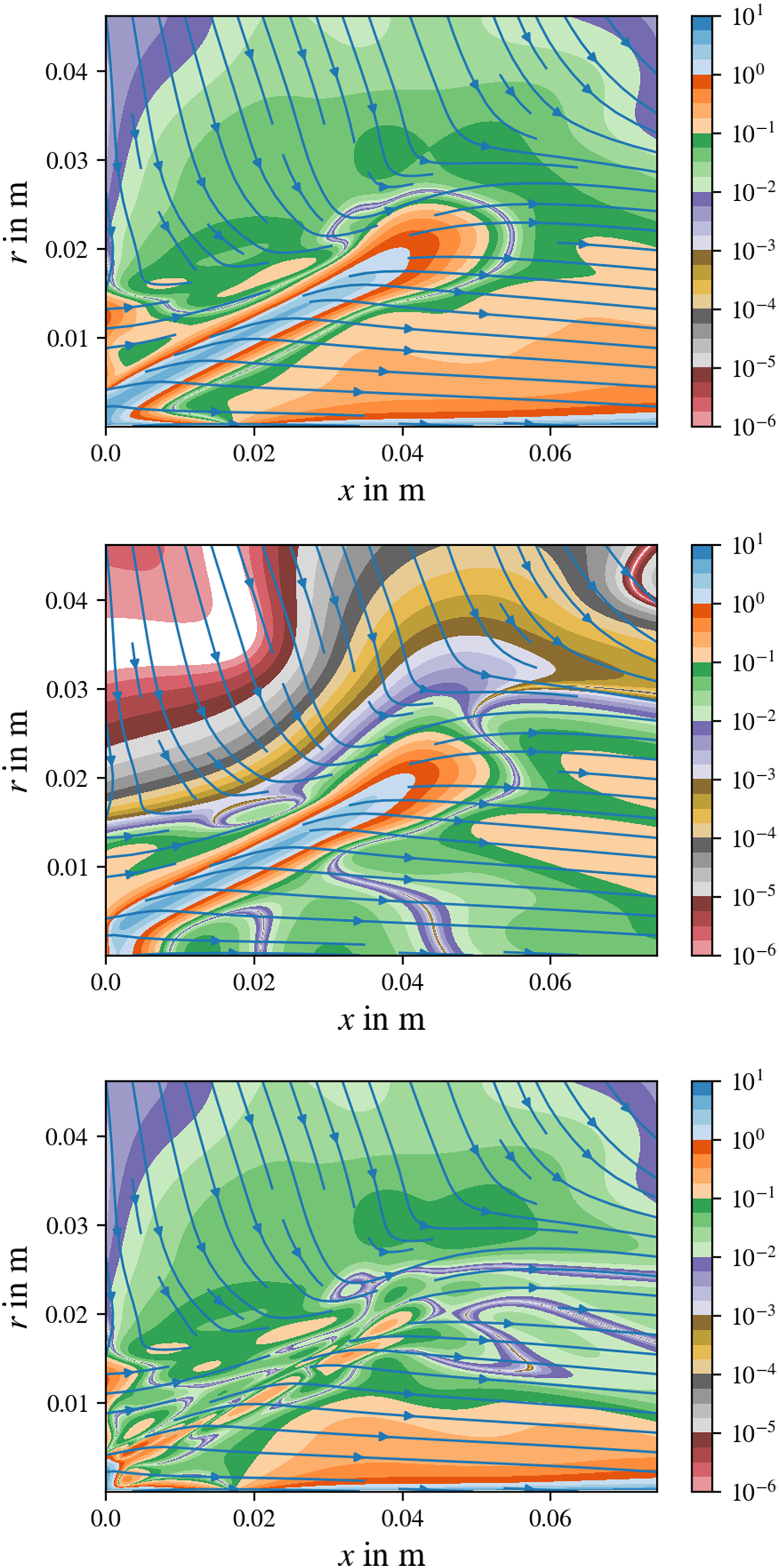
From top to bottom the absolute value of the three terms in equation (9): $| \nabla \cdot u_{α *} |$ , $| u_{α *} \cdot \nabla ρ_{α *} / ρ_{α *} |$ , and $| e_{α *} |$ .

A small region with residuals on the order of $10^{0}$ remains visible just downstream of the centerbody, close to the axis (see bottom panel). This region proved challenging for several reasons. It is located near the domain boundary, where PIV measurements are often unreliable. Moreover, it is bounded upstream by the centerbody and downstream by the flame anchoring point. The sparse PIV data likely fail to adequately resolve the complex flow structures present in this small area. The assimilation of the flame here proved to be particularly sensitive to the network architecture and training process.

The top panel in Figure 9 further reveals non-negligible velocity divergence outside the flame region, with values in the order of $10^{- 1}$ (green). In these areas, the observed divergence is more likely attributable to imperfections in the experimental conditions than due to an influence of the flame. Although the flow is assumed to be axisymmetric, the measured velocity field exhibits a small transverse component, likely caused by the laboratory exhaust system, which violates the axisymmetry assumption. Similarly, high residuals are visible along the axis in the downstream region in the top panel of Figure 9. Here, the velocity profiles do not comply with an axisymmetric flow, as evident from the radial velocity component being only approximately zero on the axis, see Figure 5. As the flow is expected to be divergence-free in these regions, the observed elevated residuals can be attributed to overfitting to the training data, which is a consequence of treating the velocity field as ground truth through high weighting in the loss function. Such artifacts can introduce an error in the inferred density fields as these are assimilated to comply with the velocity data.

In the case shown, these imperfections in the velocity measurements do not significantly impact the resulting density field. The identified critical regions in the top panel remain associated with elevated residuals of the continuity equation, as apparent in the bottom panel of Figure 9, and are thus not compensated by the inferred density field. However, increasing the network size and the number of trainable parameters, along with extended training, can lead to the transfer of this artifact into the inferred density field. This can result in identification of heat release away from the core flame region, which for a laminar flame is non-physical. Such behavior is a natural consequence of treating the velocity data effectively as ground truth and assimilating the density accordingly. To prevent these types of errors, the model setup is constrained, which is achieved by using a comparatively small network size. The presented results are robust with respect to small changes in the network architecture. However, when increasing the number of trainable parameters by one order of magnitude, the inferred density field degrades (not shown), as the residuals in the discussed regions are balanced by an unphysical density field.

Unsteady flow assimilation

Next, we shift the focus to the unsteady cases. Our main interest lies in the flame dynamics, quantified as the volume-integrated heat release rate oscillations. Typically, interest lies in the flame response in terms of the FTF. It quantifies the relative global heat release rate oscillation in relation to relative fluctuations of a characteristic forcing velocity. Such a characteristic velocity can be determined from both the PIV data and the PINN-assimilated velocity fields as

U (t) = \frac{1}{V_{r}} \int_{V_{r}} u_{x} (x, r, θ, t) d V

(10)

where

u_{x}

denotes the phase-averaged axial velocity component and

V_{r}

denotes a small inlet volume bounded by

x \in [5 mm, 7 mm]

r \in [9 mm, 13 mm]

, and

θ \in [0, 2 π]

, shown in red in the top panel in Figure 5. This volume lies within the expanding flow downstream of the nozzle exit. It is close to the nozzle but sufficiently far from the upstream boundary and the centerbody to avoid regions where PIV vectors are corrupted by boundary effects. From the volume-integrated instantaneous field, the fluctuating component can be obtained by subtracting the temporal mean,

U^{'} = U - \bar{U}

, where the prime and the bar denote the fluctuating and time-averaged quantities, respectively. The fields are assumed to be axisymmetric.

The relative global heat release rate is directly derived from the photomultiplier data by normalizing the signal with its mean value. To compute it from the PINN-assimilated heat release rate distribution, the global heat release rate is obtained by integrating the inferred distribution over the volume of the entire assimilation domain $V_{d}$ ,

Q (t) = \int_{V_{d}} q (x, r, θ, t) d V

(11)

where

q

is determined from the energy equation, see equation (3). Subtracting the temporal mean from

Q

yields the global fluctuating heat release rate

Q^{'}

Figure 10 presents the temporal evolution of the measured and PINN-assimilated velocity and heat release rate fluctuations over one period for forcing frequencies of 19, 47, 91, and 137 Hz. For the lower frequencies (19 and 47 Hz), the results are based on $N_{t} = 24$ discrete phase angles, while for the higher frequencies (91 and 137 Hz), $N_{t} = 48$ are used. The velocity fluctuation is normalized by the bulk velocity, and the heat release rate fluctuation by its mean value. The PINN reproduces the phase evolution of both quantities with high accuracy. For the velocity fluctuation, this agreement is expected, as velocity data were used for training. Notably, the PINN also captures the global heat release rate fluctuation with similar fidelity, with both phase and amplitude closely matching the OH* chemiluminescence measurements. The best agreement is observed at 19 Hz, with a slight degradation at higher frequencies, likely due to the shorter wavelengths and increased gradient magnitudes of the flow structures, which are more challenging to approximate. Additionally, the fluctuation amplitude in the heat release rate decreases with frequency, so that weaker fluctuations need to be identified by the PINN. At 47 Hz, a slight phase offset can be observed between the assimilated global heat release rate fluctuation and the photomultiplier signal. This is likely attributed to uncertainties in the assimilation procedure, such as the underestimated influence of heat conduction, an overestimated flame length as observed for the steady case, or a mismatch with the applied boundary conditions. At the highest forcing frequency of 137 Hz, the excitation is insufficient to produce a clear flame response. This is reflected in the measured phase-averaged OH* signal, which appears noisy and lacks a harmonic structure. While the PINN reproduces the noise amplitude with reasonable accuracy, it represents the integrated heat release response as a long-wavelength harmonic. This behavior results from the temporal coordinate embedding, which constrains the predicted velocity and density fields to satisfy the periodicity imposed by the forcing.

Figure 10.

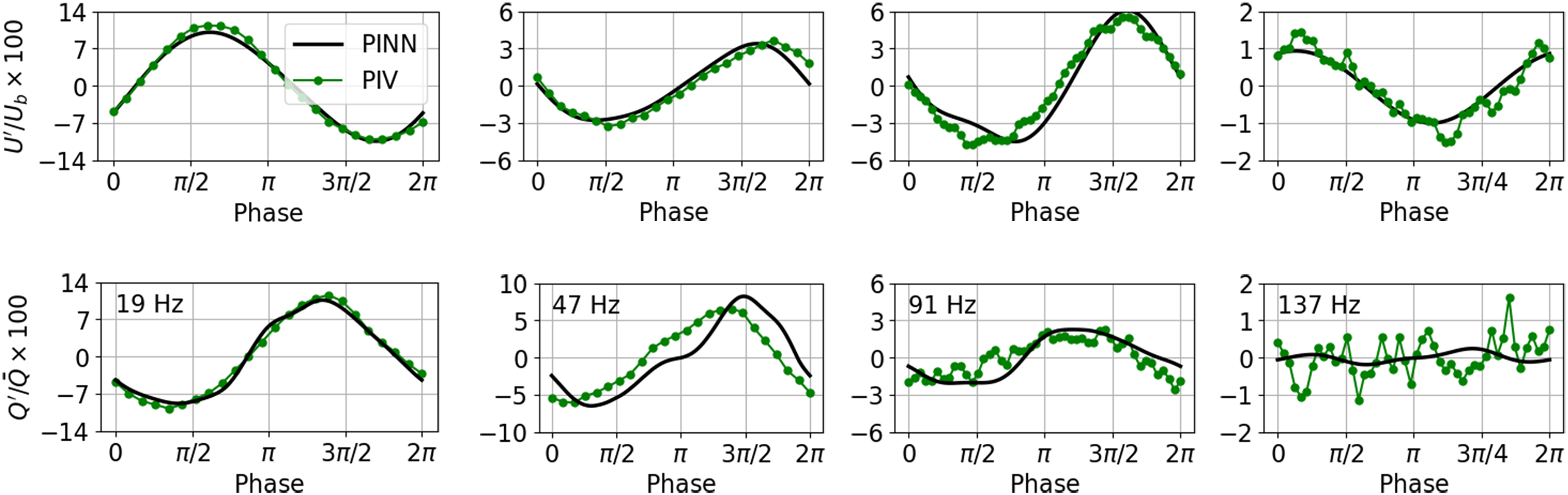
Normalized, phase-averaged characteristic velocity (top), and global heat release rate oscillation (bottom) for three forcing frequencies: 19, 47, 91, and 137 Hz (left to right). Black lines indicate the measured values; green lines indicate PINN-assimilated quantities.

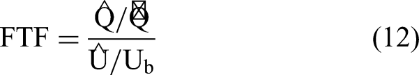
From the characteristic velocity fluctuation and the global heat release rate fluctuation, the FTF can be determined as follows:

FTF = \frac{\hat{Q} / \bar{Q}}{\hat{U} / U_{b}}

(12)

where the hat symbol denotes the Fourier coefficient at the excitation frequency. The complex FTFs for all six forcing frequencies are shown in Figure 11, with measured values indicated by green markers. These are calculated from

N_{t} = 24

phase angles but change only marginally with the number of bins. For the highest frequency (137 Hz), the measured FTF gain is close to zero, rendering the phase undefined. As a reference, we plot the phase of

\exp (- i ω τ_{c})

, with

τ_{c} = L_{f} / U_{b}

, which represents the phase lag between the nozzle exit and the flame tip for disturbances convected at the bulk flow velocity. The flame length,

L_{f}

, is approximated from Figure 6 to be

0.03

m and

ω

denotes the angular frequency. Approximating the flame response with a simple time lag model is a common approach for predicting combustion instabilities.²

Figure 11.

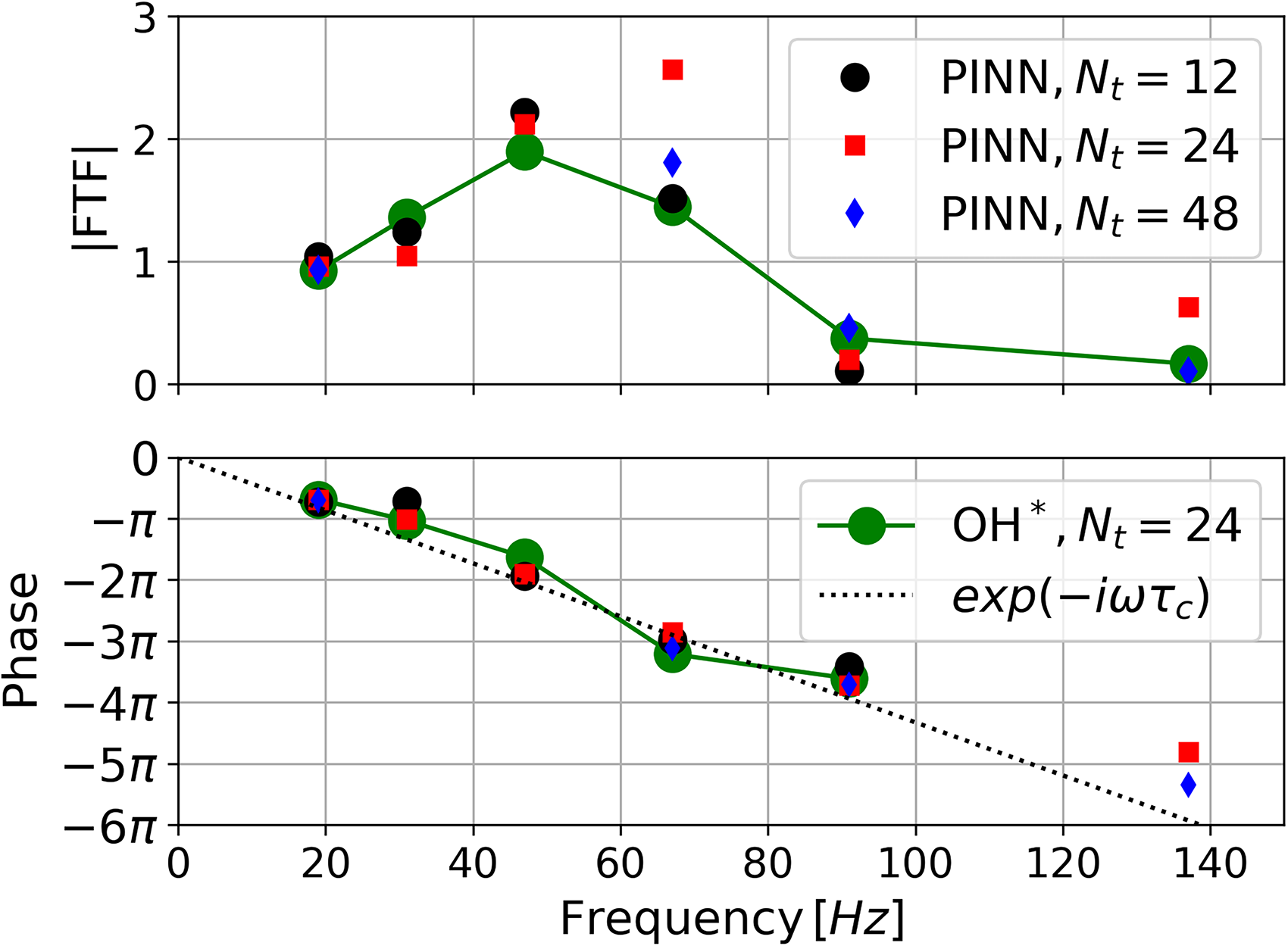
Flame transfer function at six forcing frequencies, determined from the characteristic velocity fluctuation and the OH* photomultiplier data (green), as well as from the PINN-assimilated velocity and heat release rate fluctuations. PINN-assimilated results are shown for phase averages with $N_{t} = 12$ (black), 24 (red), and 48 (blue) bins used as training data.

PINN-assimilated results are shown by black, red, and blue markers corresponding to training on phase averages with $N_{t} = 12$ , 24, and 48 bins, respectively. We note that not every combination of forcing frequency and number of phase bins has been assimilated. As anticipated from Figure 10, the PINN reproduces the measured FTF with reasonable accuracy, with both amplitude and phase trends well captured by the assimilated solution. For most forcing frequencies, the temporal resolution of the training data (i.e. the number of phase bins) has only a minor influence on the results. At the two highest forcing frequencies, 91 and 137 Hz, a higher temporal resolution yields a slight improvement in accuracy. In contrast, at 67 Hz a pronounced dependence on the temporal resolution is observed: the best agreement is obtained with $N_{t} = 12$ , while increasing the number of phase bins ( $N_{t} = 24$ , 48)—and thus the amount of training data—leads to degraded results. At this frequency, the assimilation generally proved challenging, also when other forcing amplitudes were tested (not shown). A possible explanation is that, at this intermediate frequency, the flame still exhibits a relatively strong response while the shear-layer structures are already shorter in wavelength. This combination suggests a more complex flow–flame interaction, which may be more difficult for the PINN to capture, particularly given the sparse spatial resolution of the PIV data. However, this explanation remains speculative, as no spatially resolved OH* measurements are available for the forced cases, which would capture the flow–flame interaction.

Besides the difficulty encountered at the intermediate frequency of 67 Hz, the overall agreement is very good. Small deviations can be observed, but given that the PINN is trained solely on PIV data from which it infers the heat release dynamics, the results are highly encouraging. This demonstrates that PINNs provide a promising framework for extracting flame dynamics from velocity fields.

Flame–flow interaction

The assimilation not only provides the global heat release rate fluctuations but also enables a more detailed investigation of the flow–flame interaction, as the PINN-assimilated solution yields the heat release rate as a function of space and time. Figure 12 presents instantaneous velocity fields (streamlines), vorticity fields (contours), and heat release rate isolines at 60% of their respective maximum values for four phase angles at two forcing frequencies: 19 Hz (left) and 47 Hz (right). All results presented are obtained from PINN approximations trained on 24-bin phase-averaged data.

Figure 12.

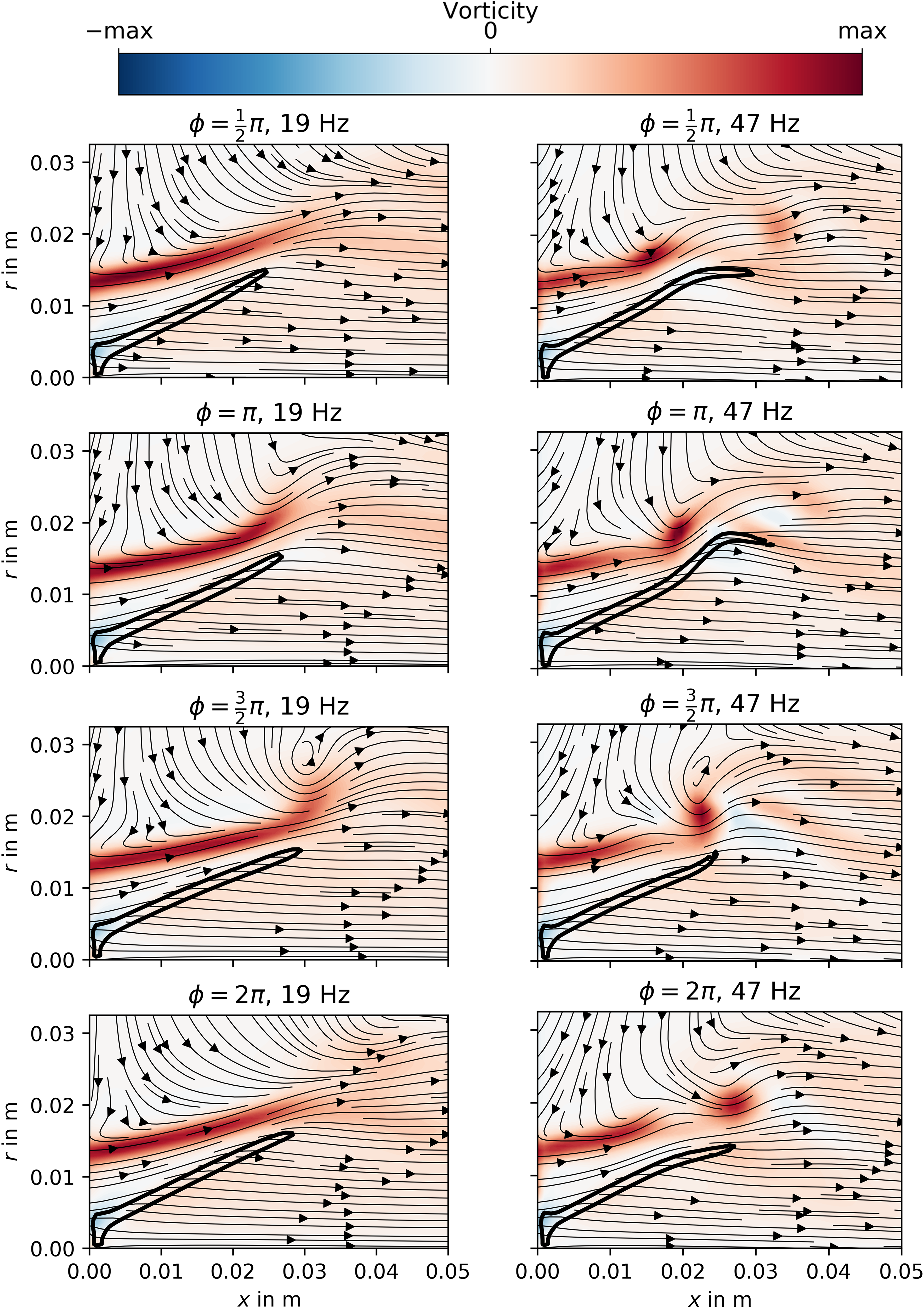
Instantaneous velocity field (streamlines), vorticity contours, and heat release rate isoline at 60% of the respective maximum value for two forcing frequencies: 19 Hz (left) and 47 Hz (right). Four phase angles are shown for each frequency. All results are obtained from the PINN-assimilated fields.

For the low forcing frequency of 19 Hz (left panels), a large persistent shear layer is observed as an elongated region of high vorticity. As the phase progresses, the shear layer first bends away from the axis and subsequently returns toward it. This flapping motion is induced by a large axissymmetric vortex generated by the acoustic forcing, which convects along the shear layer. The vortex initially displaces the flame toward larger radii, increasing the global heat release rate (see Figure 10 at a phase of $π$ and $3 / 2 π$ ), and later pushes the flame closer to the axis as the vortex detaches from the shear layer, reducing the global heat release rate.

At the higher forcing frequency of 47 Hz (right panels), a different behavior is observed. The shear layer is considerably shorter, and the rolling motion is more pronounced due to the decreased wavelength of the vortex forming within it. As the vortex convects downstream, it first displaces the flame toward larger radii and subsequently pushes it back toward the axis as it passes over the flame tip. In contrast to the lower-frequency case, the flame surface follows the vortex motion more closely, resulting in stronger flame roll-up and an increased global flame response, which manifests as a higher gain in the FTF. It is noted that due to the cylindrical coordinates, the volume contribution is largest at large radii, explaining the high gain values associated with this forcing frequency.

These results demonstrate that the PINN-assimilated fields provide valuable insight into the coupling between hydrodynamic structures, formed in the shear layer by acoustic forcing, and the resulting flame dynamics.

Conclusions

In this study, we present a data assimilation methodology based on PINNs that enables the estimation of heat release rate fields from PIV measurements. The approach is built on approximating the measured velocity field using a PINN while enforcing the continuity equation with variable density during training. This allows the network to infer the underlying density field directly from the velocity data. After training, the continuous and differentiable nature of neural networks is exploited to compute the temperature and heat release rate fields using the ideal gas law and an energy equation, respectively. As a result, the PINN framework provides a physically consistent estimate of the density, temperature, and heat release rate. The method is demonstrated using data from a laminar V-flame, showing good agreement in both steady and acoustically excited cases. For the steady case, the identified heat release fields are validated against experimental observations of the spatial distribution, while under acoustic excitation, the validation is performed against time-resolved global heat release values.

A detailed analysis of the results shows that the PINN infers the heat release distribution primarily from the convection term in the energy equation, which is determined through the available velocity training data and the continuity equation during network training. Consequently, the present approach yields only a qualitative representation of the heat release distribution. Heat conduction effects, which are known to play an important role in laminar flames, are not captured, likely due to the limited spatial resolution of the measured velocity fields and the resulting effective smoothing of spatial gradients. Nevertheless, the convection-based estimate provides a reasonable representation of the flame shape, the global heat release rate and, most importantly, offers valuable insight into flow–flame interactions. This capability enables the extraction of flame transfer functions with good accuracy based solely on phase-averaged velocity measurements.

Future work will focus on extending the methodology to infer not only the heat release field but also the fuel species distribution, thereby providing the input fields required for resolvent or linear stability analyses. Additionally, the approach will be adapted for application to turbulent flames as they are used in industrial combustors.

Footnotes

Acknowledgements

Funded by the Deutsche Forschungsgemeinschaft (DFG, German Research Foundation) – 506170981. This work was supported by a postdoc fellowship of the German Academic Exchange Service (DAAD). We would like to thank K. J. Lindenberg and C. Hausherr for conducting the experimental measurements and providing related information. We also thank Roman Klopsch for maintaining our PINN code. Generative artificial-intelligence tools, specifically ChatGPT and DeepL, were used exclusively for linguistic refinement.

ORCID iDs

Jakob Georg Raimund von Saldern

Johann Moritz Reumschüssel

Thomas Ludwig Kaiser

Kilian Oberleithner

Funding

The authors received no financial support for the research, authorship and/or publication of this article.

Declaration of conflicting interests

The authors declare no potential conflicts of interest with respect to research, authorship, and publication of this article.

Appendix

To examine the contributions of the heat fluxes appearing in the enthalpy equation (equation (3)) to the heat release rate distribution, Figure 13 shows the results of a one-dimensional simulation of a freely propagating flame. The inflow conditions were adapted to match the experiments, and the simulation was conducted using Cantera with the GRI3.0 mechanism. Following equation (3), the terms for heat convection and conduction are calculated from the density and temperature distributions. The plot shows that convection (red line) results in a positive flux, meaning in the direction of flow. Heat conduction (blue line) results in a heat flux from the reaction zone in both directions. Both contributions are comparable in magnitude. The heat release rate (black line) is equal to the sum of the fluxes and shows a sharp peak. If the heat conduction term is neglected in this calculation, the estimated heat release rate becomes equal to the convection term only. In this case, the flame appears wider with less pronounced gradients, and is located further upstream. This effect is also observed when postprocessing the assimilated fields, indicating an underestimation of the conduction term.

References

Poinsot

Veynante

. Theoretical and numerical combustion. RT Edwards Inc 2005; 1: 522.

Lieuwen

Yang

. Combustion instabilities in gas turbine engines: operational experience, fundamental mechanisms, and modeling (Progress in Astronautics and Aeronautics). 2005. ISBN 156347669X. DOI: 10.2514/4.866807.

Poinsot

Trouve

Veynante

, et al. Vortex-driven acoustically coupled combustion instabilities. J Fluid Mech 1987; 177: 265–292.

Keller

. Thermoacoustic oscillations in combustion chambers of gas turbines. AIAA J 1995; 33: 2280–2287.

Morgans

Yang

. Thermoacoustic instability in combustors. Annu Rev Fluid Mech 2024; 57: 9–33.

Selle

Lartigue

Poinsot

, et al. Compressible large eddy simulation of turbulent combustion in complex geometry on unstructured meshes. Combust Flame 2004; 137: 489–505.

Dowling

. The calculation of thermoacoustic oscillations. J Sound Vib 1995; 180: 557–581.

Kopitz

Huber

Sattelmayer

, et al. Thermoacoustic stability analysis of an annular combustion chamber with acoustic low order modeling and validation against experiment. pp.583–593. DOI: 10.1115/GT2005-68797.

von Saldern

JGR

Orchini

Moeck

. Analysis of thermoacoustic modes in can-annular combustors using effective bloch-type boundary conditions. J Eng Gas Turbine Power 2021; 143: 071019.

10.

Sattelmayer

Polifke

. A novel method for the computation of the linear stability of combustors. Combust Sci Technol 2003; 175: 477–497.

11.

Merk

Buschmann

Moeck

, et al. The nonlinear thermoacoustic eigenvalue problem and its rational approximations: assessment of solution strategies. J Eng Gas Turbine Power 2022; 145: 021028.

12.

Reumschüssel

Kroll

von Saldern

JGR

, et al. Flame transfer function shaping for robust thermoacoustic systems: application to a kinematic flame model. Int J Spray Combust Dyn 2024; 16: 48–59.

13.

Orchini

Cronqvist

von Saldern

JGR

, et al. Tracking of acoustic and intrinsic modes for thermoacoustic systems with a general flame model. Combust Flame 2025; 275: 113998.

14.

Paschereit

Schuermans

Polifke

, et al. Measurement of transfer matrices and source terms of premixed flames. J Eng Gas Turbine Power 2002; 124: 239–247.

15.

Schuermans

Guethe

Mohr

. Optical transfer function measurements for technically premixed flames. J Eng Gas Turbine Power 2010; 132: 081501.

16.

Raissi

Perdikaris

Karniadakis

. Physics-informed neural networks: a deep learning framework for solving forward and inverse problems involving nonlinear partial differential equations. J Comput Phys 2019; 378: 686–707.

17.

Raissi

Yazdani

Karniadakis

. Hidden fluid mechanics: learning velocity and pressure fields from flow visualizations. Science 2020; 367: 1026–1030.

18.

Zhang

Wang

. Explore missing flow dynamics by physics-informed deep learning: the parameterized governing systems. Phys Fluids 2021; 33: 095116.

19.

Cai

Mao

Wang

, et al. Physics-informed neural networks (PINNs) for fluid mechanics: a review. Acta Mech Sinica 2021; 37: 1727–1738.

20.

Eivazi

Tahani

Schlatter

, et al. Physics-informed neural networks for solving Reynolds-averaged Navier Stokes equations. Phys Fluids 2022; 34: 075117.

21.

Wang

Liu

Wang

. Dense velocity reconstruction from particle image velocimetry/particle tracking velocimetry using a physics-informed neural network. Phys Fluids 2022; 34: 017116.

22.

von Saldern

JGR

Reumschüssel

Kaiser

, et al. Mean flow data assimilation based on physics-informed neural networks. Phys Fluids 2022; 34: 115129.

23.

Steinfurth

Weiss

. Assimilating experimental data of a mean three-dimensional separated flow using physics-informed neural networks. Phys Fluids 2024; 36: 015131.

24.

Hasanuzzaman

Eivazi

Merbold

, et al. Enhancement of PIV measurements via physics-informed neural networks. Meas Sci Technol 2023; 34: 044002.

25.

Villié

Schmitter

von Saldern

JGR

, et al. Physics-informed neural networks for enhancing medical flow magnetic resonance imaging: artifact correction and mean pressure and Reynolds stresses assimilation. Phys Fluids 2025; 37: 025194.

26.

Taassob

Ranade

Echekki

. Physics-informed neural networks for turbulent combustion: toward extracting more statistics and closure from point multiscalar measurements. Energy Fuels 2023; 37: 17484–17498.

27.

Taassob

Kumar

Gitushi

, et al. A PINN-deeponet framework for extracting turbulent combustion closure from multiscalar measurements. Comput Methods Appl Mech Eng 2024; 429: 117163.

28.

von Saldern

JGR

Beuth

Reumschüssel

, et al. Low-frequency streaky structures in turbulent hydrogen jet flames. Combust Flame 2025; 278: 114231.

29.

Yadav

Casel

Ghani

. Rf-pinns: reactive flow physics-informed neural networks for field reconstruction of laminar and turbulent flames using sparse data. J Comput Phys 2025; 524: 113698.

30.

Tathawadekar

Silva

Sitte

, et al. Physical quantities reconstruction in reacting flows with deep learning. In: INTER-NOISE and NOISE-CON congress and conference proceedings, Vol. 265, pp.1645–1656. Institute of Noise Control Engineering. DOI: 10.3397/IN_2022_0235.

31.

Roehle

Schodl

Voigt

, et al. Recent developments and applications of quantitative laser light sheet measuring techniques in turbomachinery components. Meas Sci Technol 2000; 11: 1023.

32.

Terhaar

Paschereit

. High-speed PIV investigation of coherent structures in a swirl-stabilized combustor operating at dry and steam-diluted conditions. In: 16th International symposium on applications of laser techniques to fluid mechanics.

33.

Oberleithner

Terhaar

Rukes

, et al. Why nonuniform density suppresses the precessing vortex core. J Eng Gas Turbine Power 2013; 135: 121506.

34.

Klopsch

Fuchs

Rigas

, et al. Enabling resolvent analysis through assimilation of experimental mean flows with physics-informed neural networks: a case study on the Boeing Gaussian bump. American Institute of Aeronautics and Astronautics. ISBN 978-1-62410-738-2. DOI: 10.2514/6.2025-3604.

35.

Turns

. An Introduction to Combustion. Vol. 287. New York: McGraw-Hill, 1996.