



Abstract
One of the challenges for software developers in incremental development methodologies is the issue of the next release problem. In this article, for the first time, this problem will be solved with three goals namely cost, satisfaction, and dissatisfaction. It also has several types of constraints. These three conflicting goals and different constraints make it extremely difficult to choose the optimal subset for product manufacturers. Wrong choices will lead to increased customer dissatisfaction and reduced product sales. To help make smart and error-free choices, we introduce two algorithms. These algorithms determine the merit of the requirements using the fuzzy inference system and then make the choices based on the type of threshold value constraint. We also introduce and implement the constraint of the impact of dissatisfaction on requirements. To conduct the experiments, the proposed algorithm has been compared with the algorithms FMACRO, IBPSO and Kmeans. In all experiments, the solutions resulted from the proposed algorithms had higher quality than the other three algorithms. These results show that choosing the proposed algorithms can provide more satisfaction to customers, reducing their dissatisfaction and lowering product prices. The most important advantages of the proposed algorithms are its scalability and linear order time complexity.
Keywords
Introduction
There are several approaches to developing software. One of the most popular methods for producing complex software is the incremental development method. In this approach, the software product will develop in several releases. The development team, at each release, faces a set of requirements for software development. Each software is produced for a specific purpose and use. The development team must implement the functional and non-functional requirements of the software. Customers and members of the development team propose the requirements (Pirozmand et al., 2021). Due to various constraints, it is not possible to develop all the proposed requirements in one release. In each release, the development team should select a subset of the proposed requirements that will provide the least production cost, maximum customer satisfaction, and the least amount of dissatisfaction.
Nayebi and Ruhe (2018) proposed the concept of Asymmetric Release Planning. The idea was that the development of a requirement in the next release may generate a satisfactory amount while the lack of its development will not cause any discontent. Or, conversely, the development of a requirement does not create any satisfaction, but the lack of it can cause great dissatisfaction. For example, not using the start button in the early version of Windows 8 caused a lot of dissatisfaction for users, while users would not have been satisfied if it was used like in previous versions of Windows. As explained, there are several conflicting objective functions, such as maximizing satisfaction, minimizing dissatisfaction and cost. There are also two general constraints to this problem. One of these is the intrinsic relationship between the requirements, and the other is the threshold value constraints imposed on the project. These conflicting goals and constraints make it impossible to empirically select the optimal subset, especially if the number of requirements is high. Experimental and traditional choices are always accompanied with human error. The result of these non-optimal choices is the increase of customer dissatisfaction and product sales reduction.
Choosing an optimal subset is a challenge that software engineers are always faced with in incremental development methods (Alrezaamiri et al., 2019). For this reason, a development team needs a smart tool for making the right decisions. There are several ways to solve the NRP problem. Some of these methods have been based on linear programming (Domínguez-Ríos et al., 2019). These methods find the exact solution of the problem at high run time. If the number of requirements is high, this method is not suitable because of the high run time. Due to the reduction in run time, heuristic and meta-heuristic approaches have received much attention (Del Sagrado et al., 2015). Some researchers weighted the goals and converted this to the single goal problem. Selection of appropriate coefficients has been one of the disadvantages of these methods reducing the quality of the results. Part of the research used multi-objective meta-algorithms. If the number of goals and constraints increases, the quality of the results of these algorithms will also decrease. In recent years, several research studies have used fuzzy logic to prioritize requirements. The results of these papers show that the use of fuzzy concepts can be a good way to decide and select requirements.
Our goal in this paper is to introduce an intelligence algorithm to select the best set of requirements for the development team, despite several conflicting goals and several different constraints. In this paper, we use the fuzzy inference system to select the optimal subset. That is, we determine the merit of any requirement by means of laws for development in the next release, and then select the optimal subset according to the constraints in the problem. Nayebi and Ruhe (2018) considered two goals of satisfaction and dissatisfaction in NRP for the first time. However, the cost target was not taken into account. Cost is one of the important factors in the success and popularity of a software. The high cost of a product leads to a lack of customer satisfaction and a reduction in the profits of the IT company. So, in addition to the goals of customer satisfaction and dissatisfaction, it is also necessary to consider the cost goal, because a product with maximum satisfaction and minimum dissatisfaction and a high cost may still not be welcomed by customers. In consideration of the three conflicting objectives, which are given equal importance, the NRP problem is formulated as a multi-criteria problem. The selection of requirements is made on the basis of merit-based decision-making for each requirement. The motivation underlying the presentation of this paper is to introduce a methodology that selects the optimal subset of requirements, taking into account all criteria and constraints, with the objective of achieving the highest levels of customer satisfaction and satisfaction cost, and the lowest levels of dissatisfaction cost.
The primary contributions of this study are outlined as follows:
In this study, the three objectives of enhancing customer satisfaction, mitigating customer dissatisfaction, and reducing product costs were evaluated collectively for the first time. The second step in the process involves the implementation of an algorithm, which serves to transform the obtained crisp values from the customer survey into triangular or trapezoidal numbers. In a departure from the previous studies, the constraint effect on satisfaction (EOS) between requirements has been defined and implemented for the first time. In the field of research, an algorithm has been presented for the purpose of selecting the optimal subset. This subset is intended to determine the precise amount of customer dissatisfaction that occurred prior to the commencement of development.
The remainder of the paper is organised as follows: Section 2 provides an exhaustive review of the pertinent literature, emphasising seminal contributions and research conducted by other scholars in this field. In Section 3, a comprehensive explanation of the proposed method and materials is presented, detailing the theoretical framework, methodologies, and the resources utilised in the approach. The fourth section of this study focuses on the experimental setup, wherein a series of tests and evaluations are conducted to assess the performance and effectiveness of the proposed method. The results of these experiments are analysed and discussed in detail to demonstrate the strengths and limitations of the approach. Finally, Section 5 concludes the paper by summarising the key findings, drawing conclusions from the research, and suggesting potential directions for future work in this area.
Literature Review
Many researches have been done by scholars to solve NRP. A number of papers have categorized the presented methods (Zhang et al., 2018; Ramirez et al., 2019). Most of the methods presented are based on metaheuristic or requirements prioritization. The first attempt to solve the NRP problem was made by Bagnall et al. (2001). In that paper, the two objectives of cost reduction and customer satisfaction were investigated. This article was introduced as the standard version of the NRP issue. Bagnall et al. (2001) used several local search algorithms and a linear programming-based algorithm.
Greer and Ruhe (2004) solved the NRP problem in 2004 using a genetic algorithm in a dynamic environment. They called the algorithm Evolve, which subsequently attracted researchers for using and improving the method in following years. Jiang et al. (2010) used the ACO and Hill climbing algorithm to solve the NRP problem (Jiang et al., 2010). The authors showed in their experiments that combining the two algorithms together yields better results than the independent implementation of either algorithm. Masadeh et al. (2018) used the gray wolf optimization algorithm for choosing the optimal subset to development in the next release.
Del Sagrado et al. (2015) used the ACS algorithm to solve the NRP problem. They defined three types of relationships between requirements that attracted the attention of future researchers. Chaves-González and Pérez-Toledano (2015) solved the NRP uses three different meta-heuristics. The authors used the differential evolution with Pareto tournament algorithm (Chaves-González & Pérez-Toledano, 2015), the artificial bee colony optimization algorithm (Chaves-Gonzalez et al., 2015a) and the teaching learning-based optimization with Pareto tournament algorithm (Chaves-González et al., 2015b).
Alrezaamiri et al. (2019) introduced a metaheuristic algorithm with the name of fuzzy multi-objective artificial chemical reaction optimization algorithm (FMACRO) for finding an optimal subset. The authors considered the two objectives of cost and satisfaction. Balogun et al. (2016) introduced a hybrid metaheuristic algorithm to solve the NRP problem. Their proposed algorithm is a combination of Variable Neighborhood Search and Tabu Search. Hamdy and Mohamed (2019) introduced the Greedy Binary Particle Swarm Optimization algorithm to solve this problem. They were able to introduce a better version of the algorithm than the standard version of the algorithm by making some modifications. Their changes included modification in generating initial particles and also updating the operation of the velocity and positioning vectors. These authors solved this problem as a single objective by weighting and normalizing the satisfaction and cost goals. Dukhan et al. (2022) presented a hybrid metaheuristic algorithm, which was designated HGABC. The proposed algorithm is a combination of the genetic algorithm and the artificial bee colony algorithm.
For the first time, Alrezaamiri et al. (2019) used a parallelization technique to solve the NRP. They achieved remarkable results by running several artificial bee colony algorithms in shared memory and combining non-dominated solutions. Mougouei and Powers (2021) introduced the Dependency-Aware Requirement Selection algorithm in 2020. The algorithm first identifies the dependencies between the requirements and their modeling. In the second step, it solves the problem using the integer linear programming model. If the number of the proposed requirements in the algorithm is high, this technique will take a long run time to execute. Del Sagrado and del Águila (2021) proposed a combination of the qualitative MoSCoW method and cluster analysis for requirements selection. MoSCoW is a qualitative technique for requirements prioritisation. It is based on the classification of requirements using plain English meanings of the prioritisation categories. The objective of clustering methods is to partition m observations into k clusters in such a way that observations in one cluster are more similar to each other than those in other clusters.
A number of studies have employed fuzzy inference systems to assess the severity of other issues, including the NRP problem. Pandey et al. employed a fuzzy analytic hierarchy process in paper (Pandey & Litoriya, 2021). The objective of this paper is to provide a process selection framework for engineers and managers seeking to identify the most appropriate methodology for developing software to run on desktop, mobile or web platforms. In their seminal paper, Koohathongsumrit and Meethom (2021) proposed a novel integrated framework combining fuzzy risk assessment, data envelopment analysis and multiple criteria decision-making approaches for route selection in multimodal transportation networks. The proposed framework assists in enhancing the predictability of risk in multimodal transportation networks and facilitates decision-making processes for selecting the most suitable alternative.
Ramzan et al. (2011) proposed the multi-level value-based requirements prioritization technique using fuzzy logic. Using this technique, the authors selected the requirements. Alrashoud and Abhari (2015) used a fuzzy inference engine to prioritize the requirements. They considered effort, risks and the value of requirements. Alrashoud and Abhari (2017) considered three objectives of risk, customer satisfaction, and resource availability to solve the NRP. They used ANFIS to create fuzzy laws and then solved the problem with a fuzzy inference system. Alrezaamiri et al. (2020a) solved the NRP by considering intense competition in the market and copying product ideas. To prevent copying of product ideas, they added the goal of reducing development time. The goal of reducing development time in large projects that use incremental development is very important. The authors solved the problem using a fuzzy inference system. Table 1 provides a concise summary of the methodologies, evaluation criteria, benefits and drawbacks associated with NRP solving algorithms.
Summarizes the Methods, Criteria, Advantages, and Disadvantages of NRP Solving Algorithms.
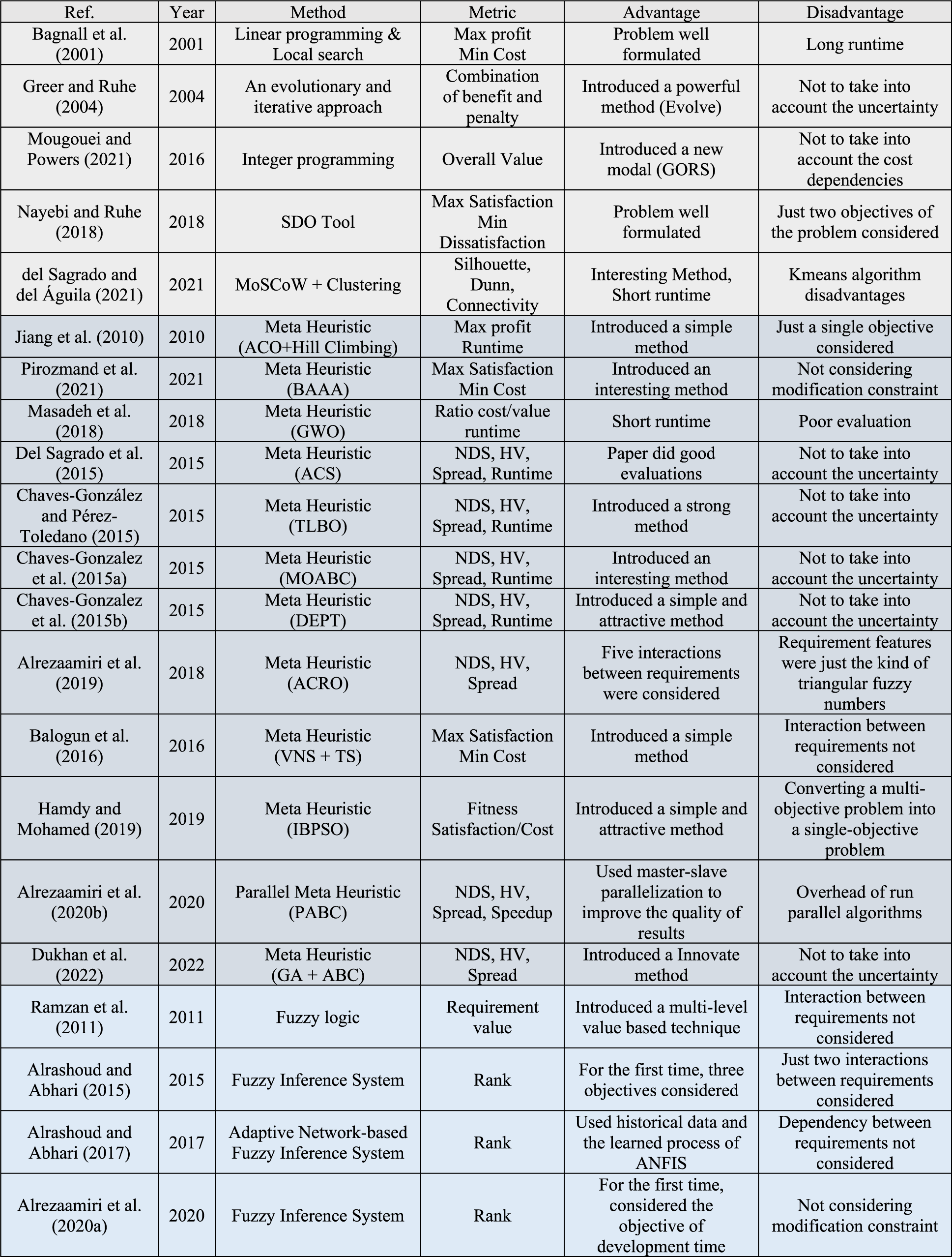
Summarizes the Methods, Criteria, Advantages, and Disadvantages of NRP Solving Algorithms.
In this section, we will first formulate the next release problem and, after defining the basic fuzzy operators, introduce the proposed method.
The Next Release Problem Formulation
In the NRP issue, prior to the development of each release, n requirements
Every requirement has an amount of development satisfaction, an amount of dissatisfaction with lack of development and an amount of cost for production. Satisfaction and dissatisfaction of each requirement is surveyed by customer and with sets of
In this problem, the goal is to find the best subset of the proposed requirements that provide the highest amount of satisfaction and the lowest amount of cost and dissatisfaction for customers and also does not violate the limitations defined in the issue.
There are two types of constraints, the relationship between the requirements and the threshold value. There are different types of relationship between requirements. del Sagrado divided the relationship between requirements into four classes (Del Sagrado et al., 2015).
Implication Combination Exclusion Modification. The implementation of requirement
Relationships between requirements are very common in software development. For example, an exclusion relationship between two requirements ri and rj means that it is not possible to develop both requirements in a single release, and the development team must choose at most one of them. The existence of these relationships makes it much more difficult to select the optimal subset.
Class IV of this type of constraints has been neglected in all past research, while having a huge impact on the results. Alrezaamiri et al. (2019) broken this class into two separate parts and introduced new definitions as follows.
Given the object of the dissatisfaction with the NRP problem, a new dependency will be created that we call the effect on the dissatisfaction and define it as follows:
The three constraints of effect on the cost, effect on the dissatisfaction and effect on the satisfaction along with the constraints of Implication, Combination, and Exclusion make the problem more realistic and more practical. We use all of these six types in implementation. The second general type of constraint is the threshold values for the project. These values are usually set by the development team. The amount of cost and satisfaction of the subset selected for development in the next release is calculated from the sum of the selected requirements. The amount of dissatisfaction is the sum of every single unselected requirement for development in the next release. The sum of these values should not violate the threshold value. Figure 1 shows the seven requirements. Requirements selected for development in the next release are shown in green, and requirements not selected are shown in red.
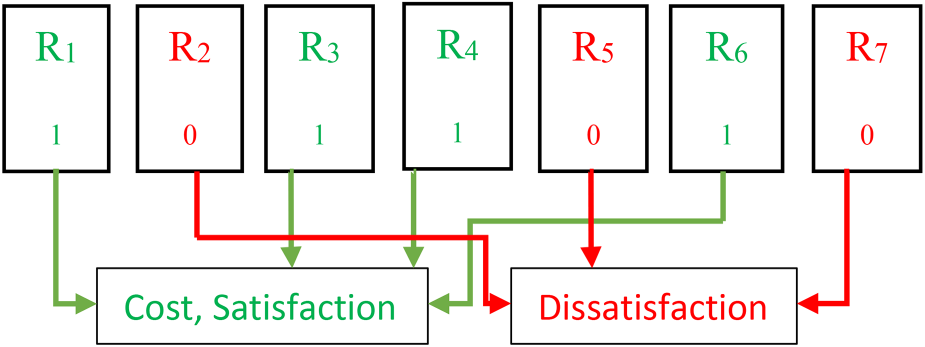
Selected and Unselected Requirements for Development in Next Release.
If the amount of 10% dissatisfaction threshold is set, that is, from the total set of proposed requirements, a subset that has the highest satisfaction and the least cost should be selected, and on the other hand, a subset that is not selected should have a dissatisfaction value of less than 10%. Or, as another example, if the amount of 85% cost threshold is considered, it means that a subset should be selected that provides the highest satisfaction at a cost of less than 85% and the unselected subset should have the least dissatisfaction for customers.
In this section, we describe fuzzy computational operators (Di Caprio et al., 2022; Ebrahimnejad et al., 2016).


A trapezoidal fuzzy number denoted by

a. Trapezoidal fuzzy number (−1, 0, 2, 4). b. Triangular Fuzzy Number (−2, 0, 2).
Summation of two trapezoidal numbers 
Summation of two triangular numbers 
Also, if we want to add a trapezoidal like 
If 
There are various methods for ranking trapezoidal fuzzy numbers such as 
If
In this section, we explain the proposed method with more details. The proposed algorithm is based on the use of a fuzzy inference system and greedy choices. In this method, the satisfaction and dissatisfaction of each requirement is obtained through a questionnaire from customers.
For example, k customer chooses a value between 0 and 10 as the amount of satisfaction with the development and a value as the dissatisfaction with the lack of development for each requirement. Because of the changing priorities of customers during implementation time, it is better to use uncertain numbers as parameters of each requirement instead of Crisp numbers. In our study, the decision to use fuzzy numbers is motivated by the inherent uncertainty and subjectivity in customer responses that is common in software development environments. As highlighted by Pressman (2005), customer priorities and requirements often change during the software development process due to various factors, including better understanding of needs, shifts in the business environment, changes in market conditions, and regulatory influences. These dynamic factors contribute to the ambiguity in the data, making fuzzy numbers a natural fit to accurately represent such uncertainties. To convert the questionnaire data into triangular or trapezoidal fuzzy numbers, we used a method commonly used in fuzzy decision making, where expert responses or customer ratings are interpreted as fuzzy sets. This allows us to represent the imprecision inherent in the responses. Triangular and trapezoidal fuzzy numbers were specifically chosen because they provide a straightforward representation of such ambiguity, with their parameters reflecting the range of possible values and the likelihood of a response within that range. In summary, the use of fuzzy numbers in this context not only addresses the flexibility required for customer preferences, but also improves the accuracy of the decision process by accounting for uncertainty in the data, as discussed by Pressman (2005).
The development team converts the values received from the k customers for each requirement based on Algorithm 1 to triangular or trapezoidal fuzzy numbers. If the standard deviation of the received data is less than a threshold value, these data are converted to triangular fuzzy numbers and otherwise converted to trapezoidal fuzzy numbers.
The reason for using these two types of fuzzy numbers in algorithm 1 is their simplicity, ease of interpretation, and widespread use in similar studies, ensuring both computational efficiency and practical applicability. Any other type of fuzzy number that can represent the transformation of a set of crisp numbers into a fuzzy number can also be considered and used. The algorithm is flexible and can accommodate alternative fuzzy representations depending on the specific needs or preferences of future studies. In our approach, Algorithm 1 is a heuristic method designed to transform a set of crisp numbers into fuzzy numbers. Triangular fuzzy numbers are used for crisp data that are less dispersed around the mean, while trapezoidal fuzzy numbers are used for data with greater dispersion. The standard deviation is the criterion we use to assess the distribution of the numbers around the mean. For the specific choice of the triangular fuzzy number (0, 2, 4), this was selected based on the standard deviation of the survey data, which indicated that the values were not widely spread out. As such, a triangular representation was appropriate for capturing the central tendency of the data with minimal fuzziness.
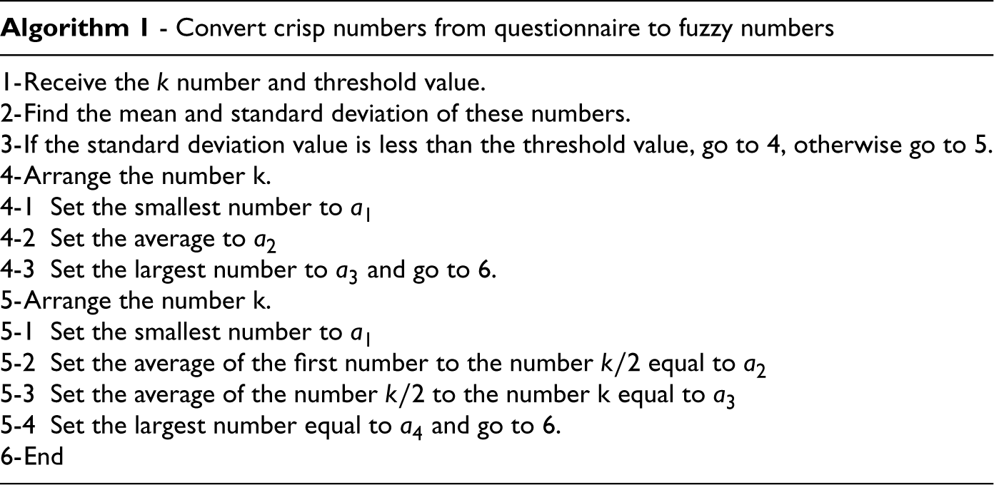
The threshold value is determined by the development team and should be selected according to the range of the amounts of the parameters within the questionnaire. If the standard deviation of the input numbers is less than the threshold value, it means that the numbers are around the mean and have less scatter. In this case, it is more appropriate to convert to triangular numbers.
However, if the standard deviation of the numbers is greater than the threshold, it means that the numbers are dispersed largely from the average, and it is more reasonable to convert to the trapezoidal numbers. In the following, we show the conversion of the extracted Crisp numbers from the questionnaire to fuzzy numbers with two examples, assuming a threshold value of 2.5.
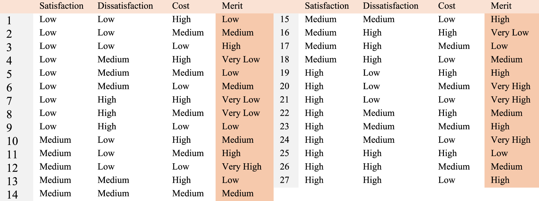
The cost of implementing each requirement is also determined by a fuzzy number, according to the experts. The fuzzy inference system has great power in solving decision problems. In this issue, for determining the merit of each requirement for development in the next release we use four fuzzy variables and Mamdani inference engine (Ye et al., 2024; Al-Nahhas et al., 2024). We define three input fuzzy variables for satisfaction, dissatisfaction, and implementation cost. Each of these input variables will have three high, medium, and low language variables. We also specify an output fuzzy variable to determine the merit of each requirement that has five language variables namely very high, high, medium, low, and very low. Table 2 shows the rules defined for the fuzzy inference system. The decision to use 5 linguistic variables for the amount of merit was made to improve the distinction between different levels of merit, allowing for a more nuanced and effective rule set. In our experiments, this particular number of linguistic variables, for both input and output variables, provided the best balance between granularity and computational efficiency, giving the most accurate results. Furthermore, the use of fewer or more linguistic variables was tested, but the 5-variable configuration consistently achieved better performance in terms of clarity and discrimination in the fuzzy rules, which in turn improved the precision of the final results.
Fuzzy if – Then Rules.
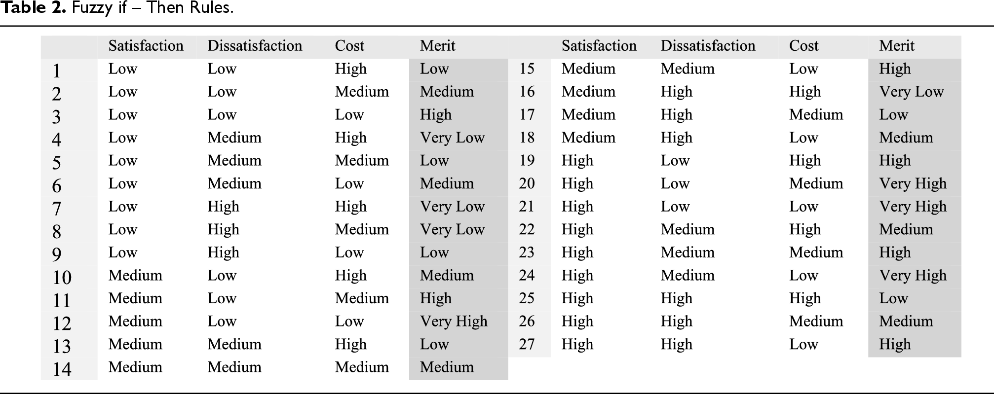
Fuzzy if – Then Rules.
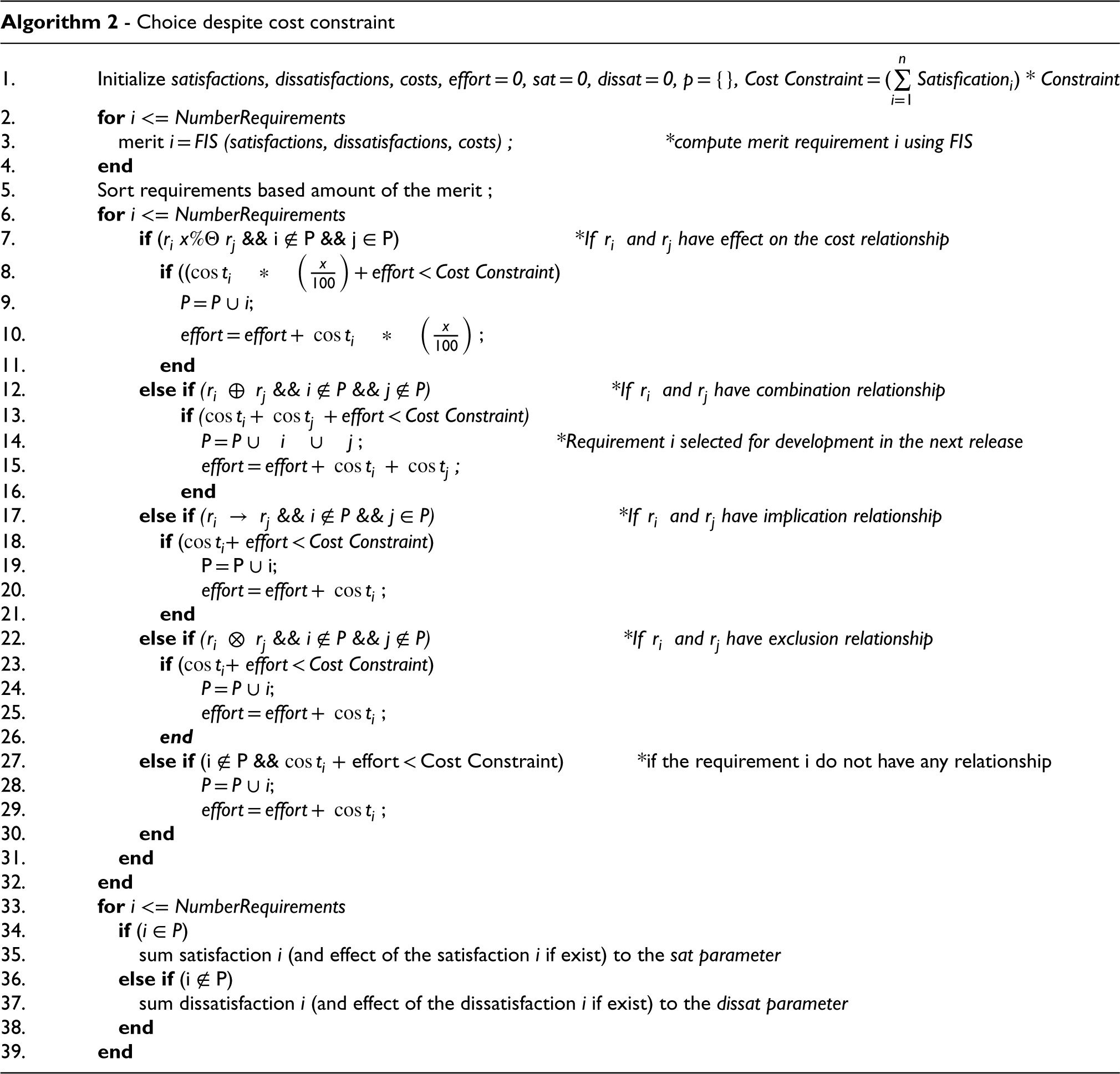
The proposed algorithms can make choices despite cost constraints or dissatisfaction. Depending on the type of restriction, the method of selection is slightly different. Algorithm 2 selects despite the cost constraint, and Algorithm 3 selects despite the dissatisfaction limit. Algorithm 3 determines the exact amount of customer dissatisfaction before product development. In Figure 3, the flowchart of Algorithm 2 is shown.

Flowchart of Algorithm 2.
In this algorithm, the values of cost, satisfaction, dissatisfaction of requirements, as well as the amount of cost constraint are received from the input. Variables are then defined to store the final values. The effort parameter is used to maintain the cost of the selected subset, the sat parameter is used to maintain the satisfaction of the selected requirements, and the dissat parameter is used to maintain the amount of dissatisfaction. The empty set P is used to store selected requirements.
Algorithm 2 first uses the fuzzy inference system to determine the merit of each requirement for development in the next release. It then sorts the requirements based on their merit. In the second step, the algorithm examines the requirements according to their merit. In this step, the relationship between requirements is examined. For example, if the two requirements
Other relations are considered like Algorithm 2. In the third step, the amount of satisfaction and cost of the variables that have been selected and are in the p set are calculated. The final dissatisfaction (FSD) value is also obtained from the difference between TD and dissat. Of course, the FSD value is less than the DS.

One of the main advantages of the two proposed algorithms is their scalability. These algorithms can find the optimal subset of n requirements in time order O(n). In almost all of the previous algorithms presented to solve the NRP problem, the absence of the scalability was a big problem. In linear programming methods, these problems are quite obvious. Also, in metaheuristic algorithms, the quality of the solutions of the algorithms is completely affected when the number of requirements, the number of goals and the limitations increase. In all algorithms proposed to solve the NRP problem, the output solutions are completely affected by the correctness of the input data. This means that if customers’ value assignments to the parameters of the requirements were not accurate, the output solutions would probably not be accurate, and vice versa. Also changing customers’ priorities during project implementation may affect product satisfaction. In the proposed algorithms, increase in flexibility is gained through applying fuzzy data.
Example 3, Materials.
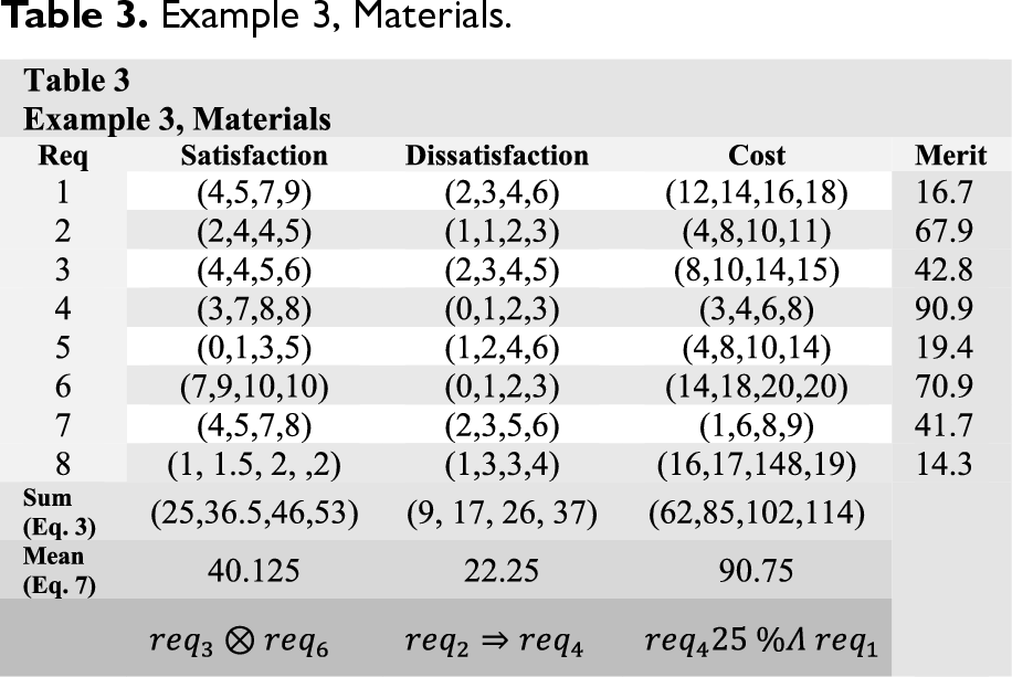
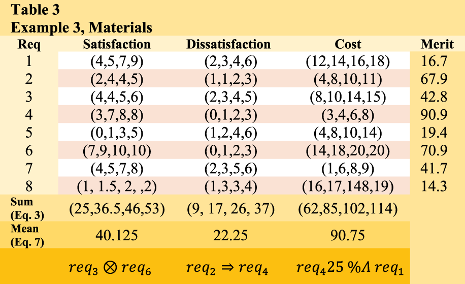
The algorithm first calculates the merit of each requirement, and then commences the selection of requirements for development in the subsequent release, based on the merit order. This process continues until the amount of dissatisfaction parameter exceeds the complement of the dissatisfaction constraint (CDS). Table 4 presents the sequence of requirement selection. In the initial step of the process,
Example 3, Results.
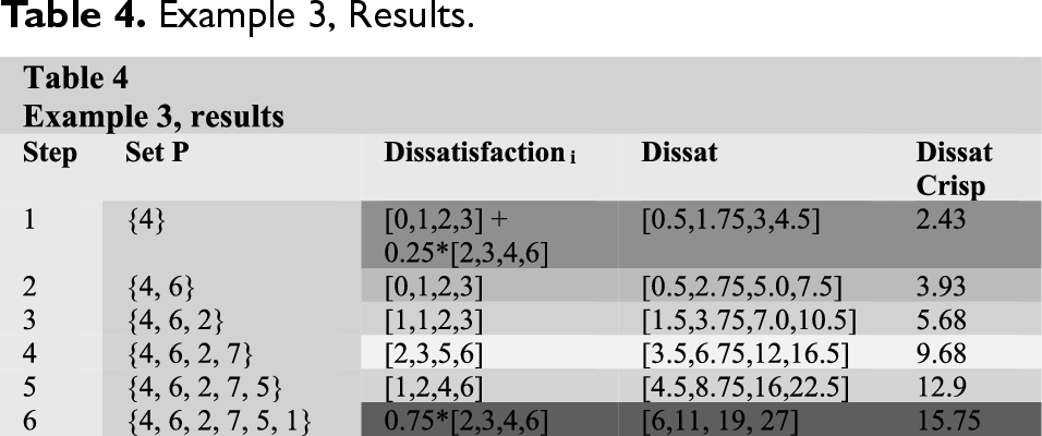

In step 5,
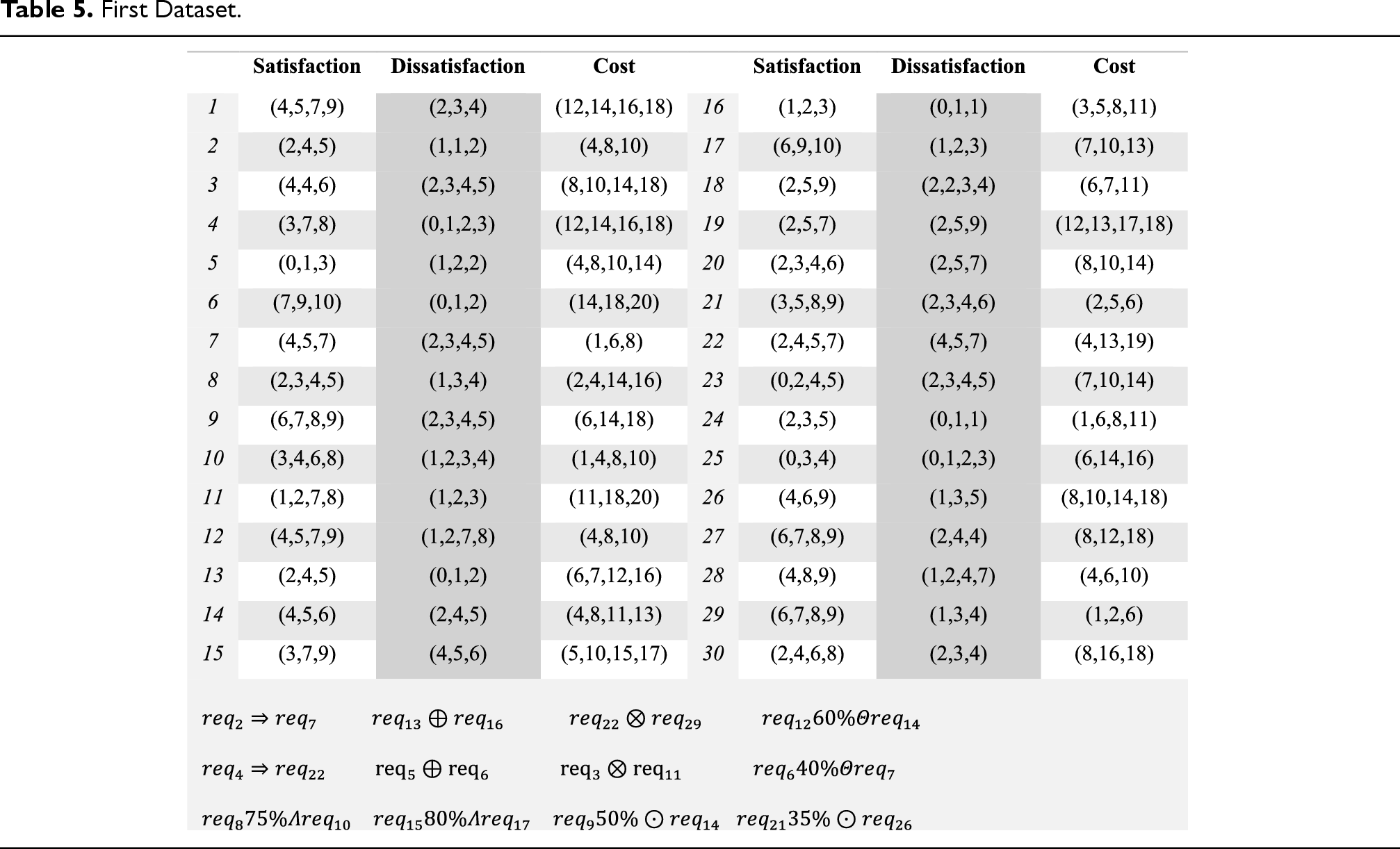
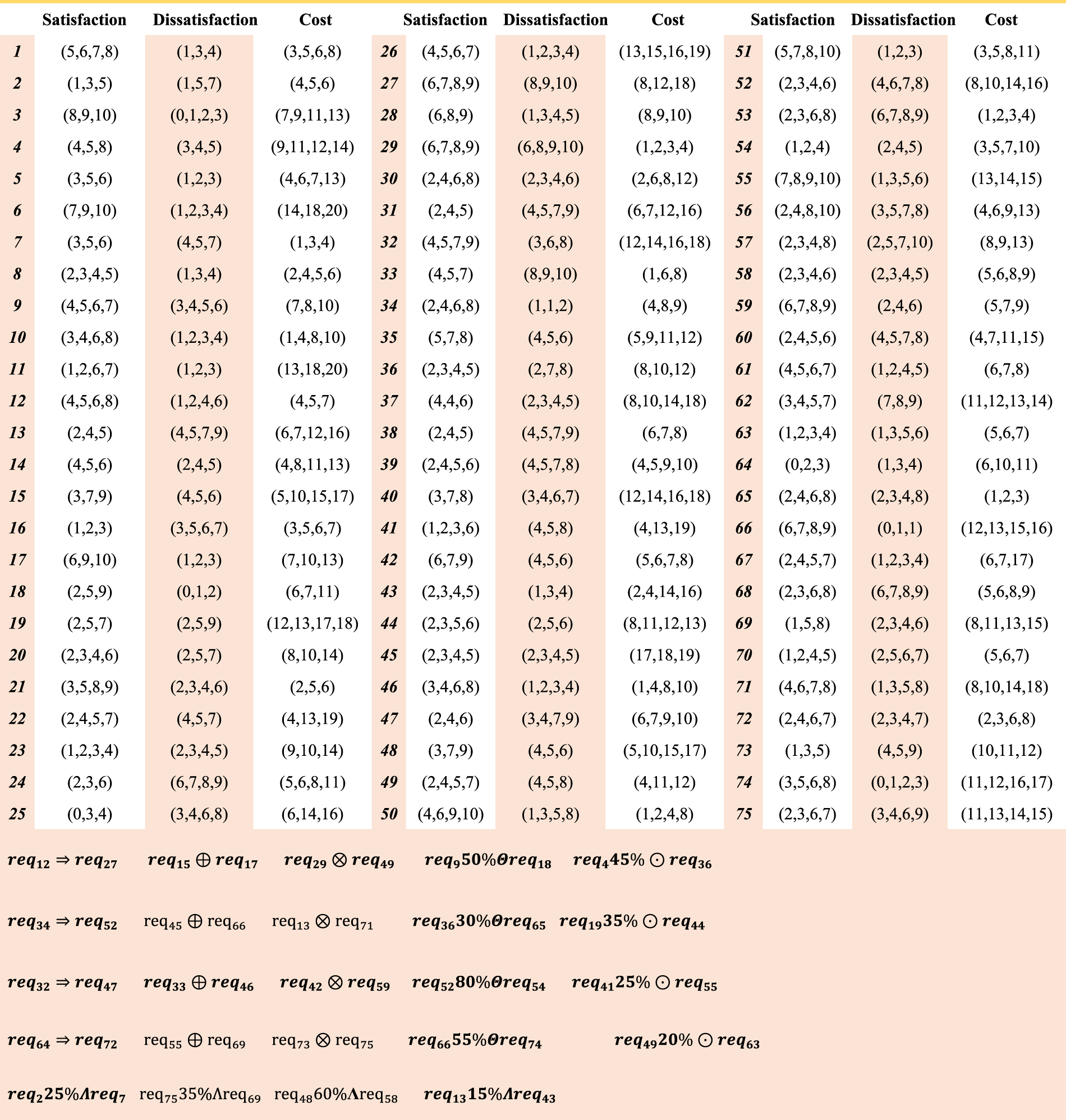
In this section, we will test, evaluate, and compare results. All tests on a PC with CPU core i7-7700HQ 2.80 GHz, RAM 16GB and OS win 10 64bit have been performed by MATLAB software. Since in the previous research, the three goals of satisfaction, dissatisfaction and cost have not been considered at the same time, and there is no dataset with these goals, we have to use dummy data. A small dataset and a large dataset are used for the experiments. Table 5 shows the first dataset. This dataset contains 30 requirements. Customers have been asked about the amount of satisfaction and dissatisfaction for each requirement. The customer assigns a score between 0 and 10 to each requirement. A score of 0 for dissatisfaction of a requirement means not developing this requirement does not create any dissatisfaction for the customer, while score 10 means a lot of dissatisfaction for the customer will arise if the requirement is not developed. For the satisfaction parameter, a score of 0 indicates the lowest level and a score of 10 indicates the highest level of interest for customers. The cost of implementing each requirement is measured by development team experts. Experts also identify relations between requirements. This dataset has 12 constraints of different types of relations. This dataset has 2 relations of type combination, 2 relations of Implication type, 2 relations of Exclusion type, 2 relations of EOC type, 2 relations of EOS type and 2 relations of EOD type. To make more comparisons, the second dataset with 75 requirements and 24 constraints will be used. Table 6 shows the data and constraints of the second dataset. Figure 4 shows the membership functions of the language variables used in the fuzzy inference system. To evaluate the results, the solutions of the proposed algorithms were compared with the FMACRO, IBPSO and Kmeans algorithms. The FMACRO algorithm in the original version was presented as a multi-objective metaheuristic algorithm (two-objective) (Alrezaamiri et al., 2019) and the IBPSO algorithm was presented as a single-objective problem (weighing two goals) (Hamdy & Mohamed, 2019).

Linguistic Variables Membership Functions.
First Dataset.

Second Dataset.

In (del Sagrado and del Águila, 2021) del Sagrado used the combination of the MoSCoW method and clustering algorithms to solve the NRP problem. The results showed that the k-means algorithm is the most suitable clustering algorithm. To find the best number of clusters, the Silhouette method was used. Figure 5 shows the Silhouette values for each number k. The k-means clustering algorithm is simulated with a cluster number of 7 for the first dataset and a cluster number of 8 for the second dataset.

a. Average Silhouette value for first dataset. b. Average Silhouette Value for Second Dataset.
In all tests, the number of iterations of the three algorithms FMACRO, IBPSO and Kmeans was equal to 100, and the number of population members of the algorithms FMACRO and IBPSO was equal to 100. The rest of the parameters of these three algorithms are equal to the values expressed in their articles.
Table 7 shows the results of the run of algorithms on the first dataset with cost constraints (85%, 75% and 65%). The development cost of all requirements is defined as the total cost. An 85% cost constraint means that the selected subset does not have to cost more than 85% of the total cost. These constraints are usually considered by the manufacturing companies due to the reduced cost of the product. The total cost in the first dataset is equal to the trapezoidal number
Algorithm Results with Cost Constraints in the First Dataset.
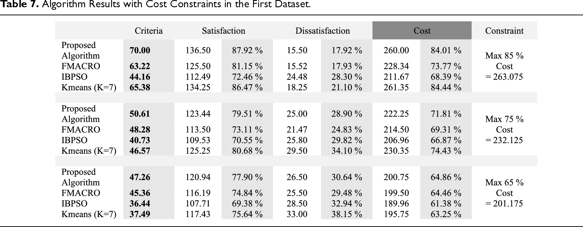

column, we subtract the percentage of dissatisfaction from the percentage of satisfaction in order to obtain an index for easier comparison of algorithms in this test. The higher value shown, the better the performance of the algorithm. Because the FMACRO and IBPSO algorithms are non-deterministic algorithms and the result of each of their runs may be different, the average results of their 10 runs are shown in Table 7 and the following tables. But the proposed algorithms are deterministic algorithms and always get an answer due to greedy choices. Table 7 shows the threshold value constraint on the cost, and all algorithms comply with the allowable cost value. Therefore, to compare the quality of the results, we examine the satisfaction and dissatisfaction values obtained from the algorithms. It has become difficult to compare algorithms due to the existence of three conflicting objectives. We use a criterion to examine. The satisfaction goal is an incremental goal, and in contrast, the dissatisfaction goal is a decreasing goal. That is, the higher the level of satisfaction and the lower the level of dissatisfaction, the better. Therefore, in the criteria.
In the criteria column of Table 7, you can see that the proposed algorithm has obtained a better value in all constraints compared to the other three algorithms. For example, in the 85% constraint, the proposed algorithm was able to select a subset that provided approximately 6.7%, 15.4% and 4.62% more satisfaction than the FMACRO algorithm, the IBPSO algorithm and k-means algorithm, respectively. In addition, the dissatisfaction of the proposed algorithm was approximately equal to the value of the FMACRO algorithm and 10% less than the dissatisfaction of the IBPSO and k-means algorithms. As can be seen in the cost column of Table 7, the FMACRO and IBPSO algorithms were not able to use the maximum allowable limit ceiling as well as the proposed algorithm. For example, in the constraint 85%, the cost of the subset selected by the IBPSO algorithm (211.67) is approximately 17% away from the maximum allowable cost. This is due to weight assignment for the conflicting goals in the IBPSO algorithm. The FMACRO algorithm has been able to reduce this problem to some extent due to the use of non-dominated solutions. By reducing the cost constraint, this problem is greatly reduced in the two algorithms FMACRO and IBPSO, because these algorithms search the middle area of the problem space much more than the marginal areas.
In Figure 6 these points are further explained. The quality of the results of the k-means algorithm was better than that of the IBPSO algorithm, but it was in close competition with the FMACRO algorithm. For example, in the 75% cost constraint, the FMACRO algorithm had a more favourable value, but in the 85% constraint, the k-means algorithm obtained a more appropriate value. The results of the proposed algorithm were of higher quality than the results of the k-means algorithm in all constraints.
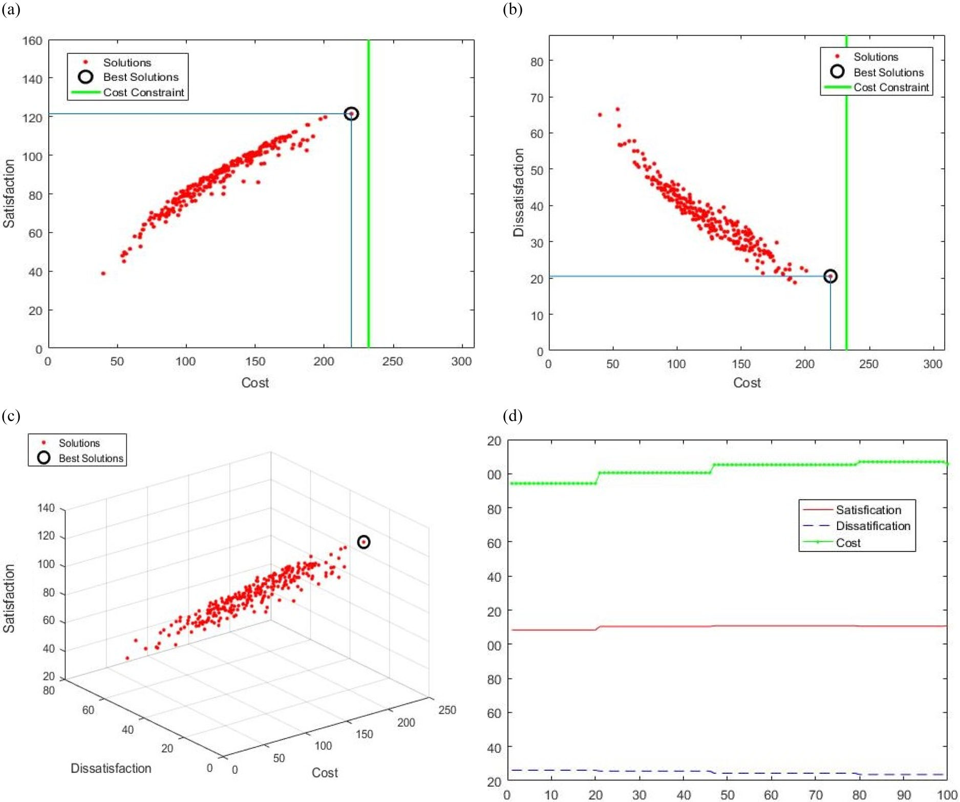
a. Two-dimensional cost-satisfaction figure in the FMACRO algorithm with a cost constraint of 75%. b. Two-Dimensional Cost-Dissatisfaction Figure in the FMACRO Algorithm with a Cost Constraint of 75%. c. Three-dimensional cost-satisfaction-dissatisfaction figure in the FMACRO algorithm with a cost constraint of 75%. d. IBPSO Algorithm Convergence Diagram with Cost Constraint of 75%.
Figure 6 diagrams were obtained by running algorithms in the cost constraint of 75% on the first dataset. These charts are the result of an independent run of two algorithms, FMACRO and IBPSO, and may differ slightly compared to other runs. However, they are useful for describing the results obtained. Figure 6.a and 6.b show a cost constraint of 75% with a crisp value of 232,125 with a green vertical line. The non-dominated solutions discovered are marked as red dots. Among the non-dominated solutions, the best solution is shown with a black circle. Figure 7.a and 7.b identify the requirements selected by the proposed algorithm in green and the unselected requirements in red. The merit value of each requirement determined by the fuzzy inference system is displayed in each cell.
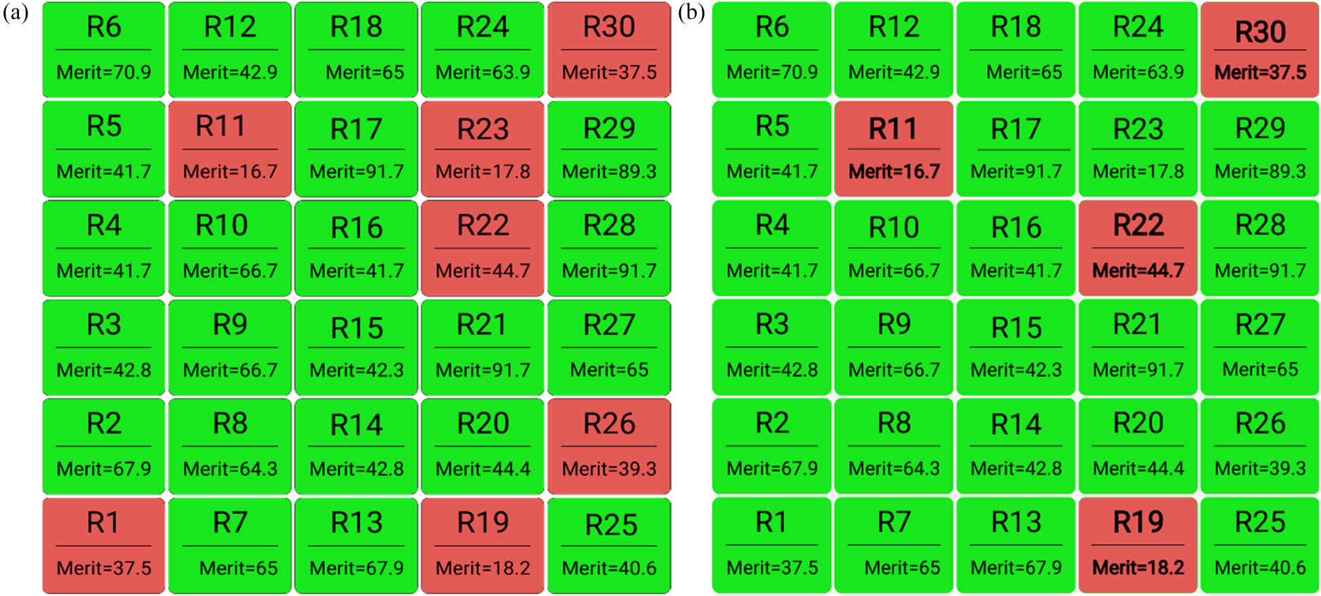
a. Selected and unselected requirements by the proposed algorithm in the cost constraint 75% in first dataset. b. Selected and Unselected Requirements by the Proposed Algorithm in the Cost Constraint 85% in First Dataset.
As it turns out, by changing the cost constraint from 75% to 85%, the three R1, R23, and R26 requirements will be added to the set of selected requirements.
In the next test, we will examine the quality of the results obtained from the algorithms with the restrictions imposed on customer dissatisfaction. This test is performed when the software company wants to be sure of customer dissatisfaction before producing the product. In Table 8, the performances are calculated with 3 constraints of dissatisfaction, so to evaluate the results, we consider the amount of cost and satisfaction obtained from the algorithms as criteria. Once again, we note that customer dissatisfaction means dissatisfaction with the lack of development of requirements that are not selected in the next release.
Constraint Dissatisfaction.

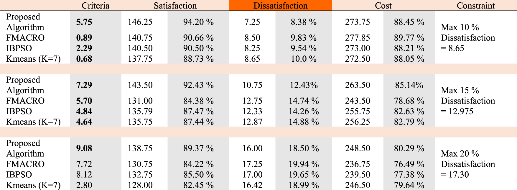
The larger the number of selected requirements, the lower the amount of dissatisfaction; however, the cost increases, which is a negative point. In this experiment, the values of the criteria column are generated by subtracting the percentage of satisfaction from the percentage of cost. According to this criterion, in the 10% dissatisfaction constraint, the proposed algorithm with the 5.75 index performed best. This means that the proposed algorithm is about 4% more satisfied than the other threes algorithms and costs almost the same as the IBPSO and Kmeans algorithm and 1.3% less than the FMACRO algorithm. In the other two constraints, the best results were obtained by the proposed algorithm. According to the Silhouette criterion, the k-means algorithm was run on the first set of data with 7 clusters.
Figure 8.a shows the subset selected by the proposed algorithm with a maximum dissatisfaction constraint of 10%. Due to the exclusion relation between
a. Subset selected by the proposed algorithm with a maximum dissatisfaction constraint of 10%. b. Subset Selected by the Proposed Algorithm with a maximum Dissatisfaction Constraint of 15%. c. subset selected by the IBPSO algorithm with a maximum dissatisfaction constraint of 15%. d. Subset Selected by the FMACRO Algorithm with a maximum Dissatisfaction Constraint of 15%. E. subset selected by the Kmeans algorithm with a maximum dissatisfaction constraint of 15%.
In the following, we will further examine the proposed algorithms by running it on the second dataset. The second dataset has 75 requirements and 24 constraints in which it is impossible to select the optimal subset in the traditional methods. Table 9 shows the results of the algorithms with three cost constraints. In this table, the Criteria column is calculated by subtracting the percentage of satisfaction from the percentage of dissatisfaction. In all three constraints, the proposed algorithm performed much better than the other three algorithms. Especially in the 85% cost constraint, where the subset selected by the proposed algorithm is at least 5.7% less dissatisfied than the other three algorithms and provides much more customer satisfaction.
Results of Algorithms with Three Cost Constraints in the Second Dataset.
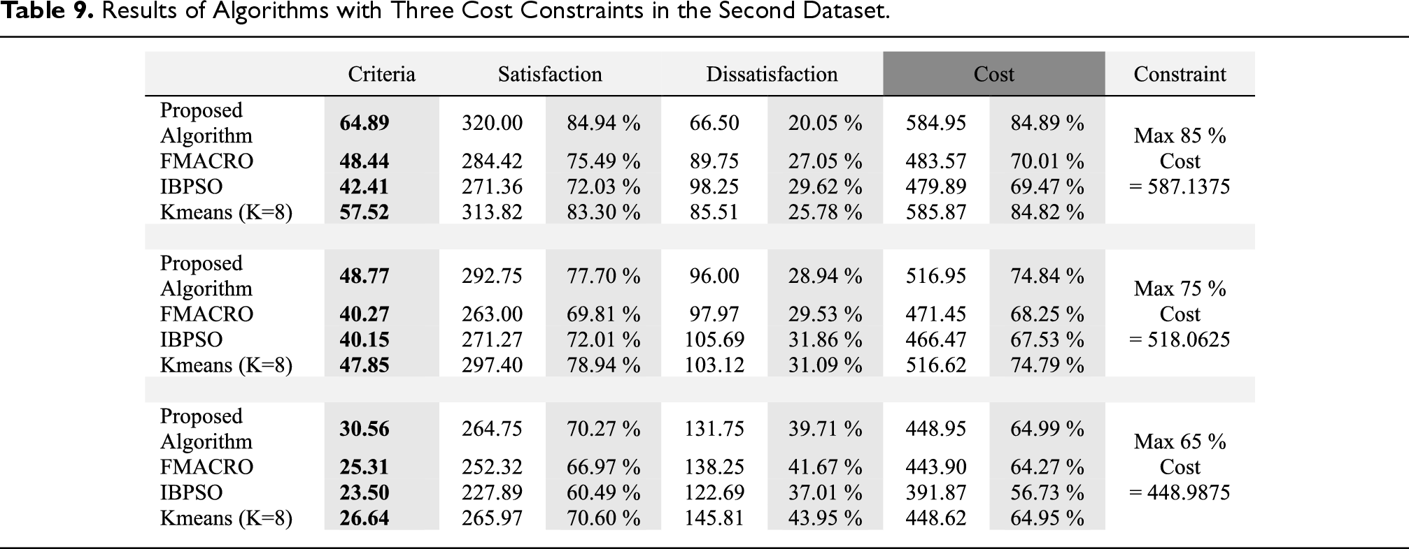
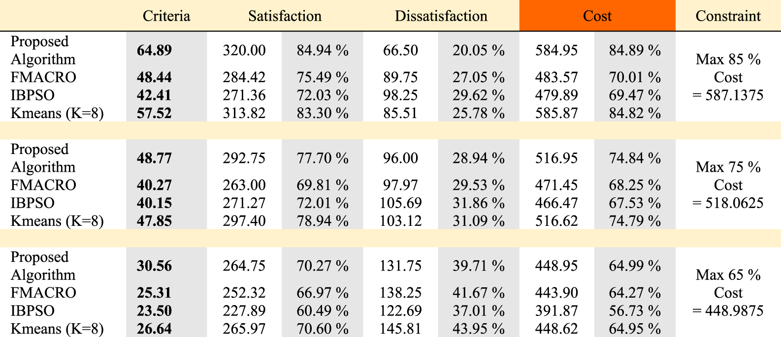
In this test, as well as the test on the first dataset, the proposed algorithm was much better than the FMACRO, IBPSO and Kmeans algorithms; it was able to use the maximum allowable cost ceiling. Selecting more requirements will increase satisfaction and reduce dissatisfaction. Greedy choices have made it possible to use the maximum allowable cost for the proposed method, especially in the high cost constraint. Figures 9.a to 9.c show the value of the best solution selected from the non-dominated solutions discovered by the FMACRO algorithm in the 75% cost constraint. Figure 9.d shows the convergence diagram of the IBPSO algorithm in the 75% cost constraint.
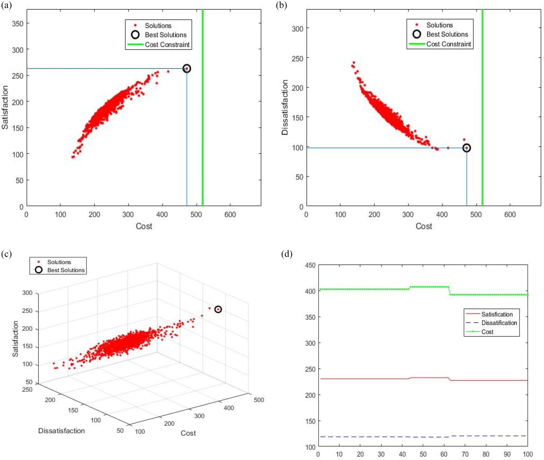
a. Two-Dimensional Cost- Satisfaction Diagram FMACRO Algorithm with a Cost Constraint of 75%. b. Two-dimensional cost- dissatisfaction diagram FMACRO algorithm with a cost constraint of 75%. c. Three-Dimensional Cost-Satisfaction-Dissatisfaction Diagram FMACRO Algorithm with a Cost Constraint of 75%. d. Convergence diagram of IBPSO algorithm with cost constraint of 75%.
In the latest test, we examined the quality of the results obtained from the algorithms, despite three limitations on customer dissatisfaction in the second dataset. Table 10 shows these results. To evaluate the results, we considered the amount of cost and satisfaction of the algorithms. In this experiment, the values of the criteria column are resulted by subtracting the percentage of satisfaction from the percentage of cost. According to this criterion, in the 10% dissatisfaction constraint, the proposed algorithm with the index of 1.94, in the constraint of 15% with the index of 3.96 and in the constraint of 20% with the index of 5.70 performed better than in the other three algorithms.
Results of Algorithms with Three Constraints on Dissatisfaction in the Second Dataset.
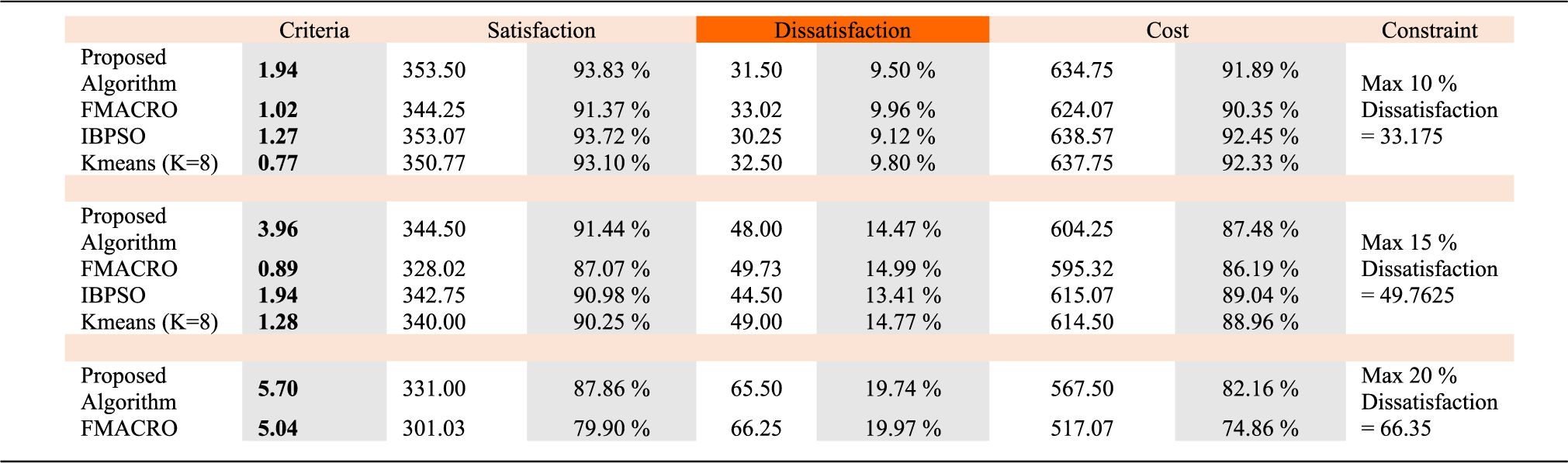
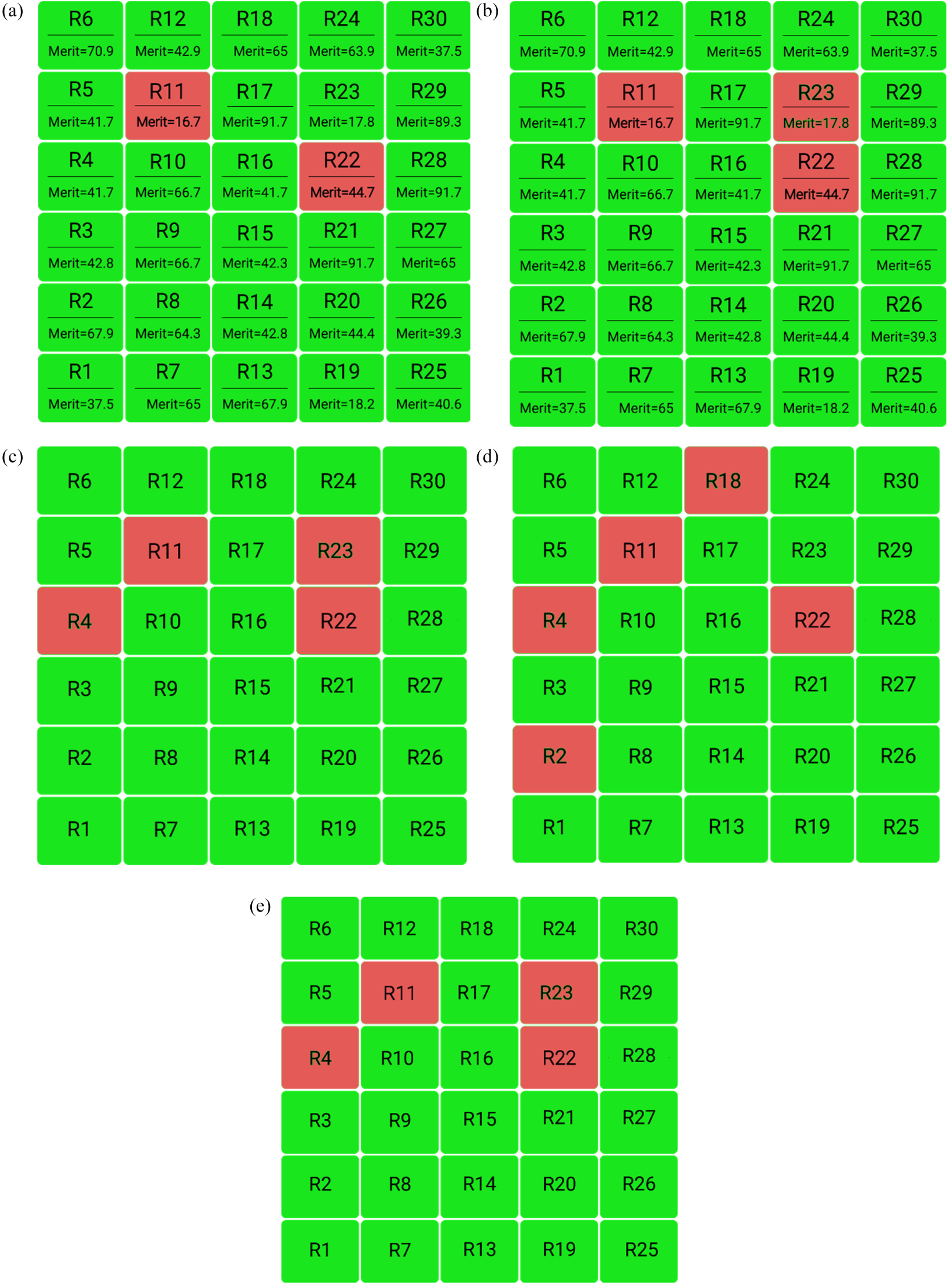
This indicates that the subset selected by the proposed algorithm has always been better than the subset selected by the other three algorithms and has had better results. To better explain the results of this table in Figure 10, the requirements selected by the algorithms are shown schematically. Figure 10.a shows the requirements selected by the proposed algorithm with a 10% dissatisfaction constraint and Figure 10.b with a 15% dissatisfaction constraint. Figures 10.c, 10.d and 10.e show the results of the IBPSO, FMACRO and k-means algorithm selection choices, respectively.
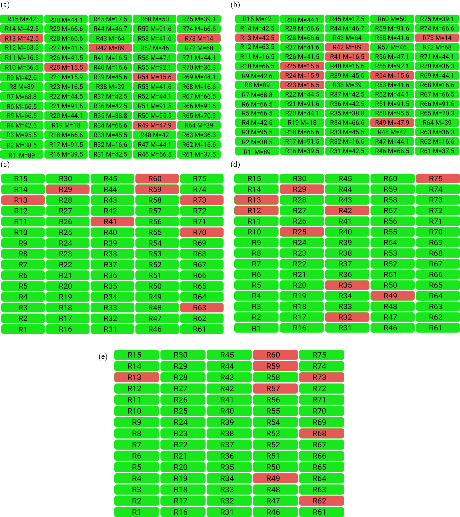
a. Selected set by the Proposed Algorithm with a maximum Dissatisfaction Constraint of 10%. b. Selected set by the proposed algorithm with a maximum dissatisfaction constraint of 15%. Selected set by the IBPSO Algorithm with a maximum Dissatisfaction Constraint of 15%. d. Selected set by the FMACRO algorithm with a maximum dissatisfaction constraint of 15%. e. Selected set by the Kmeans (k = 8) Algorithm with a maximum Dissatisfaction Constraint of 15%.
In Figures 10.a and 10.b, you can see that due to the exclusion constraint between the two
The NRP problem is a challenge in the field of requirement engineering and incremental development methodologies of the software. In this article, we addressed this issue for the first time, with the three goals of cost, satisfaction, and dissatisfaction. In the case of NRP, satisfaction and dissatisfaction goals are not symmetrical. This means that there may be no satisfaction with the development of a requirement, but there may be a great deal of dissatisfaction with its lack of development. It also has several types of threshold value constraints for choices and the inherent relationship between requirements. These three conflicting goals and different constraints make it very difficult for the product manufacturer to choose the optimal subset. To help the development team make intelligent and error-free choices, we've introduced two algorithms. Using the fuzzy inference system, these algorithms determined the merit of the requirements and then made the choices according to the type of threshold value constraint. To make the proposed algorithms more flexible, we converted the input data into fuzzy numbers according to a new method. To make the results more practical, we first introduced and implemented the constraint of the impact on dissatisfaction. For the experiments, the proposed algorithm was compared with the three algorithms FMACRO, IBPSO and Kmeans. In all experiments, the solutions of the proposed algorithms were of higher quality than the other three algorithms. These results show that the choices of the proposed algorithms can provide greater customer satisfaction, reduce dissatisfaction, and lower product prices. One of the most important advantages of the proposed algorithms is their scalability and time complexity of linear order. The next step in this research is to consider other important limitations and goals for software companies. It is also interesting to consider the use of other types of fuzzification and defuzzification on the quality of the results.
Footnotes
Acknowledgements
The authors would like to thank the anonymous reviewers and the associate editor for their insightful comments and suggestions.

Funding
The authors received no financial support for the research, authorship, and/or publication of this article.
Declaration of Conflicting Interests
The authors declared no potential conflicts of interest with respect to the research, authorship, and/or publication of this article.