A fuzzy inference modeling method for nonlinear systems by using triangular pyramid fuzzy system

Abstract

In this paper, a new fuzzy inference modeling method is proposed for nonlinear systems. A proposed triangular pyramid fuzzy system (TPFS) which is proved to have second-order approximation accuracy is employed in the new modeling method. Based on the interpolation mechanism of TPFS, practical systems (which can be described by a group of fuzzy inference rules) can be converted to a simplified linear model with variable coefficients. Expressions of the time-varying local equations appears significantly simple due to the linearity of the model by using the proposed fuzzy modeling method. The approximation performance superiority of the proposed modeling method is demonstrated by simulation results.

Keywords

Fuzzy inference fuzzy systems universal approximation nonlinear systems

1 Introduction

Since it is difficult to analyze a nonlinear system, considerable attention has been drawn to the design and control of complex nonlinear systems. Fuzzy systems have been successfully applied in many areas, e.g., adaptive control [1 –4], theoretical analysis and design of nonlinear systems [5, 6], pattern recognition [7, 8], model approximation [9 –11], etc. Due to its ability to handle linguistics and numerical information, fuzzy modeling technology is of both theoretical and practical importance in various modeling and control applications for complex nonlinear systems.

The universal approximation property of fuzzy systems is a basic problem in its application. As from a mathematical standpoint, a fuzzy system is an approximation function mapping from the input universe to the output universe. Many fuzzy systems have been proved to be able to uniformly approximate any continuous functions defined on compact domains with arbitrary degree of accuracy [12 –18].

A fuzzy modeling method based on the interpolation principle of fuzzy systems [24] is proposed in [19]. In this method, the fuzzy inference mechanism is applied to derive the fuzzy system that describes the controlled plant, such that the model can be transformed into the form of nonlinear differential equations with variable coefficients. However, with the approach proposed in [19], it is rather difficult to analytically investigate the properties (such as stability, controllability and observability) of the nonlinear system. To solve this problem, rectangular membership functions are introduced in [20] to replace conventional triangular membership functions in the fuzzy partition of some universes, so that the variable-coefficient nonlinear model can be converted into a linear model with variable coefficients. However, the approximation property of this fuzzy modeling method is not provided in [20]. Based on the method proposed in [19], fuzzy time is introduced to propose a dynamic fuzzy inference marginal linearization method in [21], and a kind of compensate parameter is applied in the proposed Error-compensated Marginal Linearization Method in [22]. In [23], a proposed fuzzy transformation method is used to construct a fuzzy inference modeling method which is proved to have a first-order approximation accuracy.

It is a challenging problem to improve the approximation property of fuzzy systems. Moreover, for a higher order system, the process of obtaining the coefficients formula of each piecewise model is complicated. Inspired by [20] and to solve these problems, a new linear fuzzy system model TPFS is proposed. The main contributions of this paper include that: 1) it is proved theoretically that the proposed linear fuzzy model TPFS is of second-order approximation accuracy; 2) the proposed method can be applied in fuzzy inference modeling, so that the differential equation of the plant to be controlled can be obtained; and 3) the problem of missing terms in [20] can be solved by using the proposed modeling method. The effectiveness of the proposed modeling method is demonstrated by the comparisons of simulating Van der Pol equation.

2 Preliminaries

In the system under discussion, y (t) and its first-order time derivative $\dot{y} (t)$ are regarded as the input variables, and its second-order time derivative $\ddot{y} (t)$ is regarded as the output variable. Let Y = [a₁, b₁], $\dot{Y} = [a_{2}, b_{2}]$ and $\ddot{Y} = [c, d]$ be the universes of y (t), $\dot{y} (t)$ and $\ddot{y} (t)$ respectively. Denote A = {A_i (y)} _1≤i≤m, $B = {B_{j} (\dot{y})}_{1 \leq j \leq n}$ and $C = {C_{ij} (\ddot{y})}_{1 \leq i \leq m, 1 \leq j \leq n}$ as the fuzzy partitions of Y, $\dot{Y}$ and $\ddot{Y}$ , respectively. Peak points of A_i (y), $B_{j} (\dot{y})$ and $C_{ij} (\ddot{y})$ are denoted by y_i, ${\dot{y}}_{j}$ and ${\ddot{y}}_{ij}$ , respectively.

The form of fuzzy rules can be represented as follows:

$\begin{matrix} If y (t) is A_{i} and \dot{y} (t) is B_{j}, then \ddot{y} (t) is C_{ij} \\ (i = 1, 2, \dots, m; j = 1, 2, \dots, n) . \end{matrix}$ (1)

The fuzzy system using fuzzy rule (1) can be expressed as an interpolation function of two variables as follows: $\ddot{y} (t) = \sum_{i = 1}^{m} \sum_{j = 1}^{n} A_{i} (y (t)) B_{j} (\dot{y} (t)) {\ddot{y}}_{ij},$ (2) where A_i (y (t)) and $B_{j} (\dot{y} (t))$ are usually triangular membership functions.

Theorem 1. [19] The time-invariant fuzzy system generalized by the fuzzy system Equation (2) can be expressed as the following variable coefficients nonlinear differential equation

$\begin{matrix} \ddot{y} (t) & = & S (y (t), \dot{y} (t)) \\ = & a_{1} (y (t), \dot{y} (t)) y (t) + a_{2} (y (t), \dot{y} (t)) \dot{y} (t) \\ + a_{3} (y (t), \dot{y} (t)) y (t) \dot{y} (t) + a_{4} (y (t), \dot{y} (t)), \end{matrix}$ (3)where $a_{1} (y (t), \dot{y} (t)) = \sum_{i = 1}^{m - 1} \sum_{j = 1}^{n - 1} a_{1}^{ij}$ , $a_{2} (y (t), \dot{y} (t)) = \sum_{i = 1}^{m - 1} \sum_{j = 1}^{n - 1} a_{2}^{ij}$ , $a_{3} (y (t), \dot{y} (t)) = \sum_{i = 1}^{m - 1} \sum_{j = 1}^{n - 1} a_{3}^{ij}$ , and $a_{4} (y (t), \dot{y} (t)) = \sum_{i = 1}^{m - 1} \sum_{j = 1}^{n - 1} a_{4}^{ij}$ . Here, $a_{k}^{ij} (k = 1, 2, 3, 4)$ are the coefficients of the local equation. Moreover, if $(y (t), \dot{y} (t)) \notin [y_{i}, y_{i + 1}] \times [{\dot{y}}_{j}, {\dot{y}}_{j + 1}]$ , then $a_{1}^{ij} = a_{2}^{ij} = a_{3}^{ij} = a_{4}^{ij} = 0$ ; if $(y (t), \dot{y} (t)) \in [y_{i}, y_{i + 1}] \times [{\dot{y}}_{j}, {\dot{y}}_{j + 1}]$ , then the coefficients can be calculated by $\begin{matrix} a_{1}^{ij} & = & (- {\dot{y}}_{j + 1} {\ddot{y}}_{ij} + {\dot{y}}_{j + 1} {\ddot{y}}_{i + 1 j} + {\dot{y}}_{j} {\ddot{y}}_{ij + 1} \\ - {\dot{y}}_{j} {\ddot{y}}_{i + 1 j + 1}) / h_{1} h_{2} \end{matrix}$ (4) $\begin{matrix} a_{2}^{ij} & = & (- y_{i + 1} {\ddot{y}}_{ij} + y_{i} {\ddot{y}}_{i + 1 j} + y_{i + 1} {\ddot{y}}_{ij + 1} \\ - y_{i} {\ddot{y}}_{i + 1 j + 1}) / h_{1} h_{2} \end{matrix}$ (5) $a_{3}^{ij} = ({\ddot{y}}_{ij} - {\ddot{y}}_{i + 1 j} - {\ddot{y}}_{ij + 1} + {\ddot{y}}_{i + 1 j + 1}) / h_{1} h_{2}$ (6) $\begin{matrix} a_{4}^{ij} & = & (y_{i + 1} {\dot{y}}_{j + 1} {\ddot{y}}_{ij} - y_{i} {\dot{y}}_{j + 1} {\ddot{y}}_{i + 1 j} - y_{i + 1} {\dot{y}}_{j} {\ddot{y}}_{ij + 1} \\ + y_{i} {\dot{y}}_{j} {\ddot{y}}_{i + 1 j + 1}) / h_{1} h_{2}, \end{matrix}$ (7) where h₁ = y_i+1 - y_i, and $h_{2} = {\dot{y}}_{j + 1} - {\dot{y}}_{j}$ .

The variable coefficient nonlinear ordinary differential equations Equation (3) are called second-order general HX equation.

If $(y (t), \dot{y} (t)) \in [y_{i}, y_{i + 1}] \times [{\dot{y}}_{j}, {\dot{y}}_{j + 1}]$ , the local HX equation can be given by $\ddot{y} (t) = {a_{1}}^{ij} y (t) + {a_{2}}^{ij} \dot{y} (t) + {a_{3}}^{ij} y (t) \dot{y} (t) + {a_{4}}^{ij},$ (8) indicating that the general HX equation is composed by (p - 1) (q - 1) local equations. Consequently, the solution of HX equation can be got, if the local HX equations are piecewisely solved.

3 TPFS

In order to solve the nonlinear problem of the modeling method mentioned in Section 2, a new linear model is proposed. It distinguishes from the general fuzzy system that, in the proposed fuzzy system, triangular meshes and the following form of fuzzy rules are used: $R_{ij} : If (x, y) is P_{ij}, then z is C_{ij},$ (9) where P_ij (i = 1, 2, ⋯ , m ; j = 1, 2, ⋯ , n) are the linguistic terms characterized by the triangular pyramid membership functions and the detailed expression will be given next; C_ij (i = 1, 2, ⋯ , m ; j = 1, 2, ⋯ , n) are the linguistic terms characterized by the triangular membership functions.

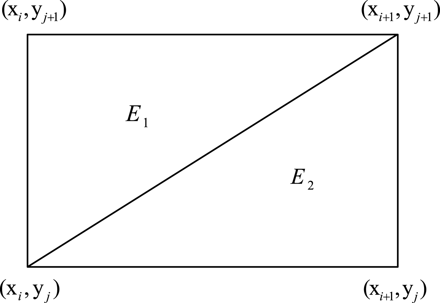
As shown in Fig. 2, a rectangular mesh can be divided into E₁ and E₂. In the domain E₁, the triangular pyramid membership functions with the peak points (x_i, y_i), (x_i+1, y_i+1), (x_i, y_j+1) can be defined by $\begin{matrix} P_{ij} (x, y) & = & \frac{x_{i + 1} y_{j + 1} - x_{i} y_{j + 1}}{m_{1}} \\ - \frac{x_{i + 1} - x_{i}}{m_{1}} y, \end{matrix}$ (10) $P_{i + 1, j + 1} (x, y) = \frac{x_{i} y_{j} - x_{i} y_{j + 1}}{m_{1}} - \frac{y_{j} - y_{j + 1}}{m_{1}} x,$ (11) $\begin{matrix} P_{i, j + 1} (x, y) & = & \frac{x_{i} y_{j + 1} - x_{i + 1} y_{j}}{m_{1}} - \frac{y_{j + 1} - y_{j}}{m_{1}} x \\ - \frac{x_{i} - x_{i + 1}}{m_{1}} y; \end{matrix}$ (12) and in the domain E₂, the triangular pyramid membership functions with the peak points (x_i, y_i), (x_i+1, y_i+1), (x_i+1, y_j) can be defined by $\begin{matrix} P_{ij} (x, y) & = & \frac{x_{i + 1} y_{j} - x_{i + 1} y_{j + 1}}{m_{2}} \\ - \frac{y_{j} - y_{j + 1}}{m_{2}} x, \end{matrix}$ (13) $P_{i + 1, j + 1} (x, y) = \frac{x_{i + 1} y_{j} - x_{i} y_{j}}{m_{2}} - \frac{x_{i + 1} - x_{i}}{m_{2}} y,$ (14) $\begin{matrix} P_{i + 1, j} (x, y) & = & \frac{x_{i} y_{j + 1} - x_{i + 1} y_{j}}{m_{2}} \\ - \frac{y_{j + 1} - y_{j}}{m_{2}} x - \frac{x_{i} - x_{i + 1}}{m_{2}} y . 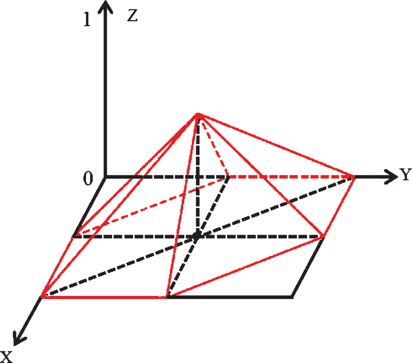\end{matrix}$ (15) where m₁ = x_iy_j - x_i+1y_j + x_i+1y_j+1 - x_iy_j+1 and m₂ = x_i+1y_j - x_iy_j + x_iy_j+1 - x_i+1y_j+1. A simple example of triangular pyramid membership function is illustrated in Fig. 1. A TPFS is similar to a general fuzzy system in that it is also composed by four principal parts, i.e., fuzzifier, fuzzy rule base, fuzzy inference engine and defuzzifier. The expression of a TPFS with singleton fuzzifier, product inference, CRI method, and center of gravity can be represented as follows:

Fig.1

Triangular pyramid membership function.

Fig.2

Division of a rectangular mesh.

In the domain E₁:

$\begin{matrix} S (x, y) \\ = (\frac{x_{i + 1} y_{j + 1} - x_{i} y_{j + 1}}{m_{1}} - \frac{x_{i + 1} - x_{i}}{m_{1}} y) z_{ij} \\ + (\frac{x_{i} y_{j + 1} - x_{i + 1} y_{j}}{m_{1}} - \frac{y_{j + 1} - y_{j}}{m_{1}} x - \frac{x_{i} - x_{i + 1}}{m_{1}} y) z_{i, j + 1} \\ + (\frac{x_{i} y_{j} - x_{i} y_{j + 1}}{m_{1}} - \frac{y_{j} - y_{j + 1}}{m_{1}} x) z_{i + 1, j + 1} . \end{matrix}$ (16)

In the domain E₂:

$\begin{matrix} S (x, y) \\ = (\frac{x_{i + 1} y_{j} - x_{i + 1} y_{j + 1}}{m_{2}} - \frac{y_{j} - y_{j + 1}}{m_{2}} x) z_{ij} \\ + (\frac{x_{i} y_{j + 1} - x_{i + 1} y_{j}}{m_{2}} - \frac{y_{j + 1} - y_{j}}{m_{2}} x - \frac{x_{i} - x_{i + 1}}{m_{2}} y) z_{i + 1, j} \\ + (\frac{x_{i + 1} y_{j} - x_{i} y_{j}}{m_{2}} - \frac{x_{i + 1} - x_{i}}{m_{2}} y) z_{i + 1, j + 1} . \end{matrix}$ (17)

It should be noted that the mesh shape of TPFS is different from that of a general fuzzy system. The triangular mesh has the advantage of solving the problems with a complex domain of definition. This type of mesh has been widely applied in surface reconstruction, reverse engineering, medical imaging, etc. [25]. Another advantage of TPFS is that it uses only one group of membership functions to characterize the fuzzy rule antecedents instead of two groups in a general fuzzy system, such that the fuzzy system can be constructed with significant simplicity; comparatively, two groups of membership functions have to be utilized in general two-input single output fuzzy system.

Furthermore, approximation mechanism and approximation capacities of TPFS are discussed. Obviously, TPFS is a type of piecewise interpolation functions, i.e., in the local region (i, j):

$\begin{matrix} S (x_{i}, y_{j}) & = & f (x_{i}, y_{j}) \\ (i = 1, 2, . . ., m; j & = & 1, 2, . . ., n) . \end{matrix}$ (18)

Theorem 2. Suppose that f ∈ C² (U × V) satisfies f (x_i, y_j) = z_ij (i = 1, 2, . . . , m ; j = 1, 2, . . . , n). For a TPFS S (x, y), it holds that $\begin{matrix} {∥ S - f ∥}_{\infty} & \leq & 3 {∥ \frac{\partial^{2} f}{\partial x^{2}} ∥}_{\infty} {h_{1}}^{2} + 6 {∥ \frac{\partial^{2} f}{\partial x \partial y} ∥}_{\infty} h_{1} h_{2} \\ + 3 {∥ \frac{\partial^{2} f}{\partial y^{2}} ∥}_{\infty} {h_{2}}^{2} . \end{matrix}$

Proof. Take the TPFS in E₂ as an example and define the error as $ɛ (x, y) = S (x, y) - f (x, y) .$

Using first-order Taylor series expansion around an arbitrary point (z, w), the error expands to $\begin{matrix} ɛ (x, y) & = & ɛ (z, w) + \frac{\partial ɛ}{\partial x} |_{(z, w)} (x - z) \\ + \frac{\partial ɛ}{\partial y} |_{(z, w)} (y - w) + r (x, y, z, w), \end{matrix}$ where r (x, y, z, w) is the remainder term defined by

$\begin{matrix} r (x, y, z, w) & = & \frac{\partial^{2} ɛ}{\partial x \partial y} |_{(ξ, η)} (x - z) (y - w) \\ + \frac{1}{2} \frac{\partial^{2} ɛ}{\partial x^{2}} |_{(ξ, η)} (x - z)^{2} \\ + \frac{1}{2} \frac{\partial^{2} ɛ}{\partial y^{2}} |_{(ξ, η)} (y - w)^{2} . \end{matrix}$ (19)

Note that S (x, y) is a linear function of two variables, it follows that

$\begin{matrix} \frac{\partial^{2} ɛ}{\partial x^{2}} |_{(ξ, η)} & = & \frac{\partial^{2} f}{\partial x^{2}} |_{(ξ, η)}, \frac{\partial^{2} ɛ}{\partial y^{2}} |_{(ξ, η)} = \frac{\partial^{2} f}{\partial y^{2}} |_{(ξ, η)}, \\ \frac{\partial^{2} ɛ}{\partial x \partial y} |_{(ξ, η)} = \frac{\partial^{2} f}{\partial x \partial y} |_{(ξ, η)} . \end{matrix}$ (20)

Substituting Equation (20) into Equation (19) yields $\begin{matrix} r (x, y, z, w) & = & \frac{\partial^{2} f}{\partial x \partial y} |_{(ξ, η)} (x - z) (y - w) \\ + \frac{1}{2} \frac{\partial^{2} f}{\partial x^{2}} |_{(ξ, η)} (x - z)^{2} \\ + \frac{1}{2} \frac{\partial^{2} f}{\partial y^{2}} |_{(ξ, η)} (y - w)^{2} . \end{matrix}$

The interpolation property of a TPFS implies that ɛ (x, y) is equal to zero at the points (x_i, y_j), (x_i+1, y_j) and (x_i+1, y_j+1). It then follows that

$\begin{matrix} ɛ (z, w) + \frac{\partial ɛ}{\partial x} |_{(z, w)} (x_{i} - z) + \frac{\partial ɛ}{\partial y} |_{(z, w)} (y_{j} - w) \\ + \frac{1}{2} \frac{\partial^{2} f}{\partial x^{2}} |_{(ξ, η)} (x_{i} - z)^{2} + \frac{1}{2} \frac{\partial^{2} f}{\partial y^{2}} |_{(ξ, η)} (y_{j} - w)^{2} \\ + \frac{\partial^{2} f}{\partial x \partial y} |_{(ξ, η)} (x_{i} - z) (y_{j} - w) = 0, \end{matrix}$ (21) $\begin{matrix} ɛ (z, w) + \frac{\partial ɛ}{\partial x} |_{(z, w)} (x_{i + 1} - z) + \frac{\partial ɛ}{\partial y} |_{(z, w)} (y_{j} - w) \\ + \frac{1}{2} \frac{\partial^{2} f}{\partial x^{2}} |_{(ξ, η)} (x_{i + 1} - z)^{2} + \frac{1}{2} \frac{\partial^{2} f}{\partial y^{2}} |_{(ξ, η)} (y_{j} - w)^{2} \\ + \frac{\partial^{2} f}{\partial x \partial y} |_{(ξ, η)} (x_{i + 1} - z) (y_{j} - w) = 0, \end{matrix}$ (22) $\begin{matrix} ɛ (z, w) + \frac{\partial ɛ}{\partial x} |_{(z, w)} (x_{i + 1} - z) + \frac{\partial ɛ}{\partial y} |_{(z, w)} (y_{j + 1} - w) \\ + \frac{1}{2} \frac{\partial^{2} f}{\partial x^{2}} |_{(ξ, η)} (x_{i + 1} - z)^{2} + \frac{1}{2} \frac{\partial^{2} f}{\partial y^{2}} |_{(ξ, η)} (y_{j + 1} - w)^{2} \\ + \frac{\partial^{2} f}{\partial x \partial y} |_{(ξ, η)} (x_{i + 1} - z) (y_{j + 1} - w) = 0 . \end{matrix}$ (23)

For simplicity, the remainder terms of Equations (21)–(23) are denoted by r₁, r₂, r₃ in the following derivations. Then Equations (21)–(23) can be rewritten as: $\begin{matrix} ɛ (z, w) + \frac{\partial ɛ}{\partial x} |_{(z, w)} (x_{i} - z) \\ + \frac{\partial ɛ}{\partial y} |_{(z, w)} (y_{j} - w) + r_{1} = 0, \end{matrix}$ (24) $\begin{matrix} ɛ (z, w) + \frac{\partial ɛ}{\partial x} |_{(z, w)} (x_{i + 1} - z) \\ + \frac{\partial ɛ}{\partial y} |_{(z, w)} (y_{j} - w) + r_{2} = 0, \end{matrix}$ (25) $\begin{matrix} ɛ (z, w) + \frac{\partial ɛ}{\partial x} |_{(z, w)} (x_{i + 1} - z) \\ + \frac{\partial ɛ}{\partial y} |_{(z, w)} (y_{j + 1} - w) + r_{3} = 0 . \end{matrix}$ (26)

Equations (24)–(26) can be regarded as a linear system with respect to ɛ (z, w), $\frac{\partial ɛ}{\partial x} |_{(z, w)}$ , and $\frac{\partial ɛ}{\partial y} |_{(z, w)}$ . Define the column vectors $ɛ = (ɛ (z, w), \frac{\partial ɛ}{\partial x} |_{(z, w)}, \frac{\partial ɛ}{\partial y} |_{(z, w)})^{T}$ and r = (- r₁, - r₂, - r₃) ^T, and the coefficient matrix $A = [\begin{matrix} 1 & x_{i} - z & y_{j} - w \\ 1 & x_{i + 1} - z & y_{j} - w \\ 1 & x_{i + 1} - z & y_{j + 1} - w \end{matrix}],$

the linear system Equations (24)–(26) can be rewritten in a compact form by $A ɛ = r .$ (27)

Define d and d₁ as follows:

$\begin{matrix} d & = & | A | = h_{1} h_{2}, \\ d_{1} & = & | \begin{matrix} - r_{1} & x_{i} - z & y_{j} - w \\ - r_{2} & x_{i + 1} - z & y_{j} - w \\ - r_{3} & x_{i + 1} - z & y_{j + 1} - w \end{matrix} | \\ = & - r_{1} [(x_{i + 1} - z) (y_{j + 1} - w) - (x_{i + 1} - z) (y_{j} - w)] \\ + r_{2} [(x_{i} - z) (y_{j + 1} - w) - (x_{i + 1} - z) (y_{j} - w)] \\ - r_{3} [(x_{i} - z) (y_{j} - w) - (x_{i + 1} - z) (y_{j} - w)] . \end{matrix}$

According to Cramer’s rule, it holds that ɛ (z, w) = d₁/d. Furthermore, it can be observed that $\begin{matrix} | r_{1} |, | r_{2} |, | r_{3} | \\ \leq \frac{1}{2} {∥ \frac{\partial^{2} f}{\partial x^{2}} ∥}_{\infty} {h_{1}}^{2} + {∥ \frac{\partial^{2} f}{\partial x \partial y} ∥}_{\infty} h_{1} h_{2} + \frac{1}{2} {∥ \frac{\partial^{2} f}{\partial y^{2}} ∥}_{\infty} {h_{2}}^{2}, \end{matrix}$ and

$\begin{matrix} | d_{1} | \\ \leq | - r_{1} [(x_{i + 1} - z) (y_{j + 1} - w) - (x_{i + 1} - z) (y_{j} - w)] | \\ + | r_{2} [(x_{i} - z) (y_{j + 1} - w) - (x_{i + 1} - z) (y_{j} - w)] | \\ + | - r_{3} [(x_{i} - z) (y_{j} - w) - (x_{i + 1} - z) (y_{j} - w)] | \\ \leq 2 h_{1} h_{2} (| r_{1} | + | r_{2} | + | r_{3} |) . \end{matrix}$

It then follows that $\begin{matrix} | ɛ (z, w) | & \leq & 3 {∥ \frac{\partial^{2} f}{\partial x^{2}} ∥}_{\infty} {h_{1}}^{2} + 6 {∥ \frac{\partial^{2} f}{\partial x \partial y} ∥}_{\infty} h_{1} h_{2} \\ + 3 {∥ \frac{\partial^{2} f}{\partial y^{2}} ∥}_{\infty} {h_{2}}^{2} . \end{matrix}$

Since the point (z, w) is arbitrarily selected, it can be finally claimed that $\begin{matrix} {∥ S - f ∥}_{\infty} & \leq & 3 {∥ \frac{\partial^{2} f}{\partial x^{2}} ∥}_{\infty} {h_{1}}^{2} + 6 {∥ \frac{\partial^{2} f}{\partial x \partial y} ∥}_{\infty} h_{1} h_{2} \\ + 3 {∥ \frac{\partial^{2} f}{\partial y^{2}} ∥}_{\infty} {h_{2}}^{2}, \end{matrix}$ which completes the proof.

4 Fuzzy modeling method based on TPFS

It can be observed from Theorem 1 that the expressions of coefficients Equations (4)–(7) are rather complex, and the solution process is consequently complicated. To overcome this problem, a new type of fuzzy modeling method based on a TPFS is introduced in this section. Simpler expressions of coefficients can be obtained due to the linearity of TPFS.

Denote Y = [a₁, b₁], $\dot{Y} = [a_{2}, b_{2}]$ and $\ddot{Y} = [c, d]$ as the universes of y (t), $\dot{y} (t)$ , $\ddot{y} (t)$ , respectively. Let $P = {P_{ij} (y, \dot{y})}_{1 \leq i \leq m, 1 \leq j \leq n}$ and $C = {C_{ij} (\ddot{y})}_{1 \leq i \leq m, 1 \leq j \leq n}$ be the fuzzy partitions of $Y \times \dot{Y}$ and $\ddot{Y}$ . $(y_{i}, {\dot{y}}_{j})$ and ${\ddot{y}}_{ij}$ are the peak points of $P_{ij} (y, \dot{y})$ and $C_{ij} (\ddot{y})$ , respectively. The fuzzy rule base can be defined by $\begin{matrix} R_{ij} : If (y, \dot{y}) is P_{ij}, then \ddot{y} is C_{ij} . \\ (i = 1, 2, \dots, m; j = 1, 2, \dots, n) \end{matrix}$

Theorem 3. The time-invariant fuzzy system generalized by a TPFS can be expressed as the following variable coefficients linear differential equation:

If $(y (t), \dot{y} (t)) \in [y_{i}, y_{i + 1}] \times [{\dot{y}}_{j}, {\dot{y}}_{j + 1}]$ , the (i, j) local equation is given by $\ddot{y} (t) = b_{1}^{ij} \cdot y (t) + b_{2}^{ij} \cdot \dot{y} (t) + b_{3}^{ij} .$

In the domain E₁: ${b_{1}}^{ij} = - \frac{{\dot{y}}_{j + 1} - {\dot{y}}_{j}}{m_{1}} {\ddot{y}}_{i, j + 1} - \frac{{\dot{y}}_{j} - {\dot{y}}_{j + 1}}{m_{1}} {\ddot{y}}_{i + 1, j + 1},$ (28) ${b_{2}}^{ij} = - \frac{y_{i} - y_{i + 1}}{m_{1}} {\ddot{y}}_{i, j + 1} - \frac{y_{i + 1} - y_{i}}{m_{1}} {\ddot{y}}_{ij},$ (29) $\begin{matrix} {b_{3}}^{ij} & = & \frac{y_{i + 1} {\dot{y}}_{j + 1} - y_{i} {\dot{y}}_{j + 1}}{m_{1}} {\ddot{y}}_{ij} \\ + \frac{y_{i} {\dot{y}}_{j + 1} - y_{i + 1} {\dot{y}}_{j}}{m_{1}} {\ddot{y}}_{i, j + 1} \\ + \frac{y_{i} {\dot{y}}_{j} - y_{i} {\dot{y}}_{j + 1}}{m_{1}} {\ddot{y}}_{i + 1, j + 1}; \end{matrix}$ (30)

In the domain E₂: ${b_{1}}^{ij} = - \frac{{\dot{y}}_{j + 1} - {\dot{y}}_{j}}{m_{2}} {\ddot{y}}_{i + 1, j} - \frac{{\dot{y}}_{j} - {\dot{y}}_{j + 1}}{m_{2}} {\ddot{y}}_{ij},$ (31) ${b_{2}}^{ij} = - \frac{y_{i + 1} - y_{i}}{m_{2}} {\ddot{y}}_{i + 1, j + 1} - \frac{y_{i} - y_{i + 1}}{m_{2}} {\ddot{y}}_{i + 1, j},$ (32) $\begin{matrix} {b_{3}}^{ij} & = & \frac{y_{i + 1} {\dot{y}}_{j} - y_{i + 1} {\dot{y}}_{j + 1}}{m_{2}} {\ddot{y}}_{ij} \\ + \frac{y_{i} {\dot{y}}_{j + 1} - y_{i + 1} {\dot{y}}_{j}}{m_{2}} {\ddot{y}}_{i + 1, j} \\ + \frac{y_{i + 1} {\dot{y}}_{j} - y_{i} {\dot{y}}_{j}}{m_{2}} {\ddot{y}}_{i + 1, j + 1} . \end{matrix}$ (33)

Proof. In this proof, only the condition of the domain E₁ is considered, as the expressions of TPFS modeling method in the domain E₂ can be derived in a similar way.

$\begin{matrix} \ddot{y} (t) & = & P_{ij} (y (t), \dot{y} (t))) {\ddot{y}}_{ij} + P_{i, j + 1} (y (t), \dot{y} (t))) {\ddot{y}}_{i, j + 1} \\ + P_{i + 1, j + 1} (y (t), \dot{y} (t))) {\ddot{y}}_{i + 1, j + 1} \\ = & (- \frac{{\dot{y}}_{j + 1} - {\dot{y}}_{j}}{m_{1}} {\ddot{y}}_{i, j + 1} - \frac{{\dot{y}}_{j} - {\dot{y}}_{j + 1}}{m_{1}} {\ddot{y}}_{i + 1, j + 1}) y (t) \\ = & (\frac{y_{i + 1} {\dot{y}}_{j + 1} - y_{i} {\dot{y}}_{j + 1}}{m_{1}} - \frac{y_{i + 1} - y_{i}}{m_{1}} \dot{y} (t)) {\ddot{y}}_{ij} \\ + (\frac{y_{i} {\dot{y}}_{j + 1} - y_{i + 1} {\dot{y}}_{j}}{m_{1}} - \frac{{\dot{y}}_{j + 1} - {\dot{y}}_{j}}{m_{1}} y (t) \\ - \frac{y_{i} - y_{i + 1}}{m_{1}} \dot{y} (t)) {\ddot{y}}_{i, j + 1} \\ + (\frac{y_{i} {\dot{y}}_{j} - y_{i} {\dot{y}}_{j + 1}}{m_{1}} - \frac{{\dot{y}}_{j} - {\dot{y}}_{j + 1}}{m_{1}} y (t)) {\ddot{y}}_{i + 1, j + 1} \\ + (- \frac{y_{i} - y_{i + 1}}{m_{1}} {\ddot{y}}_{i, j + 1} - \frac{y_{i + 1} - y_{i}}{m_{1}} {\ddot{y}}_{ij}) \dot{y} (t) \\ + \frac{y_{i + 1} {\dot{y}}_{j + 1} - y_{i} {\dot{y}}_{j + 1}}{m_{1}} {\ddot{y}}_{ij} + \frac{y_{i} {\dot{y}}_{j + 1} - y_{i + 1} {\dot{y}}_{j}}{m_{1}} {\ddot{y}}_{i, j + 1} \\ + \frac{y_{i} {\dot{y}}_{j} - y_{i} {\dot{y}}_{j + 1}}{m_{1}} {\ddot{y}}_{i + 1, j + 1} . \end{matrix}$ (34)

The local coefficients $b_{k}^{ij} (k = 1, 2, 3)$ on the piece $[y_{i}, y_{i + 1}] \times [{\dot{y}}_{j}, {\dot{y}}_{j + 1}]$ are defined as:

when $(y (t), \dot{y} (t)) \notin [y_{i}, y_{i + 1}] \times [{\dot{y}}_{j}, {\dot{y}}_{j + 1}]$ , $b_{1}^{ij} = b_{2}^{ij} = b_{3}^{ij} = 0,$ when $(y (t), \dot{y} (t)) \in [y_{i}, y_{i + 1}] \times [{\dot{y}}_{j}, {\dot{y}}_{j + 1}]$ , $\begin{matrix} {b_{1}}^{ij} & = & - \frac{{\dot{y}}_{j + 1} - {\dot{y}}_{j}}{m_{1}} {\ddot{y}}_{i, j + 1} - \frac{{\dot{y}}_{j} - {\dot{y}}_{j + 1}}{m_{1}} {\ddot{y}}_{i + 1, j + 1}, \\ {b_{2}}^{ij} & = & - \frac{y_{i} - y_{i + 1}}{m_{1}} {\ddot{y}}_{i, j + 1} - \frac{y_{i + 1} - y_{i}}{m_{1}} {\ddot{y}}_{ij}, \\ {b_{3}}^{ij} & = & \frac{y_{i + 1} {\dot{y}}_{j + 1} - y_{i} {\dot{y}}_{j + 1}}{m_{1}} {\ddot{y}}_{ij} \\ + \frac{y_{i} {\dot{y}}_{j + 1} - y_{i + 1} {\dot{y}}_{j}}{m_{1}} {\ddot{y}}_{i, j + 1} \\ + \frac{y_{i} {\dot{y}}_{j} - y_{i} {\dot{y}}_{j + 1}}{m_{1}} {\ddot{y}}_{i + 1, j + 1} . \end{matrix}$

So Equation (34) can be expressed as the following local equation on one piece $\ddot{y} (t) = b_{1}^{ij} \cdot y (t) + b_{2}^{ij} \cdot \dot{y} (t) + b_{3}^{ij} .$

When $(y (t), \dot{y} (t)) \in Y \times \dot{Y}$ , the general coefficients are defined as $\begin{matrix} b_{1} (y (t), \dot{y} (t)) & = & \sum_{i = 1}^{m - 1} \sum_{j = 1}^{n - 1} b_{1}^{ij}, \\ b_{2} (y (t), \dot{y} (t)) = & \sum_{i = 1}^{m - 1} \sum_{j = 1}^{n - 1} b_{2}^{ij}, \\ b_{3} (y (t), \dot{y} (t)) & = & \sum_{i = 1}^{m - 1} \sum_{j = 1}^{n - 1} b_{3}^{ij}, \end{matrix}$ then, it holds that

$\begin{matrix} \ddot{y} (t) & = & S (y (t), \dot{y} (t)) = \sum_{i = 1}^{m - 1} \sum_{j = 1}^{n - 1} {\ddot{y}}^{ij} (t) \\ = & \sum_{i = 1}^{m - 1} \sum_{j = 1}^{n - 1} [b_{1}^{ij} \cdot y (t) + b_{2}^{ij} \cdot \dot{y} (t) + b_{3}^{ij}] . \\ = & (\sum_{i = 1}^{m - 1} \sum_{j = 1}^{n - 1} b_{1}^{ij}) y (t) + (\sum_{i = 1}^{m - 1} \sum_{j = 1}^{n - 1} b_{2}^{ij}) \dot{y} (t) \\ + \sum_{i = 1}^{m - 1} \sum_{j = 1}^{n - 1} b_{3}^{ij} \\ = & b_{1} (y (t), \dot{y} (t)) y (t) + b_{2} (y (t), \dot{y} (t)) \dot{y} (t) \\ + b_{3} (y (t), \dot{y} (t)), \end{matrix}$ (35) which completes the proof.

The solution of the general differential Equation (35) can be got by solving (m - 1) (n - 1) local equations. Then, the approximating solution of the original model can be got.

It should be noted that Equation (35) is derived from Equations (16), consequently, the estimation of approximation error given by Theorem 2 is valid for Equation (35). It indicates that the differential model based on a TPFS is capable of approximating the original system with second-order approximation accuracy.

5 Simulation studies

In this section, the proposed fuzzy inference modeling method based on a TPFS is compared with two other approaches including: 1) the fuzzy inference modeling method based on Mamdani fuzzy system [19], and 2) the combination model of marginal linearization method [20]. The two methods are generally applied in modeling nonlinear systems. Furthermore, as the second method is a linear method, it is very suitable for comparison with the proposed fuzzy inference modeling method based on a TPFS. The Van der Pol equation is simulated in [19] and [20]. For the sake of convenient comparison, these three modeling methods are used to model the Van der Pol equation with the rule numbers m = 10, n = 10 and m = 12, n = 14, $\ddot{y} (t) - (1 - y^{2} (t)) \dot{y} (t) + y (t) = 0,$ (36) and denoted as Model I, Model II and Model III, respectively. For comparative purposes, the corresponding parameters are assigned the same in different methods.

Let the initial value and simulation time span be $(y (0), \dot{y} (0)) = (2, 0)$ and T = 20, respectively. The detailed simulation steps of the modeling method based on TPFS are listed as follows.

Step 1. Determine the universes Y and $\dot{Y}$ . By using the solutions to Equation (36), we can find the maximum and minimum values of y (t) and $\dot{y} (t)$ which are respectively denoted as y_max, y_min, ${\dot{y}}_{\max}$ and ${\dot{y}}_{\min}$ . For an acceptable range of errors, let the universes be Y = [a₁, b₁] and $\dot{Y} = [a_{2}, b_{2}]$ , where $\begin{matrix} a_{1} & = & y_{min} - 0.1 | y_{min} |, b_{1} = y_{max} + 0.1 | y_{max} |, \\ a_{2} & = & {\dot{y}}_{min} - 0.1 | {\dot{y}}_{min} |, b_{2} = {\dot{y}}_{max} + 0.1 | {\dot{y}}_{max} | . \end{matrix}$

Step 2. Calculate the peak points. Y and $\dot{Y}$ are divided into (p - 1) and (q - 1) parts, respectively. Let $h_{1} = \frac{b_{1} - a_{1}}{p - 1}$ and $h_{2} = \frac{b_{2} - a_{2}}{q - 1}$ . According to Equation (36), it is easy to obtain the peak points as follows: $\begin{matrix} y_{i} & = & a_{1} + (i - 1) h_{1}, i = 1, 2, \cdot \cdot \cdot, m, \\ {\dot{y}}_{j} & = & a_{2} + (j - 1) h_{2}, j = 1, 2, \cdot \cdot \cdot, n, \\ {\ddot{y}}_{ij} & = & (1 - {y_{i}}^{2}) {\dot{y}}_{j} - y_{i}, i = 1, 2, \cdot \cdot \cdot, m, \\ j = 1, 2, \cdot \cdot \cdot, n . \end{matrix}$

Step 3. Calculate the coefficients $b_{k}^{ij} (i = 1, 2, . . ., m, j = 1, 2, . . ., n, k = 1, 2, 3)$ based on Equations (28)–(33).

Step 4. Solve the (m - 1) (n - 1) local equations piecewise with the initial condition y (0) = y₀ and $\dot{y} (0) = {\dot{y}}_{0}$ . let x₁ (t) = y (t), $x_{2} (t) = \dot{y} (t))$ , then the following local state space equations are got. ${\begin{matrix} {\dot{x}}_{1} (t) = x_{2} (t) \\ {\dot{x}}_{2} (t) = b_{1}^{ij} y (t) + b_{2}^{ij} \dot{y} (t) + b_{3}^{ij} . \end{matrix}$

It should be noted that the terminal value of the former piece is used as the initial value of the latter piece when the local state space equations are piecewise solved. It means that these initial values are piecewise generated and transmitted, and the first initial values are y (0) = y₀ and $\dot{y} (0) = {\dot{y}}_{0}$ given in advance.

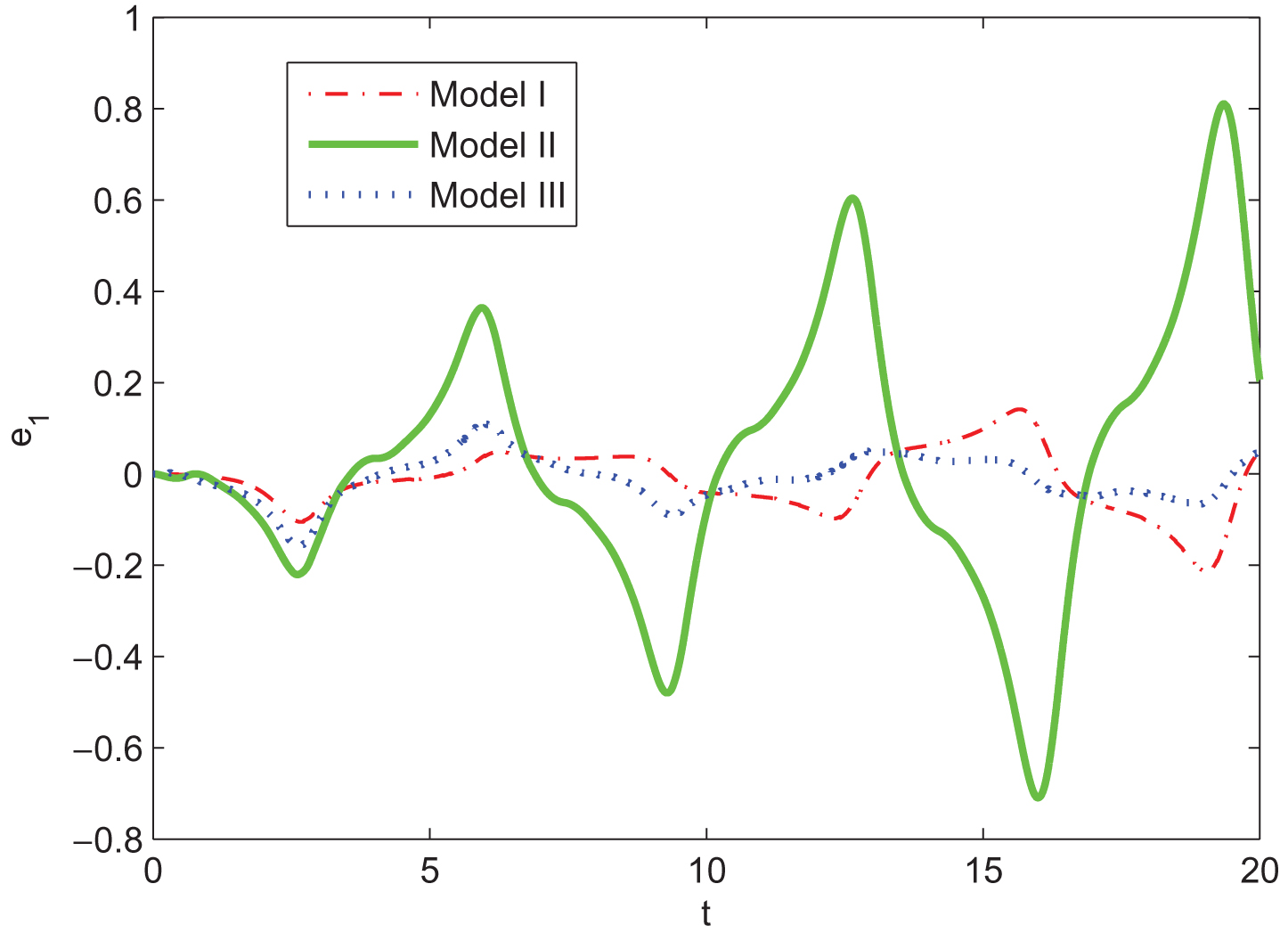
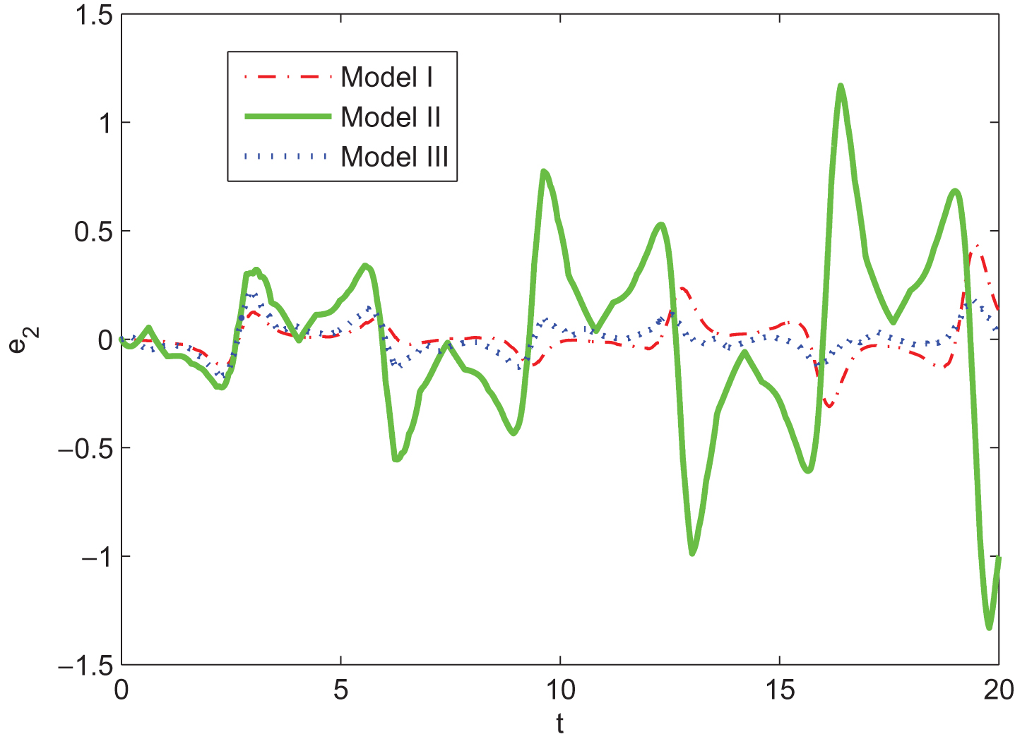
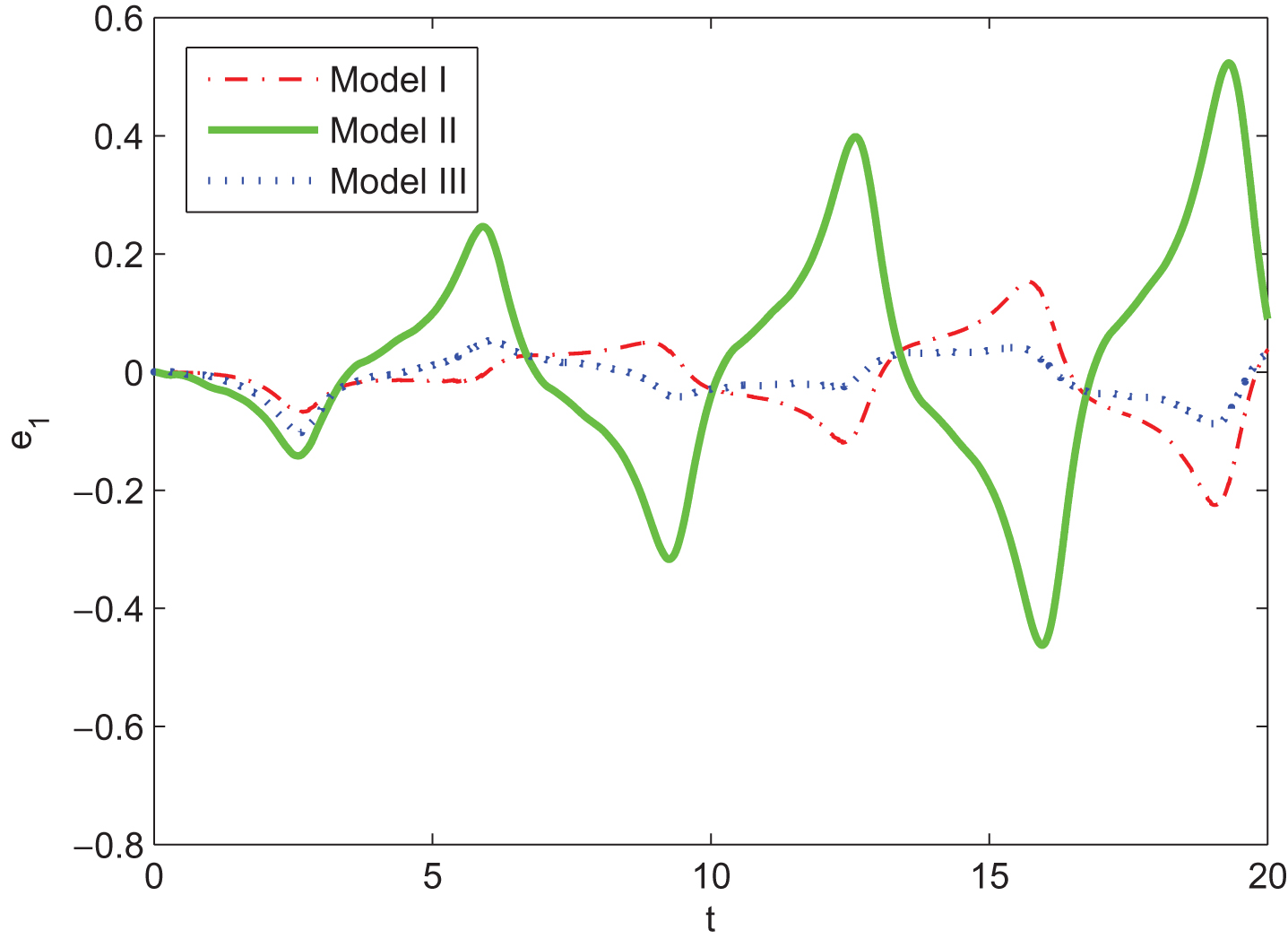
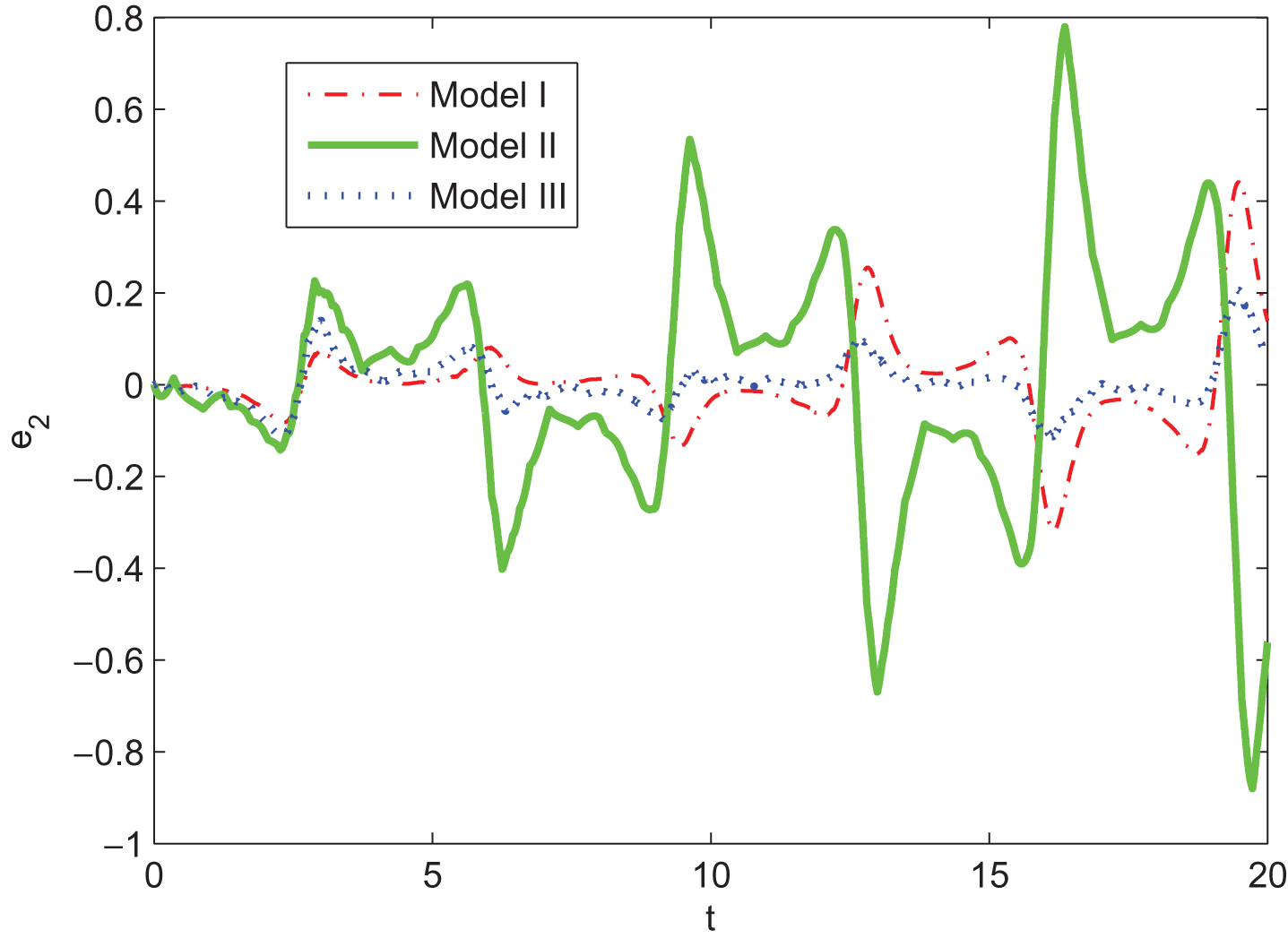
It can be seen from the comparisons of error curves in Figs. 3–6, the approximation error level of Model III is lower than those of Model I and Model II. As listed in Tables 1–4, the maximum and mean errors of Model III are smaller than those of Model I and Model II in each case. In general, the proposed fuzzy modeling method based on TPFS can model Van der Pol equation with superior accuracy over the other two approaches.

Fig.3

Error curves of y of Models I–III (m = 10, n = 10).

Fig.4

Error curves of $\dot{y}$ of Models I–III (m = 10, n = 10).

Fig.5

Error curves of y of Models I–III (m = 12, n = 14).

Fig.6

Error curves of $\dot{y}$ of Models I–III (m = 12, n = 14).

Table 1

Maximum errors of y and $\dot{y}$ of different models (m = 10, n = 10)

Models	Model I	Model II	Model III
Maximum errors of y	0.1418	0.8109	0.1112
Maximum errors of $\dot{y}$	0.4362	1.1690	0.2230

Table 2

Mean errors of y and $\dot{y}$ of different models (m = 10, n = 10)

Models	Model I	Model II	Model III
Mean errors of y	0.0555	0.2225	0.0396
Mean errors of $\dot{y}$	0.0641	0.3089	0.0528

Table 3

Maximum errors of y and $\dot{y}$ of different models (m = 12, n = 14)

Models	Model I	Model II	Model III
Maximum errors of y	0.1527	0.5231	0.0534
Maximum errors of $\dot{y}$	0.4414	0.7801	0.2059

Table 4

Mean errors of y and $\dot{y}$ of different models (m = 12, n = 14)

Models	Model I	Model II	Model III
Mean errors of y	0.0527	0.1489	0.0297
Mean errors of $\dot{y}$	0.5745	0.2046	0.0365

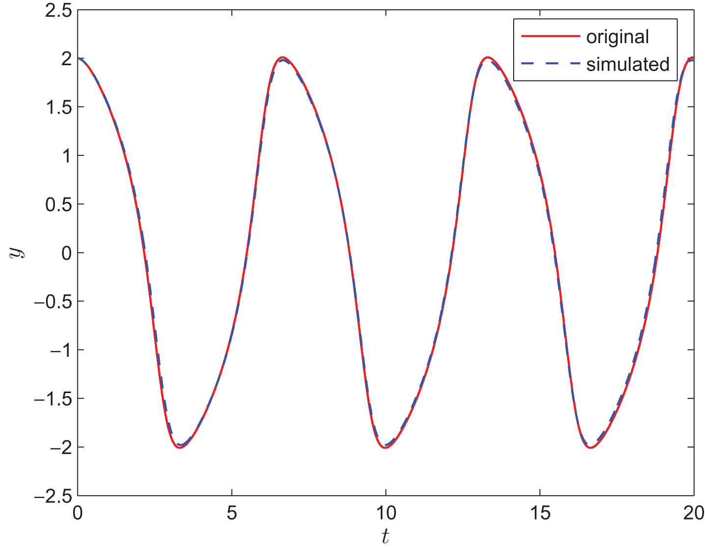
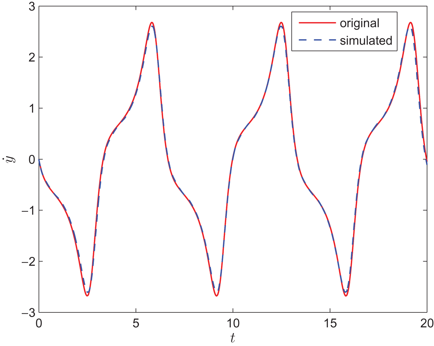
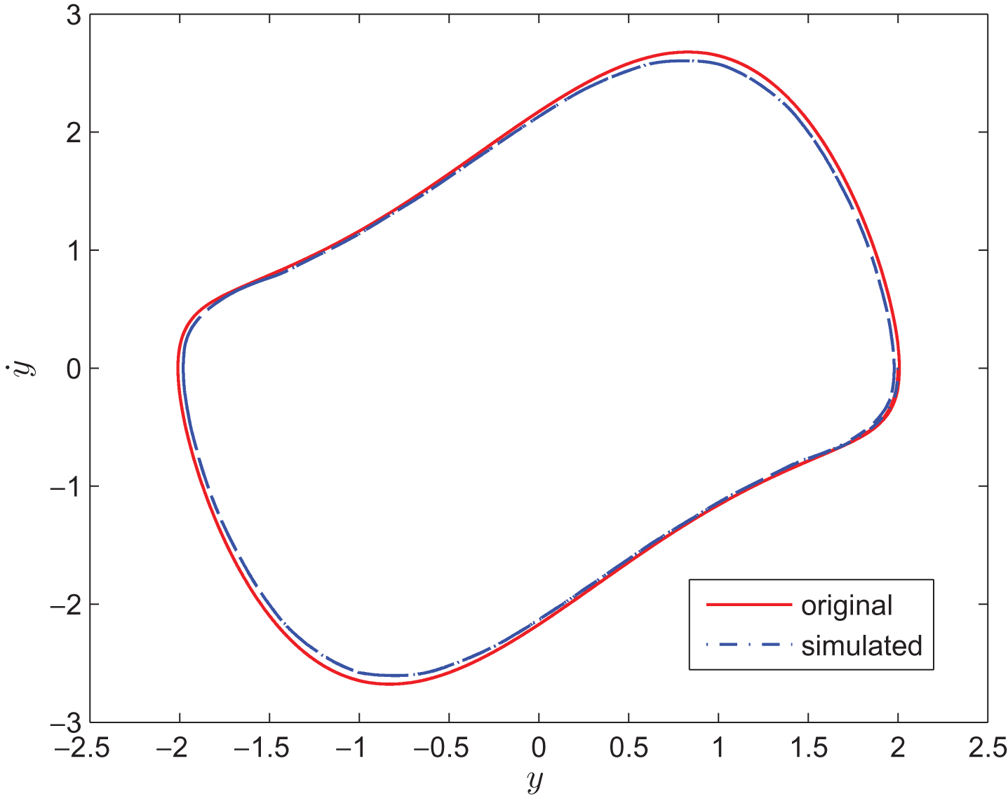
As shown in Figs. 7–9, the approximated curves almost coincide with the original curves, reflecting that the models based on TPFS can approximate the real model with a high accuracy. In other words, the models based on TPFS are very effective.

Fig.7

Approximated and original curves of y (t) of Model III (m = 12, n = 14).

Fig.8

Approximated and original curves of $\dot{y} (t)$ of Model III (m = 12, n = 14).

Fig.9

Approximated and original phase portraits of Model III (m = 12, n = 14).

6 Conclusion

In this paper, a new linear fuzzy modeling method is proposed by using TPFS. With the proposed fuzzy modeling method, a group of data information can be transferred into a fuzzy system represented by a piecewise linear model. It has been proved that second-order approximation accuracy can be achieved by the proposed fuzzy modeling method. The superior approximation performance of the proposed fuzzy modeling method is evaluated by comparative simulation results. Future works on this research will include analysis on the stability of the proposed fuzzy modeling method.

Footnotes

Acknowledgments

The authors would like to thank the Editor-in-Chief, the Associate Editor, and anonymous reviewers for their constructive comments, which helped greatly improve the presentation of this paper. This work was supported by National Science Foundation of China (No. 61473327).

References

Chang

C.Y.

, Hsu

C.H.

, Wang

W.J.

, Chang

C.L.

and Chen

C.Y.

, Operation characteristic control of direct methanol fuel cell liquid feed fuel system using adaptive neuro-fuzzy inference system model, International Journal of Innovative Computing, Information and Control 8(6) (2012), 4177–4187.

Tong

S.C.

and Li

Y.M.

, Fuzzy adaptive robust backstepping stabilization for SISO nonlinear systems with unknown virtual control direction, Information Sciences 18(23) (2010), 4619–4640.

Tong

S.C.

, He

X.L.

and Li

Y.M.

, Direct adaptive fuzzy backstepping robust control for single input and single output uncertain nonlinear systems using small-gain approach, Information Sciences 18(9) (2010), 1738–1758.

Zhang

, Shi

and Xia

, Robust adaptive sliding mode control for fuzzy systems with mismatched uncertainties, IEEE Transactions on Fuzzy Systems 18(4) (2010), 700–711.

Ahmed

A.N.

, El-Shafie

, Karim

O.A.

and El-Shafie

, An augmented wavelet denoising technique with neuro-fuzzy inference system for water quality prediction, International Journal of Innovative Computing, Information and Control 8(10) (2012), 7055–7082.

Gao

H.J.

, Liu

X.M.

and Lam

, Stability analysis and stabilization for discrete-time fuzzy systems with time-varying delay, IEEE Transactions on Systems Man and Cybernetic Part B: Cybernetics 39(2) (2009), 306–317.

Goto

, Yamauchi

, Katafuchi

, Furue

, Sueyoshi

, Uchida

and Hatazaki

, Coal type selection for power plants through fuzzy inference using coal and fly ash property, International Journal of Innovative Computing, Information and Control 7(1) (2011), 29–38.

Wang

, Shi

and Messenger

, Representation of uncertain multichannel digital signal spaces and study of pattern recognition based on metrics and difference values on fuzzy n-cell number spaces, IEEE Trans on Fuzzy Systems 17(2) (2009), 421–439.

Sato

, Miki

and Honda

, A multi-core processor based real-time multi-modal emotion extraction system employing fuzzy inference, International Journal of Innovative Computing, Information and Control 7(8) (2011), 4603–4620.

10.

Wang

G.X.

, Shi

and Wen

C.L.

, Fuzzy approximation relations on fuzzy n-cell number space and their applications in classification, Information Sciences 181(18) (2011), 846–3860.

11.

L.G.

, Su

X.J.

, Shi

and Qiu

J.B.

, Model approximation for discrete-time state-delay systems in the T-S fuzzy framework, IEEE Transaction on Fuzzy Systems 19(2) (2011), 366–378.

12.

Wang

L.X.

, Fuzzy Systems Are Universal Approximators, IEEE International Conference on Fuzzy Systems (1992), pp. 1163–1170.

13.

Wang

L.X.

and Mendel

J.M.

, Fuzzy basis functions, universal approximation, and orthogonal least-squares learning, IEEE T Neural Networks 3(5) (1992), 807–814.

14.

Ying

, Sufficient conditions on general fuzzy systems as function approximators, Automatica 30(3) (1994), 521–525.

15.

Ying

and Chen

, Necessary conditions for some typical fuzzy systems as universal approximators, Automatica 33(7) (1997), 1333–1338.

16.

Ying

, General SISO Takagi-Sugeno fuzzy systems with linear rule consequent are universal approximators, IEEE Transactions on Fuzzy Systems 6(4) (1998), 582–587.

17.

Ying

, Sufficient conditions on uniform approximation of multivariate functions by general Takagi-Sugeno fuzzy systems with linear rule consequent, IEEE Transactions on Systems, Man, and Cybernetics - Part A: Systems and Humans 28(4) (1998), 515–520.

18.

Ying

, Ding

, Li

and Shao

, Comparison of necessary conditions for typical Takagi-Sugeno and Mamdani fuzzy systems as universal approximators, IEEE Transactions on Systems, Man, and Cybernetics - Part A: Systems and Humans 29(5) (1999), 508–514.

19.

H.X.

, Wang

J.Y.

and Miao

Z.H.

, Modelling on fuzzy control systems, Science in China Series A: Mathematics 45(12) (2002), 1506–1517.

20.

H.X.

, Wang

J.Y.

and Miao

Z.H.

, Marginal linearization method in modeling on fuzzy control systems, Progress in Nature Science 13(7) (2003), 489–496.

21.

Wang

D.G.

, Song

W.Y.

and Shi

, Approximation to a class of non-autonomous systems by dynamic fuzzy inference marginal linearization method, Information Sciences 245 (2013), 197–217.

22.

Wang

D.G.

, Chen

C.L.

and Song

W.Y.

, Error-compensated marginal linearization method for modeling a fuzzy system, IEEE Transactions on Fuzzy Systems 23(1) (2015), 215–222.

23.

Yuan

X.H.

, Li

H.X.

and Yang

, Fuzzy system and fuzzy inference modeling method based on fuzzy transformation, Acta Electronica Sinica 41(4) (2013), 674–680.

24.

H.X.

, Interpolation mechanism of fuzzy control, Science in China Series E: Technological Sciences 28(3) (1998), 259–267.

25.

J.Y.

and Lee

, The advantages of triangular and tetrahedral edge elements for electromagnetic modeling with the finiteelement method, IEEE Transactions on Antennas and Propagation 45(9) (1997), 1431–1437.