
Abstract
Maintaining human physical and mental health depends on sleep; insufficient sleep results in illness. Many deep learning (DL) and machine learning (ML) based sleep stage classification (SSC) algorithms have been proposed in the last ten years. However, insufficient feature uniqueness, intricate deep learning architectures, a great deal of hyperparameter adjustment, and low accuracy in classifying sleep stages make SSC difficult. This paper presents SSC based on spectral, texture, and temporal features of electroencephalogram (EEG) features and a lightweight Deep Convolution Neural Network (DCNN) and Long Short-Term Memory (LSTM). The DCNN helps to improve the correlation and connectivity features of EEG, and the LSTM helps to boost the temporal depiction and long-term connectivity of EEG features. It uses Wavelet Packet Transform (WPT) based soft thresholding to minimize noise and artifacts in the EEG signal. The improved Spider Monkey Optimization (ISMO) algorithm selects the decisive features from the multiple EEG features. The suggested WPT-ISMO-DCNN-LSTM-based SSC scheme's effectiveness is estimated on the sleep-European Data Format (Sleep-EDF) dataset based on accuracy, recall, precision, F1-score, trainable parameters, and recognition time. The WPT-ISMO-DCNN-LSTM-based SSC scheme provides an accuracy of 99%, precision of 1, Kohen's Kappa rate of 0.9878, 0.9921, recall of 0.99, and F1-score of 0.99, outperforming the existing state of the art. The WPT-ISMO-DCNN-LSTM provides an accuracy of 99% for 2-class SSC, 99.70% for 3-class SSC, 98.50% for 4-class SSC, 99.30% for 5-class SSC, and 99% for 6-class SSC for 350 features. The proposed algorithm offers 5.9 M trainable parameters and a total training time of 498 s for a 6-class SSC.
Keywords
Introduction
Sleep is a crucial part of our daily life. We sleep for about one-third of our lives. Proper sleep reduces fatigue and enhances our brain's and other organs’ functioning (Lambert & Peter-Derex, 2023; Raghupathy et al., 2024). The fast-paced lifestyle has increased stress in daily life, resulting in poor sleep quality. Inadequate sleep and irregularities in the sleep are significant causes of sleep-related diseases such as depression, hypertension, and the requirement for angiocardiology. As a result, getting enough quality sleep is critical for living a healthy life (Chen et al., 2023; Fu et al., 2023). Sleep stage analysis is the first step in detecting a sleep disturbance and may be done utilizing polysomnographic (PSG) data collected during sleep hours (Phyo et al., 2023).
PSG signal data includes EEG, electromyography (EMG), Electrooculography (EOG), electrocardiography (ECG), and other biological signals. EEG is a noninvasive technique for recording cerebral cortex activity signals. The five frequency divisions that categorize EEG signals are the alpha, beta, theta, delta, and gamma bands. Neurological or sleep abnormalities can be identified and monitored using the amplitude and frequency of the EEG signal (Abdollahpour et al., 2022; Goshtasbi et al., 2022).
The American Academy of Sleep Medicine's (AASM's) recommendations divide the five phases of sleep into waking stages 1–4 (N1, N2, N3, N4) and rapid eye movement (REM). Electrical activities recorded by sensors on various body areas distinguish between these sleep phases. The alpha or higher frequency band reflects high EMG values and frequent eye movements during the wake period. The occupancy of the alpha during more than 50% of the period, theta activity, vertex waves, and slow rolling eye movement are all indicators of sleep stage N1. Sleep spindles recorded fewer than 180 s apart indicate stage N2 (Park et al., 2023).
Delta activity represents the N3 stage of sleep. The lowest EMG signals and the appearance of sawtooth waves during REM can be used to identify the N3 sleep state. Clinical professionals manually analyze the EEG signals for sleep stage analysis (Loh et al., 2020). Because of boredom, exhaustion, and the expert's limited expertise, manually grading the different stages of sleep is a challenging and time-consuming operation that is prone to mistakes. A human expert would find it challenging to analyze the signal due to the rapid variations between different sleep phases. Researchers have proposed an automatic SSC that uses artificial intelligence (AI) to overcome the limitations of manual SSC systems (Satapathy & Loganathan, 2021).
Various ML and DL schemes have been presented for the SSC. Accurate and automated SSC is essential for diagnosing sleep disorders and understanding sleep patterns (Sekkal et al., 2022). Traditional manual scoring by sleep experts is time-consuming, subjective, and prone to inconsistencies. Existing ML and DL models have improved classification accuracy but often suffer from high computational complexity and redundant features, leading to inefficiencies in real-time applications (Cui et al., 2018; Tsinalis et al., 2016; Wang & Wu, 2018a). Feature selection enhances model performance by reducing dimensionality while preserving discriminative information. However, conventional optimization techniques struggle to balance exploration and exploitation effectively. This paper proposes a DCNN-based SSC with efficient feature selection to enhance SSC performance using EEG signals from the Sleep-EDF dataset. The proposed approach aims to improve classification accuracy, reduce computational burden, and provide a robust framework for real-time sleep analysis.”
This paper presents the sleep stage classification using multiple EEG features and DCNN. The significant contributions of the article are summarized as –
Extraction of multiple EEG features such as time domain features, spectral domain features, and statistical features to improve the EEG signal representation. EEG signal enhancement using wavelet packet transform-based soft thresholding to minimize the noise and artifacts in EEG Selection of decisive features from multiple EEG features using improved SMO based on competitive learning strategy to improve the search space, convergence and solution diversity of traditional SMO. Implement a lightweight DCNN to improve the feature representation for sleep stage classification. The effectiveness of the suggested SSC scheme is estimated on the Sleep-EDF dataset using accuracy, recall, precision, F1-score, total trainable parameters, and recognition time of the scheme.
The remaining article is arranged as follows: Section II reviews recent work for SSC. Section III elaborates on the WPT-ISMO-DCNN-LSTM-based SSC scheme in detail. Section IV gives the simulation results and discusses the suggested SSC scheme. Lastly, section V depicts the conclusion and provides the future scope for the conceivable upgrading of the current work.
Numerous works have been presented for ML and DL-based SSC in the last decade. The DL-based SSC techniques have shown significant enhancement over the performance of ML-based SSC techniques. The DL-based schemes have shown superior feature representation capability of the EEG signal and improved the distinctiveness of the features.
Tsinalis et al. (2016) presented the SSC's sparse stack auto-encoder (SSAE) using wavelet transform features. Using 20 EEG signal recordings from the sleep-EDF database, they could classify the five sleep stages with 78% accuracy using their proposed approach. Cui et al. (2018) examined CNN and a fine-grained segment for sleep stage analysis using multichannel EEG. Six EEG signals, two EOG channels, and three EMG channels were among the eleven data channels they provided to CNN, each lasting 30 s. Their recommended method had an accuracy of 92.20% on average. Next, using single-channel EEG data, Wang and Wu, (2018a) published a compact CNN for sleep stage analysis. They injected the power spectral density of an unprocessed EEG sample into a deep architecture. It has been shown that long short-term memory gathers more temporal data than the standard CNN architecture (Xu et al., 2020). Conventional methods need human scoring and are computationally expensive. Ozal Yildirim et al. (2019) developed a one-dimensional CNN for the SSC based on electrooculogram (EOG) and EEG inputs to overcome this problem. To address the class imbalance brought on by a higher proportion of standard samples and a lower proportion of ill samples, they used unique mean square false error and mean false error (Mousavi et al., 2019). DL-based sleep stage scoring usually led to over-fitting and increased resource consumption because of the low quality of the raw data. Blanco et al. (2020) proposed a separable CNN for sleep stage detection using an EEG signal that produced an accuracy of 85.22% to provide robustness to the challenges mentioned above. To learn the diverse and rich feature representation of the EEG signal, Zhang et al. (2020) presented orthogonal CNN (OCNN), which accepts the time-frequency domain data obtained by the Hilbert-Huang transform (HHT). DCNN for the child SSC, which restores the hidden layer properties to the input layer, was also studied by Huang et al. (2020). For Sleep Dataset of Child Patients (SDCP), it obtained an accuracy of 84.27%, while for the sleep-EDFx database, it obtained a 90.89% accuracy. It was shown that CNN performance may be improved by adding a spectral-temporal representation of the signal over the raw signal (Kim et al., 2020). K-complexes are essential for sleep analysis to characterize complex sleep patterns (Al-Salman et al., 2024). Salman et al. (2022) suggested the segment-level features and SVM for the SSC. It resulted in 96.3%, 93.2%, and 95.4% specificity, sensitivity, and accuracy for the SSC. Further, Salman et al. divided the EEG signal into small segments, and every segment is decomposed into 5 levels using the discrete wavelet transform. The coefficients are clustered using the K-means clustering algorithm. The least square SVM provides an overall accuracy of 97.4% for the six-stage SSC. However, the performance of ML-based techniques is limited for larger datasets and provides poor feature depiction.
Ji et al. (2024) suggested MixSleepNet, which combines the graph convolutional network and 3-D convolution, to improve the feature depiction of multi-channel EEG for the SSC. It provided 83% and 81.2% accuracy for the SSC for ISRUC-S3 and ISRUC-S1 datasets, respectively. However, the complexity and total learnable parameters are higher (2.4 M). Pei et al. (2024) provided the mel-frequency cepstral coefficients (MFCC), which have shown impressive results for speech recognition for the SSC based on EEG. However, the MFCC-based SSC suffers from low-frequency resolution and spectral leakage problems. Kayabekir and Yağanoğlu (2024) suggested SPINDILOMETER, which consists of bi-spectrum score features, wavelet features, non-Gaussianity score features, and power density features for EEG representation (k-complex and sleep spindles). It offered 94.67% accuracy for single-channel EEGs of 72 subjects. Wang et al. (2024a) suggested CareSleepNet, which encompasses the convolution transformer and encoder based on the cross-modality between EOG and EEG for providing superior connectivity in global and local attributes of the EEG features. It is observed that the connectivity between EOG and EEG enhances the SSC results. However, the system's effectiveness is limited because of extensive parameter tuning. Using explainable ML models, Hamouda et al. (2024) investigated how multi-channel EEG helps enhance SSC results. It offered an overall accuracy of 87.9% for SSC for the sleep-EDF dataset. It provided better interpretability and explainability of the SSC system to enhance trust in the SSC system. Wang et al. (2024b) explored multiple CNN to enhance the time-invariant features of the EEG, ECG, EOG, and EMG. It provides a superior correlation between global and local attributes of the PSGs. Zhang et al. (2024) presented a multimodal SSC based on EEG and EOG based on the 2-stream encoder-decoder framework. It used an attention scheme for multiscale fusion and creating saliency in features. The transformer module has been employed to depict long-term temporal features, providing 85.2% and 88.9% accuracy for the SleepEDF-153 and Sleep-EDF-39 datasets. Satapathy et al. (2024) suggested a multimodal SSC based on EOG, EEG, and EMG, based on frequency-domain, entropy-based, time-domain, statistical, and non-linear features. It utilized the RelieF feature selection algorithm to choose salient features. It offered 91.55% accuracy for the ensemble AdaBoost-RF classifier for 6-class SSC. However, it fails to provide promising results for multi-class SSC.
Thus, the following gaps are identified from the comprehensive survey of various SSC techniques.
It is observed that the outcomes of the DL framework are highly affected by the type and distinctiveness of the EEG features (Cui et al., 2018; Dhake & Angal, 2022; Hassan et al., 2015). Most DL frameworks have complex network architecture, more significant trainable parameters, and extensive hyperparameter tuning (Yildirim et al., 2019). Poor feature representation due to redundant and non-salient features. Performs poorly for complex sleep patterns because of the inability to capture local variations in the temporal domain. Less robust against the noise and artifacts, and the Low-frequency resolution problem, which provides poor results for low-frequency EEG signals (Al-Salman et al., 2023). Poor focus on the textural pattern of the EEG signal for sleep analysis.
Methodology
The flow diagram of the WPT-ISMO-DCNN-LSTM-based SSC is illustrated in Figure 1, which encompasses pre-processing, multiple feature extraction, feature selection, and sleep stage recognition. It uses soft thresholding based on wavelet packet transform to minimize the noise and artifacts present in the EEG signals. The EEG signal is decomposed using the Daubechies-2 filter up to three levels. Further, the Donoho soft thresholding is applied for the minimization of the noise and artifacts present in the EEG signal. The signal is then reconstructed using the inverse wavelet transform to get an enhanced EEG signal (Dhake & Angal, 2022; Pise & Rege, 2023).
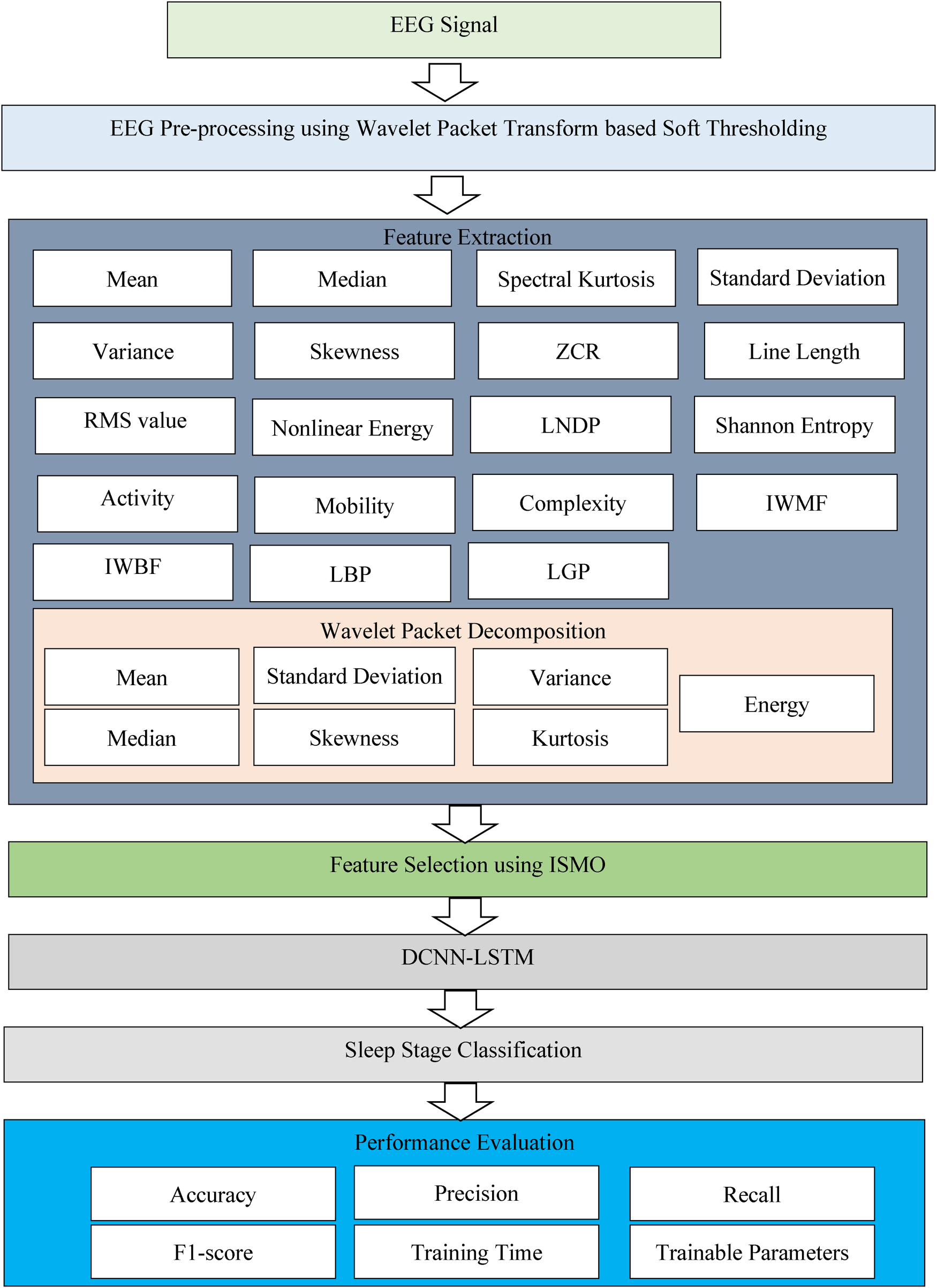
Flow diagram of WPT-ISMO-DCNN-LSTM-based SSC scheme.
Further, the EEG signals’ spectral and temporal features are extracted to characterize them. 513 features are extracted using spectral and temporal feature extraction techniques. It uses ISMO to select the prominent features from the available feature set. The system's performance is validated for the set of different features selected using ISMO. Afterwards, light-weight DCNN-LSTM is introduced for the six sleep stages, including waking, REM, N1, N2, N3, and N4. The DCNN provides the spatial and hierarchical features, and the LSTM provides temporal features and long-term dependencies in the features. The outcomes of the suggested system are estimated based on accuracy, precision, recall, F1-score, training time, and total trainable parameters.
The representation capability of the EEG signal can be improved using various time-domain, frequency domain, and textural features. Combining spectral, temporal, and texture features of EEG enhances sleep stage classification by capturing complementary information. Spectral features help distinguish sleep stages based on characteristic rhythms, temporal features capture dynamic changes over time, and texture features provide structural insights into EEG patterns. Intensity-weighted mean frequency (IWMF), Intensity-weighted bandwidth (IWBF), Wavelet Packet Transform (WPT), Energy, etc, represent frequency domain features as described in Table 1. The mean, median, variance, kurtosis, zero Crossing Rate (ZCR), standard deviation, activity, mobility, complexity, line length, Shannon Entropy, non-linear energy, etc are the time domain features. However, Local Binary Pattern (LBP), Local Neighbor Descriptive Pattern (LNDP), and Local Gradient Pattern (LGP) depict textural features. The features set is provided to the feature selection algorithm, and selected prominent features are provided to the DCNN algorithm. Combining multiple features improves the feature representation capability and helps minimize the computational complexity of the DCNN algorithm.
EEG Multiple Feature Details.
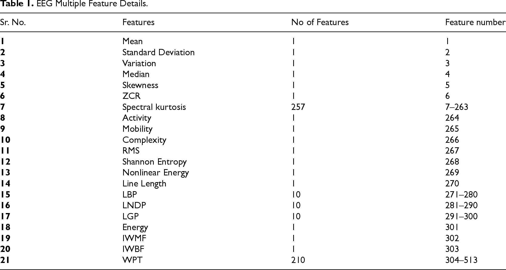
EEG Multiple Feature Details.
Mean, Standard Deviation and Variance
The influence of different sleep stages is analyzed through various time-domain, frequency-domain, and textural features of EEG signals. The mean and standard deviation capture amplitude variations over time, while variance reflects the consistency of the EEG signal. Equations 1–3 describe the mean (μ), standard deviation (σ), and variance (vr) for an EEG signal E with N samples.
Hjorth's Parameters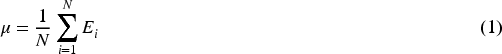


Activity (act), mobility (mob), and complexity (com) quantify energy, oscillations, and intricacy in EEG patterns. Activity is higher during wakefulness and lower during sleep, similar to variance. Mobility is defined as the ratio of the variance of the first derivative of the EEG signal to the variance of the EEG signal. Complexity is calculated as the ratio of the mobility of the first derivative of the EEG signal to the mobility of the EEG signal. Equations 4–6 are used to compute act, mob, and com, respectively.
RMS


The root mean squares of the amplitudes of the EEG samples ZCR
ZCR reflects the noisiness in the EEG caused by amplitude transitions. RMS measures the overall signal power, while entropy captures random or irregular patterns in the EEG. In Equation 8, 1{.} provide 1 value that indicates a zero crossing, signifying a change in the sign of the current samples compared to the previous ones. The sign of the EEG samples is determined using the sign function.
Line length (LL)
The LL of the EEG offers the overall vertical length or curve length which depicts the sleep pattern in the EEG signal. The line length is employed to compute the fractal dimensions of discrete wavelet transform coefficients of the EEG. The LL is computed using equation 9.

Energy (EN)
Energy represents the strength of the signal across different frequency bands, reflecting arousal levels during transitions between lower and higher sleep stages. The Energy (EN) is calculated using equation 10.
Instantaneous Wavelet Moment of Frequency (IWMF)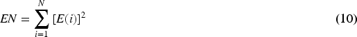
The IWMF offers dynamic disparities in EEG that portray micro-arousals and sleep spindles. The IWMF is calculated using equation 11 where E[k] is normalized PSD at frequency f[k].
Instantaneous Wavelet Bandwidth of Frequency (IWBF)
IWBF quantifies the bandwidth of sleep frequency bands, as defined in equation 12. This measure is crucial for differentiating between REM and non-REM sleep stages. The PSD tends to show higher values during periods of wakefulness and REM sleep.

The Local Binary Pattern (LBP) features capture the local temporal variations in EEG signal patterns. The Local Neighborhood Difference Pattern (LNDP) highlights finer amplitude variations, micro-arousals, and transient changes across different sleep stages. LBP, converts the partial time series data to encoded patterns. Meanwhile, the Local Gradient Pattern (LGP) detects directional changes in EEG signals, offering insights into both pronounced and subtle variations, such as those occurring during sleep K-complexes and spindles. LGP measures EEG gradients (G) as represented by an equation, where c represents the central value in the window, and Wavelet Packet Transform (WPT)


WPT offers the stationary and transient patterns of the EEG in the time-frequency domain. The EEG is decomposed using a “db2” filter up to 5 levels that split it into different sub bands to analyze the spectral changes in each sub band. The EEG signal has maximum frequency of 100–150 Hz, therefore we have decomposed the signal up to 5 level to analyze the low frequency sub bands. WPT enables complex information such as voice, pictures, EEG signals, music, emotion, and patterns to be broken into fundamental forms at a variety of places and scales, and then reconstructed with a high level of accuracy. WPT assists in the analysis of the variance that occurs throughout the course of sleep as a result of the various sleep patterns.
Figure 2 represents the three level where
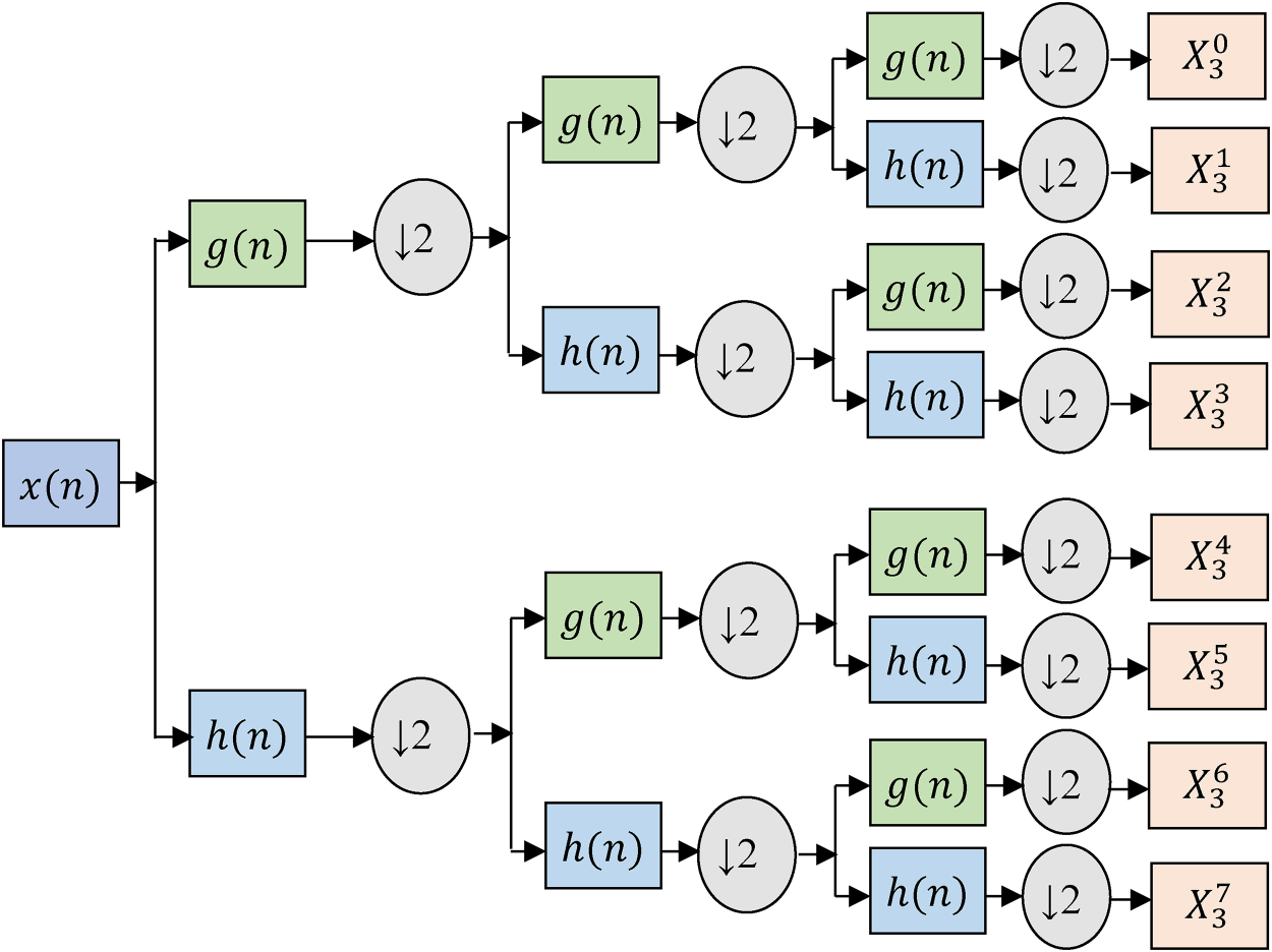
WPT decomposition of EEG up to 3 levels.
As indicated in Equation 16 and 17, the Daubechies (db2) wavelet is employed at different scales in order to decompose the wavelet packet basis function 

Where 

The EEG signal is separated into segments at level j using Equation 20.

Where, 
The wavelet coefficient 
Equation 23 gives a distinct WPT set for L level.

By using a db2 filter, the EEG signal may be divided into five levels. Seven statistical variables, including the mean, median, standard deviation, variance, skewness, and kurtosis of each wavelet packet, are retrieved for the last level of decomposition. The various elements of the WPT give the spectrum variations that occur in the EEG signal as a result of changes in the distinct waves that make up the sleep pattern. There is a total of 210 WPT characteristics produced as a consequence of the five-level decomposition of the speech signal.
Various EEG feature selection schemes has been presented in recent years for choosing the crucial attributes of EEG depicting the sleep variations. However, the traditional optimization algorithms suffer from poor balance in exploration and exploitation, poor solution diversity, lower search space, and inferior convergence. To tackle these challenges, this work provides an ISMO for improving the performance of optimization algorithms based on feature selection (Agrawal et al., 2018, Garip et al., 2024; Houssein et al., 2024). ISMO selects the important features from the spectral and temporal features to help minimize the computational complexity of the DCNN framework. The features are selected in groups starting from 100 up to 513. Bansal et al. (2014) have studied the spider monkey method, also known as SMO, for multi-objective numerical optimization and metaheuristic problem-solving. Figure 3 depicts the flow chart for the planned ISMO.
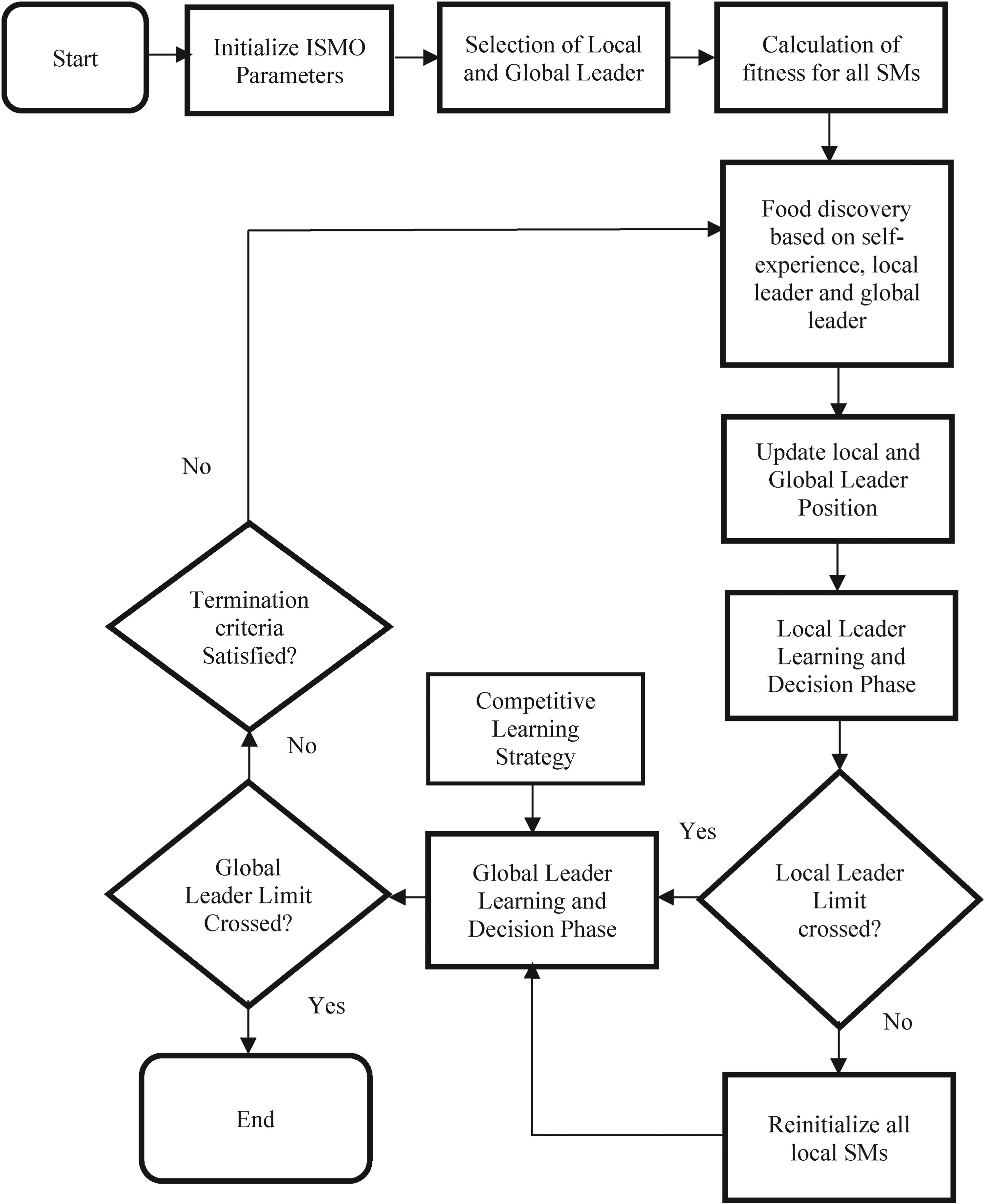
Flow chart of ISMO for feature selection.
As a member of a fission-fusion society, the spider monkey lives in a group of 40 to 50 individuals, and most animals live in groups of 40 to 50 individuals that may be managed by an adult female known as the global leader. The hunt for food falls within the purview of the dominant world power. When they cannot find enough food, they divide the primary group into many subgroups, each consisting of three to eight monkeys so that they may search for food sources independently. Every subgroup has a local group leader accountable for route discovery, planning, and decision-making. Spider monkey's food discovery strategy includes four stages. The improved ISMO considers a competitive learning strategy for exploring the new population in case of the stagnation of the elite group.
The first stage deals with beginning of food discovery and evaluation of distance of home place from food source. The second stage consists of communication and updating of position and distance information with local leader and group members. In third stage, the local leader decides best position of subgroup and if the position gets unchanged for stipulated time, then all subgroup members decide to forage the food in diverse way independently. In final stage, the global leader decides the finest position of food source with the help of information gathered from local leaders. The global leader divides the groups in small groups if stagnation occurs for particular group (Bansal et al., 2014; Sharma et al., 2019). The traditional SMO sometimes fails to provide the optimal solution if the local groups fail to provide the expected solution and often results in stagnation. ISMO provides additional decision in global leader decision phase to minimize the stagnation. The global leader provides the fusion of two groups in case of stagnation by replacement of weak members of one group with strong members of another group. This strategy is useful in case any group member gets abandoned or continuously provides constant inferior fitness.
Initialization Phase
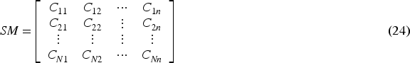
The initialization phase consists of generation of M spider monkey (SM). The initial population includes N subgroups for food foraging (finding optimal feature set) where each subgroup encompasses members to indicate optimal channel value. The spider monkey population is given by equation 24.
Here Fitness Function
The fitness function of the ISMO based feature selection scheme depends upon interclass variability (
The intra-class variability represents the closeness in same class channel information whereas interclass variance depicts the distinctiveness of two classes. The intra-class and interclass variability are computed using equation 26 and 27.


Where Local Leader Phase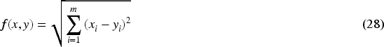
The local leader of group updates the positions of spider monkeys (SMs) using experience of local leader and members. If the fitness of new SM is inferior to previous local leader solution, then SM updates its position using equation 29.

Where Global Leader Phase
The global leader modifies the position of SMs and subgroups based on the experience of global and local leaders and probability fitness using equations 30 and 31.
Global Leader Learning Phase

The global leader updates the position of SM based on the best fitness value among all groups using a greedy selection scheme.
Local Leader Learning Phase
The local leader updates the position of SM based on fitness value in individual local groups using a greedy selection scheme. However, the SM with the highest fitness value is chosen as the local leader.
Local Leader Decision Phase
In case of stagnation, all individual SMs of local groups modify their position arbitrary using decision of local and global leader using equation 32.
Global Leader Decision Phase
The global leader divides the group in smaller groups when global leader position remains unchanged for given time and maximum iterations. If large groups formed are deprived of modifying global leader position, then global leader combines the entire group in single group which is known as fission and fusion strategy.
Competitive Learning Strategy
The competitive learning strategy is utilized to improve the exploitation of the SMO which minimizes the stagnation in SMO population. The elite groups are considered which are having immediately lesser fitness value than the global best. The competitive strategy considers the replacement of feeble monkeys which leads to the lower fitness value by strong monkeys to get better fitness of the overall local group. The member with higher feature variance is considered strong members. The global leader is replaced by new population generated by a competitive strategy if the competitive learning strategy provides the population with better fitness. The suggested strategy is evaluated at every iteration which helps better reuse of the spider monkey group for getting optimal fitness. The algorithm of the competitive learning strategy of the spider monkeys is described as follows:
The DCNN is used for providing the spatial connectivity, local and global correlation in different EEG features to depict the complex sleep patterns. The LSTM assist to offer superior temporal dependency and long-term temporal depiction of the EEG signals. The combination of DCNN and LSTM helps to improve the feature depiction of EEG signals (Bhangale and Mohanaprasad, 2024a). The suggested lightweight DCNN consists of three convolution layers, three rectified linear unit (ReLU) layers, three batch normalization layers (BN), a fully connected layer (FC) and softmax classifier layer. The DCNN is followed by two LSTM layer having 20 hidden layers to enhance the temporal and long-term representation of the EEGs (Bhangale and Mohanaprasad, 2024b). The framework of the DCNN-LSTM is given in Figure 4. The DCNN includes three layers of CNN with 64, 128 and 256 filters at first, second and third layer respectively.
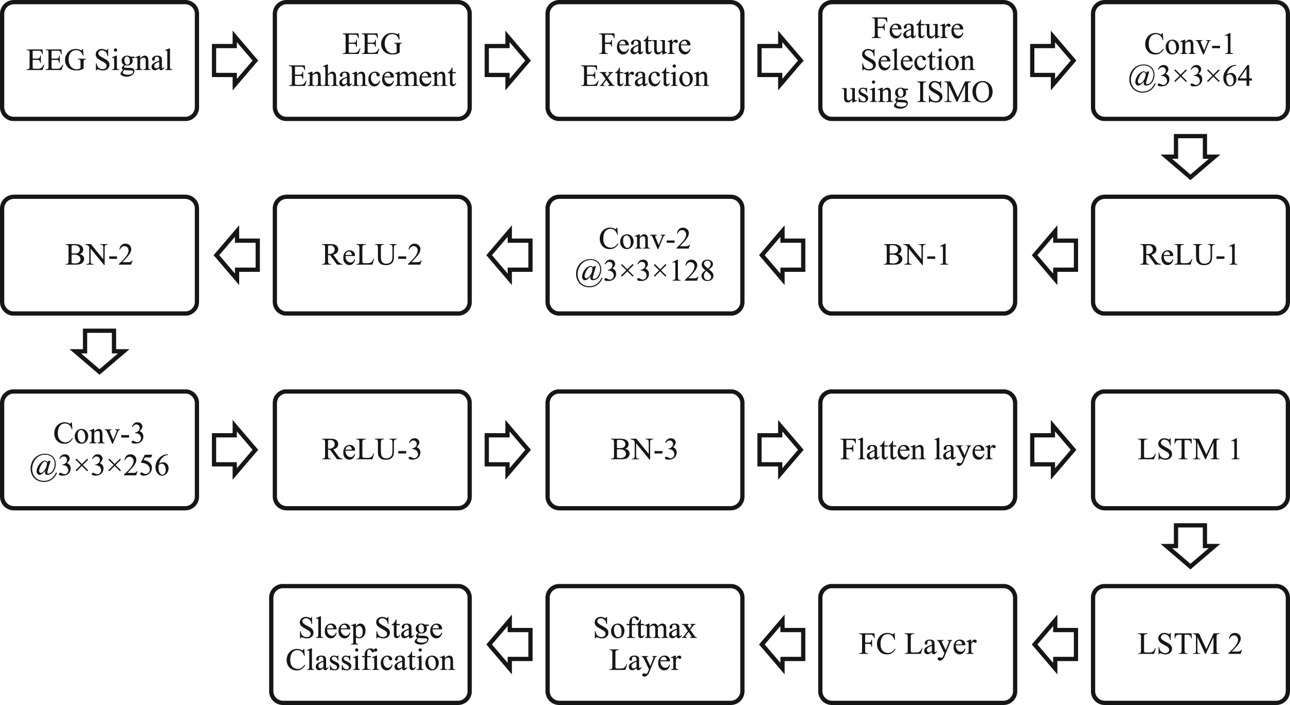
Framework of DCNN.
The DCNN accepts the one-dimensional set of features selected using SMO algorithm. The convolution layer provides the correlation between different features of the EEG signal. It enhances the representation capability of the features and provides the connectivity between different local and global features of the EEG signal. It uses convolution filter with 

The Batch normalization standardizes the features. The flattening layer converts the feature to a 1-D vector. Then, 2 LSTM layers with 20 hidden layers are considered. LSTM includes various memory cells, so four stages exist in updating cell state.


Here, 


Where
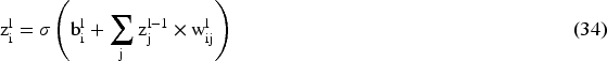
The FC layer connects every neuron and provides the connectivity between deep features. Lastly, the softmax classifier provides the probability of the predicted class for SSC.
The WPT-ISMO-DCNN-LSTM scheme is simulated on MATLAB 2020b on a computer with 20GB RAM and the Windows operating system. The performance of the WPT-ISMO-DCNN-LSTM-based SSC scheme is evaluated on the sleep-EDF dataset. The outcomes are estimated using accuracy, recall, precision, F1-score, trainable parameters, and training time. The DCNN is trained using the Adam optimization algorithm with an initial learning rate of 0.001, a cross-entropy loss function for 100 epochs. It achieves 100% training accuracy for 100 epochs. The training accuracy and loss of the proposed SSC for the 6-class SSC are given in Figure 5.
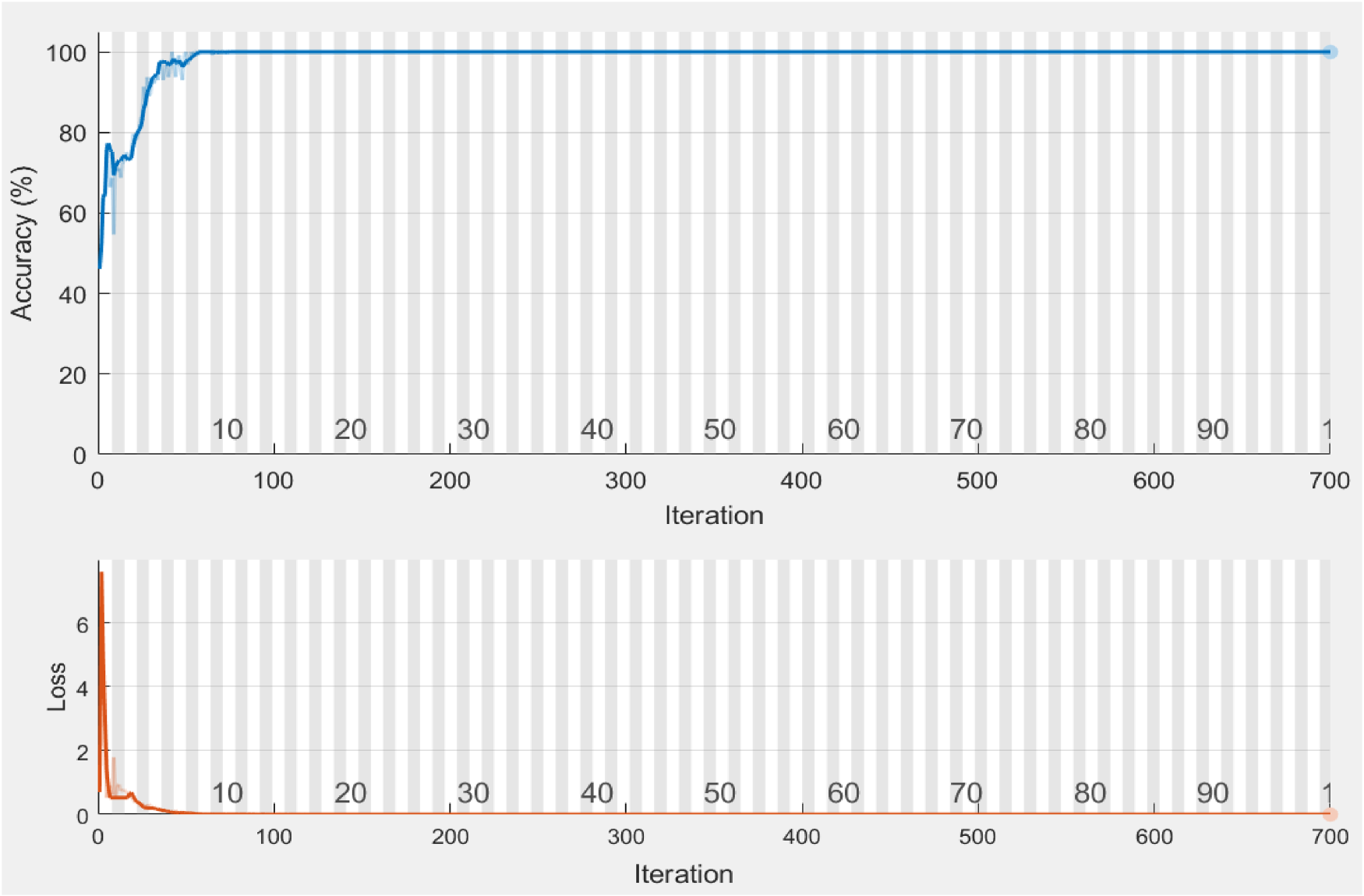
Training accuracy and loss of DCNN for 6-class SSC.
The sleep EDF datasets used in this study are publicly accessible at https://www.physionet.org/content/sleep-edfx/1.0.0/. It is a freely accessible Physio Net sleep-EDF extended dataset with PSG data from 197 individuals. For the suggested SSC, a single-channel EEG signal with a frequency of 100 Hz was used. The signals are chopped into 30-s samples using the Polyman Tool and the hypnogram for sleep stage labeling. The samples are divided into six sleep stages, including four sleep stages (S1, S2, S3, and S4), rapid eye movement (REM), and wake stage (W). We have considered 1000 samples of each class with single-channel EEG from Pz-Oz (Parietal-Occipital region) for the experimentation. The dataset is split in a ratio of 70:30% for the system's training and testing. The training dataset consists of 4200 samples, and the testing dataset includes 1800 samples.
Discussions on Results of ISMO-Based Feature Selection for SSC
Figure 6 shows the selected features using SMO for different numbers of features. It shows that WPT, Kurtosis, LBP, LGP, Standard deviation, mean, median, skewness, variance, and LNDP are more important in the feature set and are ranked higher. Kurtosis, WPT, and LBP features are available in every feature selection strategy. It is also noted that the local features, such as Kurtosis, WPT, LBP, LNDP, and LGP, show more distinctiveness compared with global features, such as mean, median, ZCR, etc. The kurtosis, WPT, and EEG texture features show better variations over the local region of the EEG signal. The performance of the WPT-ISMO-DCNN-LSTM-based SSC scheme for 6-stage SSC is compared with and without pre-processing of the signal and feature selection. It is observed that pre-processing and feature selection help achieve better classification accuracy.
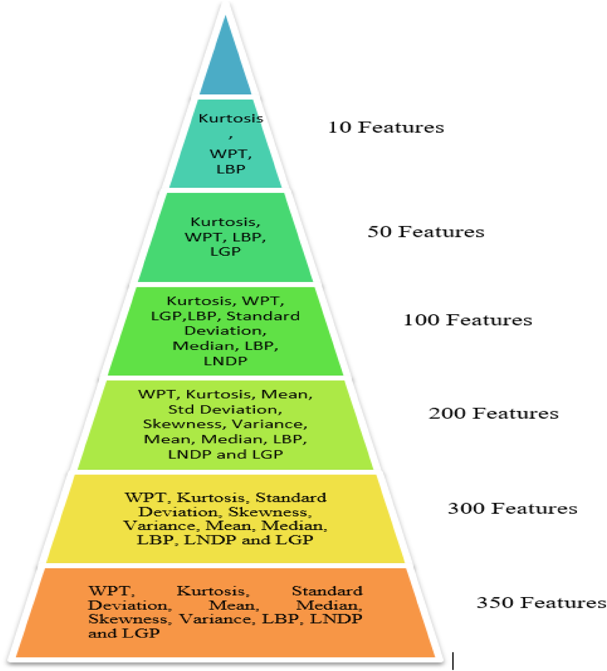
Ranking of selected features using SMO.
The DCNN provides an accuracy of 92% for all features without feature selection and pre-processing of the raw EEG signal. The WPT-based EEG enhancement leads to an improvement in the accuracy of the 6-stage SSC to 93%. The SMO-based feature selection results in an accuracy of 95% without preprocessing of the EEG signals. Meanwhile, WPT-SMO-DCNN provides an accuracy of 98% for the 6-stage SSC. The WPT-SMO-DCNN provides a precision of 0.99, a recall of 0.98, and an F1-score of 0.98. The confusion matrix for the 350 features for the 6-class SSC is shown in Figure 7. It provides the accuracy of 100% for wake, 97.7% for S1 stage, 99.3% for S2 stage, 99.3% for S3 stage, 98.7% for S4 stage, and 99% for REM for the 6-class SSC. The accuracy, precision, recall, and F1 score of the WPT-ISMO-DCNN-LSTM-based model are provided in Figures 8–11, respectively.
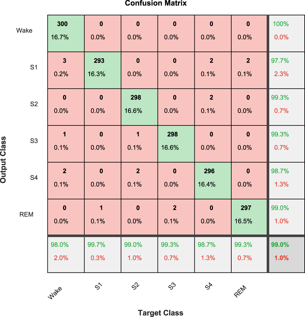
Confusion Matrix for 6-stage SCC for 350 features.
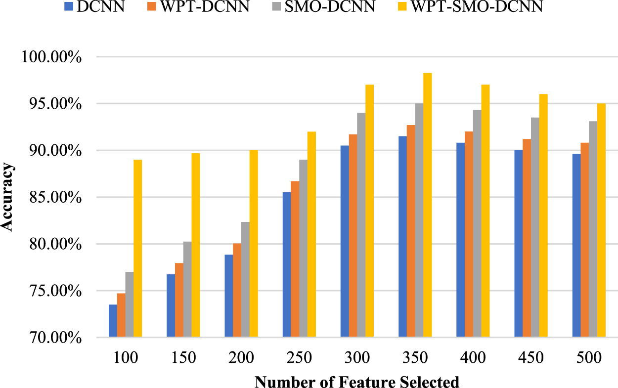
Accuracy of suggested SSC for different features.
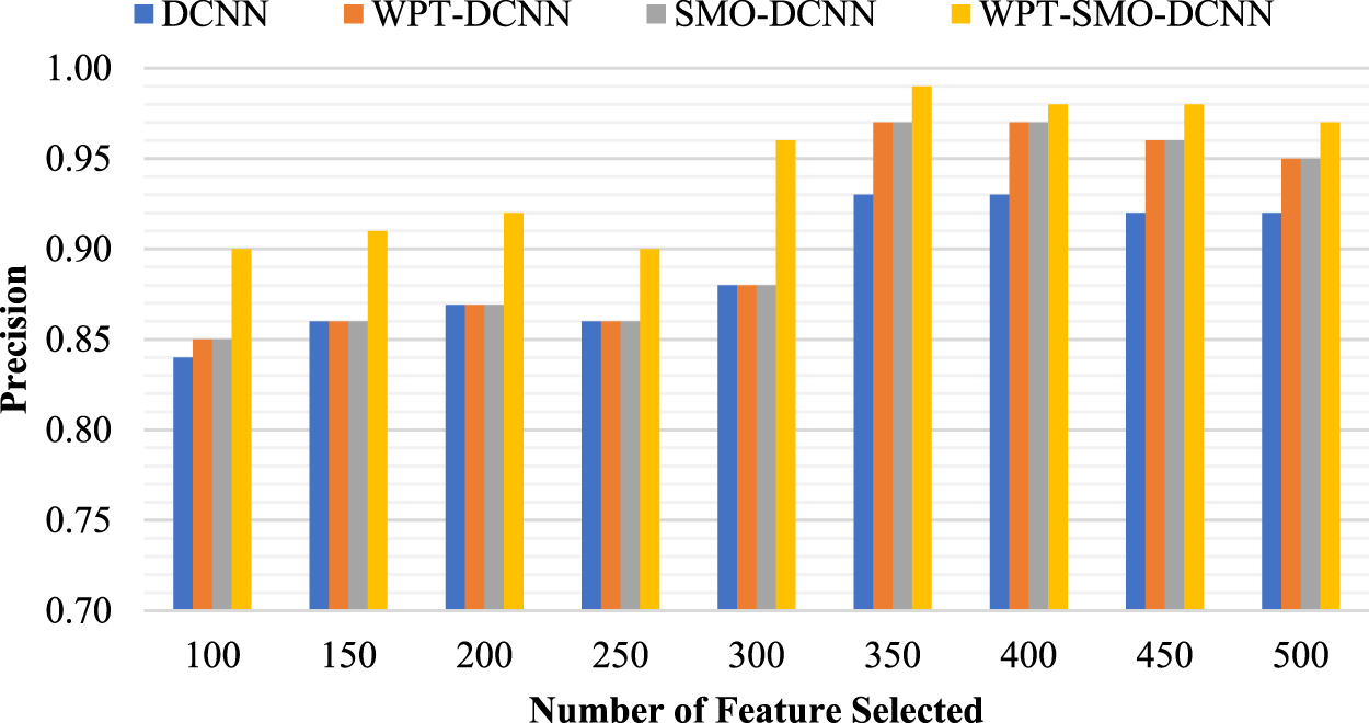
Precision of suggested SSC for different features.

Recall of suggested SSC for different features.

F1-score of suggested SSC for different features.
The WPT-DCNN-LSTM provides accuracy of 89% for 100 features, 89.70% for 150 features, 90% for 200 features, 92% for 250 features, 97% for 300 features, 99% for 350 features, 97% for 400 features, 96% for 450 features and 95% for 500 features with improved SMO. The WPT-DCNN-LSTM provides the 95% accuracy for the feature selection using traditional SMO. The WPT-SMO-DCNN provides an accuracy of 0.98 for 350 features, which is superior to all features (0.95). It is noted that increasing features from 100 to 350 shows a significant rise in accuracy; however, beyond 350, it shows a reduction in accuracy.
The effectiveness of the WPT-ISMO-DCNN-LSTM-based SSC for different CNN layers is described in Table 2. It shows better accuracy for a three-layer DCNN architecture, lower trainable parameters, and a significant decline in training time. The suggested scheme provides an accuracy of 0.99, precision of 1, recall of 0.99, and F1-score of 0.99 for 3 CNN layers. The 3-layered architecture provides ∼5.9 M trainable parameters and training time of 498 s The CNN with one and two layers offers accuracy of 91% and 97% for 6-class SCC and provides the highest accuracy of 99% for 3-layered DCNN-LSTM. For a higher number of CNN layers, the accuracy shows a slight decline and a vast boost in trainable parameters and time, which decreases the implementation flexibility of the system for real-time applications. Therefore, we have selected a 3-layered DCNN along with LSTM for SCC. When the performance is evaluated based on the Fredman test, then it provides a t-statistic value of −6.35 and a p-value of 0.0032, depicting that WPT-ISMO_DCNN-LSTM outperforms WPT-ISMO_DCNN.
Accuracy of Different CNN Layers.

Accuracy of Different CNN Layers.
The results of the recommended procedure are estimated for different phases of sleep. The experimental results are analyzed for the five groups as given in Table 3. For the 2-class classification, the model is trained for wake vs all sleep stages, such as (S1, S2, S3, S4, REM). The 3-class classification considers wake (S1, S2, S3, S4) and REM stages. The 4-class includes wake, S1, S2, (S3, S4) and REM stages. The 5-class group encompasses wake, S1, S2, S3, S4, and S5 stages. Consideration of different classes for the sleep stages is needed to analyze the system's robustness for determining the complex sleep patterns in higher classes. It helps to analyze the transition from one sleep stage to another to determine the mental and sleep state of the person.
Different Classes for Sleep Stage Analysis.
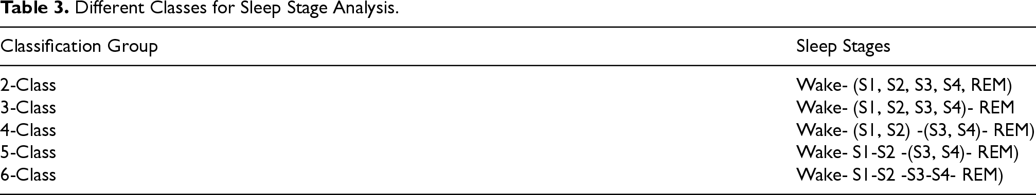
Table 4 shows the outcomes of the proposed ISMO-based feature selection compared with the traditional SMO, genetic algorithm (GA) (Shon et al., 2018), and particle swarm optimization (PSO) (Sun et al., 2022) - based feature selection for 350 features. The GA achieved a consistent performance with an accuracy, precision, recall, and F1-score all at 0.92, indicating reliable but moderate optimization. PSO showed improved results over GA, especially notable in the recall (0.97) and F1-score (0.95), highlighting better sensitivity towards correctly identifying sleep stages. SMO further enhanced the performance with a significant jump, achieving 0.95 accuracy and exceptionally high precision (0.97) and recall (0.98), leading to a strong F1-score of 0.97. The ISMNO provides improved accuracy of 99% over the SMO (95%), PSO (93%), and GA (92%). It also boosts the recall and precision of the SSC system.
Different Classes for Sleep Stage Analysis.

The SSC results of the WPT-SMO-DCNN are compared with the previous state-of-the-art for SSC, as given in Table 5. The WPT-ISMO-DCNN-LSTM-based approach performs better than the previous state-of-the-art sets for 4-class, 5-class, and 6-class sleep stage classification. The WPT-ISMO-DCNN-LSTM-based approach has significantly improved over traditional SSC approaches, as the multichannel signals describe prominent information on sleep stages. The WPT-ISMO-DCNN-LSTM provides improved accuracy of 99% over WPT-SMO-DCNN (98.30%), 1-D CNN (91%), AdaBoost-RF (91.55%), CareSleepNet (87.9%), and RNN (88.47%) for 6-class SSC. It provides enhanced 99.33% accuracy compared with WPT-SMO-DCNN (97%), separable CNN (85.22%), 1-d CNN (91.22%), RNN (90.30%), CNN-fine grain (92.20%), encode-decoder (88.9%), and Bootstrap Aggregating (86.53%) for 5-class SSC. For 4-class SSC, the WPT-ISMO-DCNN-LSTM gives 98.50% accuracy, which has shown noteworthy improvement over WPT-SMO-DCNN (97.30%), 1-D CNN (92.36%), and RNN (91.93%). It provides 98.50%, 97.30%, and 94.64% accuracy for WPT-ISMO-DCNN-LSTM, WPT-SMO-DCNN, and 1-D CNN, respectively, for 3-class SSC. The WPT-ISMO-DCNN-LSTM provides an accuracy of 99% for 2-class SSC, 99.70% for 3-class SSC, 98.50% for 4-class SSC, 99.30% for 5-class SSC, and 99% for 6-class SSC for 350 features. When the performance of the suggested method is compared with the SMO-based feature selection, the ISMO helps to provide better prominent features and leads to higher accuracy than the SMO-based feature selection scheme. Additionally, we have analyzed the effectiveness of the proposed algorithm based on Kohen's Kappa. The WPT-ISMO-DCNN-LSTM offers the Kohen's Kappa rate of 0.9878, 0.9921, 0.9853, 0.9967, and 0.9828 for the 6-class, 5-class, 4-class, 3-class, and 2-class SSC.
Performance Comparison with the Previous Techniques.

Performance Comparison with the Previous Techniques.
The comparative accuracy analysis across multiple sleep stage classification (SSC) methods shows that the WPT-ISMO-DCNN-LSTM model consistently outperforms traditional and state-of-the-art techniques across all classification levels. It achieves the highest accuracy of 99.00% in 2-class and 6-class SSC, and up to 99.70% in 3-class classification. The second-best performance is from the WPT-SMO-DCNN, reaching 98.54% in 2-class and 98.30% in 6-class SSC. Traditional methods like RNN, 1-D CNN, and Bagging exhibit notably lower accuracies, especially in more complex classifications like 5-class and 6-class. Several models, such as CareSleepNet, Encoder-Decoder, and AdaBoost-RF, do not surpass 92%, highlighting the significant improvement the proposed WPT-ISMO-DCNN-LSTM approach offers. Overall, the results demonstrate the superior performance and robustness of the proposed hybrid model for fine-grained SSC tasks.
The proposed WPT-ISMO-DCNN-LSTM-based SSC model has significant healthcare implications. Achieving up to 99% accuracy across 6-stage sleep classification enhances the precision of diagnosing sleep-related disorders. The integration of WPT for EEG enhancement and ISMO for feature selection allows for accurate classification with reduced computational complexity and training time. This makes the model suitable for real-time and embedded healthcare systems. Its ability to analyze multiple sleep stages supports a deeper understanding of sleep transitions, aiding in diagnosing neurological and psychological conditions. The high precision, recall, and F1-score ensure minimal false positives and negatives, which is critical for patient safety. Additionally, its compatibility with raw EEG signals simplifies implementation with wearable devices for home-based monitoring. The suggested SSC provides superior accuracy for the 6-class SSC than the existing method. It minimizes the computational complexity and time of the system using ISMO-based feature selection that assists in choosing prominent features. The multiple EEG features assisted in capturing the spectral, time-domain, and sleep pattern features to increase the feature depiction. However, the outcomes are limited for the real-time system because of the availability of diverse patient data and poor interpretation capability.
Conclusion
This paper presents SSC based on multiple EEG features, ISMO-based feature selection, and DCNN-based sleep stage classification. The Multiple EEG features describe the EEG signal's spectral, time domain, and spatial properties to describe the complex sleep stage pattern. The WPT is used to minimize the noise and artifacts present in the EEG signal. The ISMO-based feature selection helps to select the crucial features that decrease the computational intricacy of the DCNN-LSTM. It assists in improving the diversity of solutions and search space and provides a balance between exploration and exploitation compared to traditional SMO. The DCNN-LSTM offers better connectivity, correlation, long-term dependency, and temporal depiction of the single-channel EEG for the SSC. The ISMO algorithm selects the prominent features from the existing ones. The WPT-ISMO-DCNN-LSTM resulted in the overall accuracy of 99% for 2-class, 99.70% for 3-class, 98.505% for 4-class, 99.30% for 5-class, and 99% for 6-class sleep stage classification.
In the future, more focus can be given to improving the explainability of the deep learning framework and minimizing the computational time of the overall system. Using multiple modalities can improve the effectiveness, security, robustness, and reliability of the SSC scheme. The proposed scheme can be utilized for sleep disorder detection.
Footnotes
Ethical Approval
Not applicable.
Funding
The authors received no financial support for the research, authorship, and/or publication of this article.
Declaration of Conflicting Interests
The authors declared no potential conflicts of interest with respect to the research, authorship, and/or publication of this article.
Data Availability
The data can be made available on reasonable request to the authors.