



Abstract
The building sector is one of the most developed areas within countries due to its contribution to economic growth. On the other hand, the building sector is increasingly depleting energy resources, making it necessary and urgent to reduce its consumption. In this context, we deal with the issue of energy consumption of residential buildings, by studying and discussing energy consumption forecasting models for residential buildings to improve building designs and enhance energy efficiency. To achieve these objectives, it is necessary to explain the behavior of forecasting systems. This will enable stakeholders to make informed decisions. In the context of explainable artificial intelligence, which provides an interactive interface for stakeholders to interact with intelligent systems, check their results, and trust their behavior; we present a fuzzy prediction model based on subtractive clustering and linguistic hedges to forecast energy consumption for residential buildings. The model is tested on a dataset containing 768 residential building information with eight input and two output variables. The proposed model is compared with Elastic Net, Random Forest, MLP, Linear Regression, Gaussian Process Regressor, ExtraTrees, Decision Tree, KNeighbors, SVR, Adaboost, XGBoost, and Gradient Boosting Regressor. The simulation findings show the efficacy of linguistic fuzzy rules in the forecasting of residential energy consumption. In parallel with prediction, the model provides a good balance between interpretability and accuracy.
Keywords
Introduction
In short, medium, and long term, all government policies are directed at energy because they have a positive effect on society and the environment. Therefore, countries finance energy projects with huge budgets. In addition, the construction industry is one of the largest consumers of energy, especially for residential purposes. As a result, countries have accelerated measures to limit growing energy consumption. Simple procedures can be used to greatly reduce power consumption, such as unplugging unused appliances, avoiding wasting hot water, and encouraging the use of energy-saving appliances. Regarding the buildings sector, it is possible to improve the use of energy systems, such as cooling and heating loads, control systems and surveillance systems. These procedures require prior knowledge of energy requirements, especially heating and cooling loads. Forecasting heating and cooling loads helps in determining the structures of buildings to be constructed, reducing electricity consumption, and constructing intelligent buildings. The energy forecast can be classified into three types: electric load, heating load and cooling load. The importance of forecasting heating and cooling loads is to design energy efficient buildings, improving the performance of air conditioning systems, and reducing electricity consumption. In this regard, energy demand is affected by the thermal behavior of the building due to the interweaving of many different factors such as weather conditions, building quality, energy usage patterns and human behavior, etc. In order to overcome these challenges, several methods have been used in the prediction process, such as machine learning, physical and statistical methods. The physical methods are based on the use of physical simulation software to model thermal behavior. Several simulation programs have been developed to determine the energy balance, such as EQUEST; Using these programs requires high cost and sufficient experience. Statistical methods are based on the collection of training data to implement mathematical functions that define the linear relationship between input and output variables. But this type of statistical method is not precise enough because it is not compatible with the nonlinear behavior of energy demand. Machine learning methods provide precise, scalable, and stable solutions to solve problems caused by uncertain or missing data. Many researchers have studied the energy consumption prediction of residential buildings (Zhou et al., 2020), (Li et al., 2020), (Amasyali & El-Gohary, 2018). In 2011, YILDIZ and GERS examined the key elements affecting the heating and cooling of buildings in hot and humid environments by analyzing the structure of apartments (Yildiz & Arsan, 2011). YANG used LS-SVM (Least Square Support Vector Machine), he compared SVM to ANN using backpropagation learning algorithm (Yang et al., 2014). The SVM performs better than ANN in reducing the value of mean absolute percentage error (MAPE) and (coefficient of determination). In (Sholahudin & Han, 2015), SHOHUHUDIN and HWATAIK demonstrated the feasibility of using machine learning methods to predict instantaneous heating loads to optimize building energy consumption in winter. ANN is widely used in situations where even nonlinear assumptions fail to learn; In 2016 KHAYATIAN et al. used ANNs to forecast building energy demand based on the energy consumption of existing buildings by considering simple variables (Khayatian et al., 2016). CHENGDONG proposed a new deep learning model to predict the energy demand of buildings (Li et al., 2017). The proposed method has shown better prediction performance in various situations of Energy Consumption Prediction of Residential Buildings. It should be noted that the ANN models are the most used in energy forecasting applications in buildings because they have shown better performance than physical and statistical methods.
As is well known, ANN models belong to the more complex models that can be difficult to debug, understand, and control; thereby impeding their adoption. However, in order to make informed decisions, it is necessary to explain the system's predictions to the stakeholders (Arrieta et al., 2020). As shown in Figure. 1, at a high level, there are three stakeholder groups for machine learning systems that drive the dual aims of model understanding and providing human interpretable explanations to different stakeholders in order to build trust. For engineers building models, the focus is more on interpretable machine learning techniques for model understanding and improving model performance. Conversely, trust is key for model consumers who are looking to understand the impact of model predictions more than the model internals. The role of regulators is to ensure model decisions are in compliance with laws and do not amplify undesirable bias from underlying data sets.

Model understanding for different stakeholders.
Understanding a model's behavior is critical to many tasks: – Explain predictions to support decision making processes – Debug unexepted behavior from model – Refine modeling and data collection processes – Present the model's predictions to stakeholders.
To complete these tasks, it is important to apply XAI explanatory techniques,such as (SHAP, LIME, CONTRAFACTUAL, ANCRE), to opaque models or building an interpretable model with a good balance between accuracy and interpretability (Belle & Papantonis, 2020). In the literature, there are many machine learning interpretability methods, Figure. 2 shows a taxonomy of these methods. Post hoc or intrinsic, this criteria distinguishes whether interpretability is achieved by restricting the complexity of machine learning model, known as intrinsic, or by applying methods that analyze the model after training, known as post hoc. Intrinsic interpretability refers to machine learning models that are considered interpretable due to their simple structure, such as decision trees, Bayesian networks and linear models. Post hoc refers to achieving interpretability after model training. Permutation feature importance, for example, is one such post hoc interpretability method. Therefore, this is more of a considerable change in the feature space and how it affects the output of models. Local or global interpretability: local refers to whether the scope of interpretability is limited to individual predictions and or a small part of the model's prediction space.these explanations tend to provide a higher precision view, particularly of individual predictions, but lower recall understanding of a model's behavior across all examples. Global here refers to whether the interpretability scope is the entire model's prediction space. model specific or agnostic: model specific here refers to the interpretability method being restricted to usage on specific ml models due to their definition. Examples here include interpretability methods that rely upon some intrinsic part of a model's learning method,such as neural network gradients. Conversely, model agnostic interpretability methods do not rely on model internals, instead relying upon changes in input features or their values to understand how they influence the outputs of the model. Examples here include SHAP and LIME that are portable across different model types, including boosted trees and neural networks. In hybrid box on Figure 2, it's possibe to aggregate the scores of some local model-specific methods, such as sample Shapley, to provide global views of the model's prediction space using aggregations like averages and medians. Methods further differ in explanation output. Many methods return feature statistics, measuring a feature's proportional contribution to the prediction, while others extract concepts, decision rules, feature summary visualizations, counterfactual data points, or even simpler approximate models.
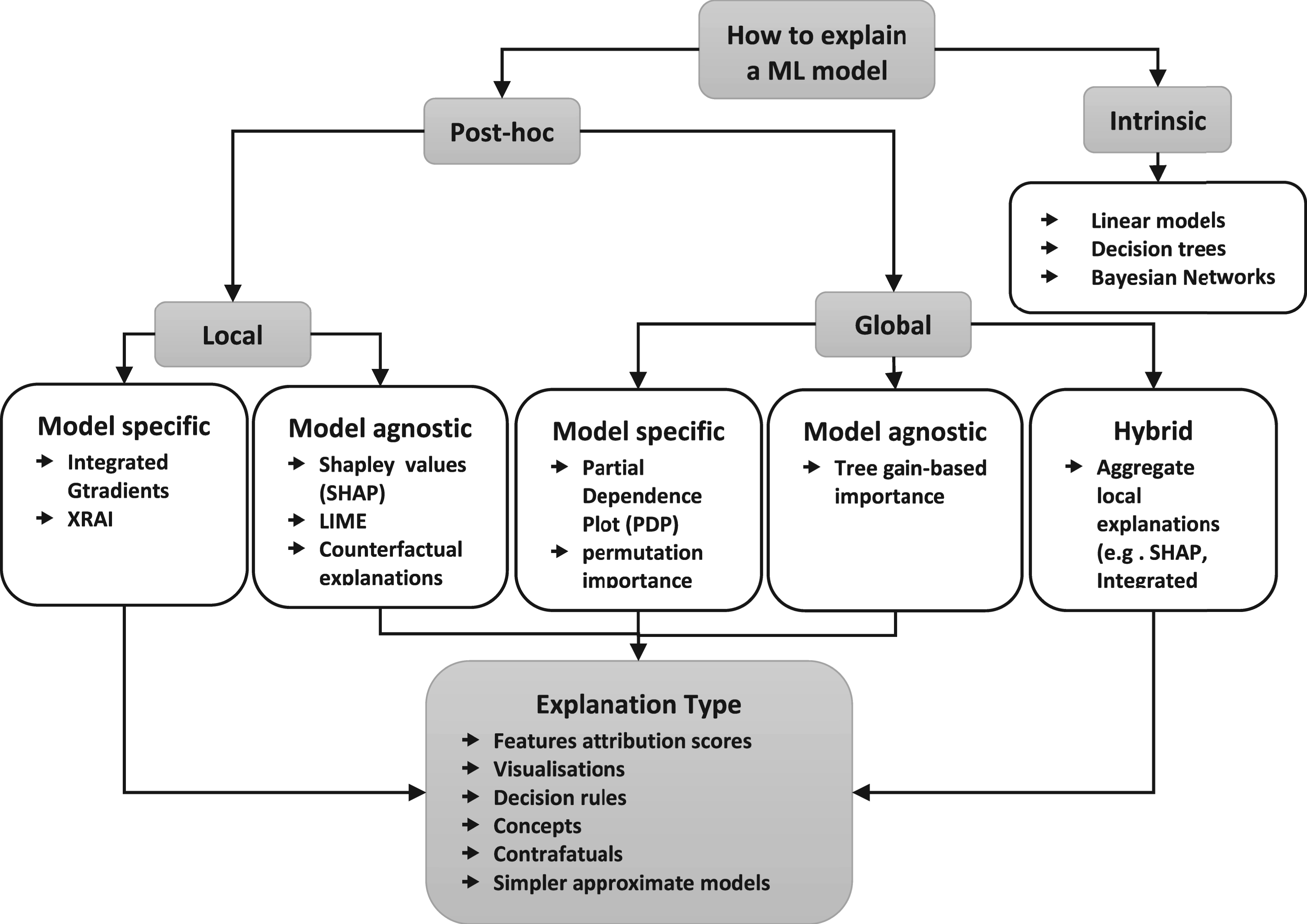
Model understanding for different stakeholders.
In this research, we put forward the need for an interpretable energy consumption prediction system of residential buildings, because the use of an interpretable system will increase the possibility of trusting the results obtained and update them in a short time with minimal effort. On the other hand, interpretable forecasting systems can communicate with users in a simple and smooth way without complex mathematical formulas, so they can contribute to the development of intelligent building systems. This need for interpretability highlights a key limitation in many existing approaches. A wide range of machine learning algorithms has been proposed in the literature, including ANN, SVM, and ensemble learning methods. However, these models often suffer from limited interpretability, making it difficult for non-experts to understand or validate predictions. Recent research has highlighted the need for models that combine high predictive accuracy with interpretability, particularly in building energy forecasting. While methods like neural networks and ensemble learning often achieve strong performance (Abdel-Jaber & Dirks, 2024), (Khastar et al., 2025), they typically require post-hoc explanation techniques such as SHAP or LIME (Abdel-Jaber & Dirks, 2024), (Shajalal et al., 2024), which add complexity and may be difficult for stakeholders to understand. This reinforces the importance of developing models that are both accurate and intrinsically interpretable, without relying on external interpretability tools (Abdel-Jaber & Dirks, 2024), (Salami et al., 2023).To address this challenge, our choice to explore fuzzy rule-based systems stems from their ability to provide interpretable and transparent decision-making processes, while maintaining reasonable predictive performance. To this end, we aim to establish a fuzzy rule-based system (FRBS) for the prediction of heating and cooling loads with high accuracy and interpretability. In this article, we propose a new method for learning linguistic fuzzy rules, which is based on subtractive clustering and linguistic hedges. These rules are used in a fuzzy system based on MAMDANI fuzzy rules, which uses the following input variables: solar energy, lighting, electrical appliances, parameters of human and heat loss due to building characteristics. The fuzzy rule-based system was proposed in (Bahani et al., 2018), which is called: Fuzzy Rule Learning through Clustering (FRLC). To evaluate the effectiveness of the proposed fuzzy rule-based model, we conduct a comparative analysis with several state-of-the-art machine learning algorithms, including Elastic Net, Random Forest, Multilayer Perceptron (MLP), Linear Regression, Gaussian Process Regressor, ExtraTrees, Decision Tree, K-Nearest Neighbors (KNN), Support Vector Regression (SVR), Adaboost, XGBoost, and Gradient Boosting Regressor. The results highlight the strong predictive performance of the proposed model. In addition to accurate forecasts, it offers interpretable fuzzy rules, making it a suitable approach for residential energy consumption modeling where both prediction reliability and model transparency are essential. To address the above research gap, this study is guided by three research questions: To what extent can a fuzzy rule-based learning system (FRLC) accurately predict heating and cooling loads in residential buildings? How effectively does FRLC provide intrinsic interpretability that enables its predictions to be understood and used by different stakeholders? Furthermore, how does FRLC perform compared to state-of-the-art machine learning algorithms in terms of both predictive accuracy and interpretability? By explicitly formulating these questions, we emphasize the dual objective of achieving high forecasting accuracy while ensuring model transparency, which is crucial for the practical adoption of energy prediction systems. The remainder of this paper is structured as follows: Section 2 presents various machine learning algorithms used to predict the heating and cooling loads of residential buildings. Section 3 details the proposed fuzzy rule-based model (FRLC). Section 4 describes the experimental setup and the performance evaluation. Finally, Section 5 concludes the paper and outlines potential directions for future research.
Machine learning is one of the important aspects of artificial intelligence. This includes the development and analysis of systems that can be able to learn from data sets, allowing devices to learn without a specifically defined program. To predict the heating and cooling loads, different building parameters on energy consumption were studied in (Li & Yao, 2020), (Moradzadeh et al., 2020), (Bourdeau et al., 2019). In this paper, the researchers studied the effect of eight parameters on heating and cooling loads, with the aim of proposing a prediction model capable of yielding results that simulate reality and explain the relationship between inputs and outputs. This interpretation is linguistic in nature, making it easier for all interveners in the building sector to understand. Figure 3 shows the general scheme for modeling building energy. As seen, the selected features for representing the building energy system are: Relative compactness (RC), roof area (RA), wall area (WA), surface area (SA), orientation (Or), overall height (OH), glazing area (GA) and glazing area distribution (GAD). The first step is the data preprocessing that includes data Cleaning, data Transformation and data Reduction. Using training dataset and machine learning algorithm, the next key stage trains and optimizes the predicting model. The final step in the learning stage is to evaluate the trained model using the testing dataset. The predicting stage uses new building data and the trained model to estimate heating and cooling loads.
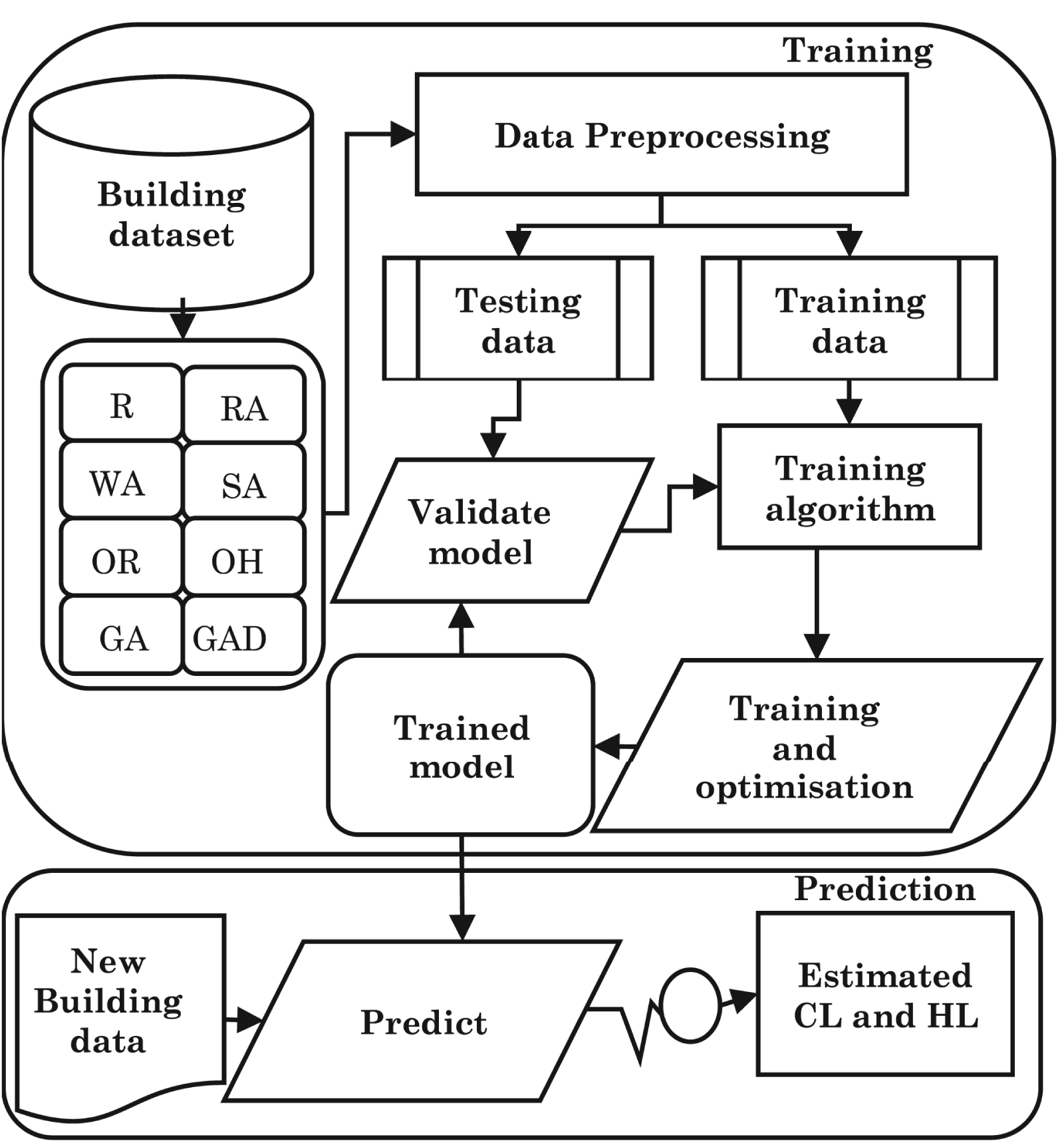
The proposed schematic diagram for modelling building energy.
In order to evaluate the performance of machine learning algorithms, two standard error-based and accuracy-based metrics were adopted: the Root Mean Square Error (RMSE) defined by Equation (1), which measures the deviation between predicted and actual values, and the coefficient of determination (R2) defined by Equation (2), which quantifies the proportion of variance in the dependent variable explained by the model. These complementary metrics allow a robust assessment of predictive performance across different modeling paradigms.


In which Yi is predicted value, Xi is observed value,
The selected machine learning algorithms were chosen to represent a diverse set of approaches commonly applied in building energy prediction (Al-Shargabi et al., 2022). The comparative models include linear models, which provide a simple and interpretable baseline; tree-based ensemble methods such as Random Forest and Gradient Boosting, which capture non-linear interactions and variable importance; kernel-based regressors such as Support Vector Regression, which are effective in modeling complex relationships in high-dimensional feature spaces; and neural networks, which can approximate highly non-linear patterns and are widely recognized for their strong predictive performance. By selecting models from these distinct families, we ensure a comprehensive comparative framework. This design not only enables an evaluation of predictive performance, but also highlights the trade-offs between accuracy, computational complexity, and interpretability when compared to the proposed fuzzy rule-based system.
K-Nearest Neighbors (K-NN) algorithm implements learning based on the nearest neighbors of each query point, where K is an integer value specified by the user. The K-NN algorithm deals with classification problems in a methodologically simple way: it predicts the class of a test sample by voting the classes of its K-nearest neighbors (where the neighborhood relationship is induced by a measure of the distance between the samples). When the K-NN model is used in the context of regression problems, voting is replaced by an aggregation (e.g., mean) of target values associated with nearest neighbors (Daulay et al., 2023).
Elastic net
Elastic net is a regularization technique for performing linear regression (Zou & Hastie, 2005). Assume a set of training data points S = {(xi; yi) / i = … N}, where xi is the input vector of p values and yi is the output value; and the approximation of regression function is assured by a linear model E(Y |X = xi) = β0 + xiT β. Elastic net solves the following problem:


Pα is a compromise between the lasso penalty in which α = 1 and the ridge regression penalty in which α = 0. In situations where there are many correlated predictor variables, or such as when p is much bigger N, elastic-net penalty is particularly useful.
Multiple linear regression, also referred to as multiple regression, is a statistical technique that forecasts the outcome of a dependent variable by combining many independent variables into a linear equation:

MLP is the most common feed forward artificial neural network (ANN) technique. MLP architecture consists of input layer, hidden layers, and output layer. Each layer contains a set of weighted neurons. MLP is trained using a variety of methods, including the BFGS Quasi-Newton (BFG), Back-Propagation (BP), Levenberg-Marquardt (LM), and Resilient Backpropagation (RP) (Perera et al., 2020). Mathematically, MLP with one hidden layer is represented in Equations (6) and (10):

The total of the inputs Xi is given by Equation (6), where α0j is the bias term of the hidden layer and αij is the weight vectors. In Equation (7), the output of the hidden layer Oj is given by using activation function f.

Equation (8) Specifies one of the most common activation functions, the sigmoid function.

Equation (9) specifies the total of the hidden layer's outputs (Oj), where β0k is the bias term of the output layer and βjk is the weight vectors.

The Results of the output layer (Yk) are provided by Equation (10),

Support Vector Machine (SVM) is proposed by VLADIMIR VAPNIK (Vapnik, 2013) who often used to solve regression problems and classification problems, it is characterized by its high precision which compete the precision of neural networks . Formally, Support Vector Machine uses S = {(xi; yi) / i = … N} a set of training data points, where xi is the input vector and yi is its output value. The algorithm uses a loss function called ε-insensitive defined by :

Figure 4 shows the SVM regression in a two-dimensional species, which is a linear regression defined using a loss function ε-insensitive. The model is defined as a minimization problem represented by Equation (9), taking into account the constraints defined in Equation (10). The support vector machine aims to reduce the complexity of the model by minimizing the value of



ε-insensitive loss in SVM regression.
The Random Forest algorithm creates a collection of decision trees that are combined to increase the accuracy of a prediction (Breiman, 2001). Random forest uses Bootstrap Aggregation thechnique during the training step, also referred to as Bagging. Bootstrap generates sample datasets for each model by randomly selecting rows and features from original dataset. After combining the outputs of all the models, the final decision is made based on a majority vote, this step is known as aggregation.
ExtraTrees Models
Extra-Trees method is an averaging algorithm based on randomized decision trees. This implies that by including randomness during their training, a diverse set of decision trees is produced. The prediction is given by averaging the results of the decicision trees (Geurts et al., 2006). When splitting a feature into child nodes, Extra-Trees chooses values at random and uses the entire dataset to reduce the bias of the model. However, the randomization of the feature value at which to split, increases the bias and variance.
Adaboost
AdaBoost can be adapted for regression problems as well. The basic idea is similar to classification, but instead of combining weak classifiers, it combines weak regressors to make a strong regressor. The weak regressors make predictions and the final prediction is made by a weighted average of the weak regressor predictions. The weights are updated after each iteration based on the errors made by the weak regressors, similar to the classification case. The algorithm continues until a specified number of weak regressors are combined, or the error rate is reduced to a desired level. The end result is a strong regressor that is more accurate than any individual weak regressor (Drucker, 1997).
The steps for AdaBoost algorithm for regression problems are: – Initialize the weights for the training examples: Assign equal weights to all training examples. – Train the first weak regressor: Train a simple regression model on the weighted training data. – Calculate errors: Calculate the prediction error of the weak regressor for each example in the training data. – Update weights: Increase the weight of examples that are misclassified by the weak regressor and decrease the weight of examples that are classified correctly. – Train the next weak regressor: Train another simple regression model on the updated weighted training data. – Repeat steps 3–5: Repeat steps 3–5 until either a specified number of weak regressors are combined or the error rate is reduced to a desired level. – Combine weak regressors: Combine the weak regressors into a single strong regressor by taking a weighted average of the predictions of each weak regressor. – Make predictions: Use the final strong regressor to make predictions for new data
XGBoost
XGBoost (eXtreme Gradient Boosting) is a powerful machine learning algorithm that is widely used for regression problems. It is an ensemble learning method that combines multiple decision trees to produce prediction. The XGBoost algorithm is known for its high accuracy and speed, making it one of the most popular algorithms for regression problems (Chen & Guestrin, 2016).
In XGBoost for regression problems, the algorithm starts with a single decision tree and uses the residuals (the differences between the actual values and the predicted values) to train additional decision trees. These trees are combined to create a final prediction. The algorithm also uses regularization techniques to reduce the impact of any one feature on the final prediction and prevent overfitting.
The steps involved in XGBoost for regression problems are: – Prepare the data: Clean and preprocess the data to remove any missing values or outliers. Split the data into training and testing sets. – Initialize the model: Start with a single decision tree, with a default set of hyperparameters. – Calculate the residuals: Calculate the residuals by subtracting the predicted values from the actual values for the training set. – Train the model: Use the residuals to train additional decision trees, which will be used to correct the predictions of the first tree. Repeat this process multiple times to create multiple decision trees. – Combine the trees: Combine the decision trees using a weighted sum, where the weight of each tree is proportional to its accuracy. – Regularize the model: Use L1 and L2 regularization techniques to reduce the impact of any one feature on the final prediction and prevent overfitting. – Make predictions: Use the combined decision trees to make predictions on the testing set. Evaluate the performance of the model using metrics such as mean squared error or mean absolute error. – Fine-tune the model: If the performance of the model is not satisfactory, fine-tune the hyperparameters and repeat the process. – Deploy the model: Once the model has been trained and fine-tuned, deploy it in a real-world application to make predictions.
The XGBoost algorithm is highly customizable, and the number of trees, the hyperparameters, and the feature selection process can be adjusted to improve the performance of the model.
Fuzzy Rules Based System Model
A fuzzy rule-based fuzzy (FRBS) is a method that uses fuzzy logic to map input data to output data. Due to the use of linguistic values to represent numeric data, the difference between a rule-based fuzzy system and other systems is interpretability. The architecture of fuzzy rule-based system contains four main components: Fuzzification interface, knowledge base, inference engine and defuzzification interface. The fuzzification interface is a set of mathematical operations that allows the system to assign an appropriate list of linguistic values to each input data. The inference engine is a reasoning method that uses the knowledge base to find the fuzzy set corresponding to the output by relying on the linguistic values determined by the fuzzification interface. The defuzzification interface converts the obtained fuzzy set into output data. The knowledge base consists of two bases: The Rulebase and the Database. The Rulebase is a set of fuzzy IF-THEN rules used by the inference engine in the reasoning process. For the database, it contains all parameters that allow the definition of linguistic variables and their linguistic values. There are two distinct approaches suggested in the literature to develop fuzzy rule-based systems: Linguistic fuzzy modeling and precise fuzzy modeling. Linguistic fuzzy modeling is used to develop MAMDANI fuzzy rule-based based systems (Mamdani, 1976) and precise fuzzy modeling is used to develop TAKAGI–SUGENO–KANG fuzzy rule-based based systems (Takagi & Sugeno, 1985). Figure 5 shows the MAMDANI FRBS approach; the fuzzy sets represent the consequents and the antecedents. The consequence is a weighted combination of input variables with fuzzy sets representing the antecedents of the TSK FRBS approach.

Linguistic FRBSs.
Two criteria are used for evaluating FRBSs, which are accuracy and interpretability. The accuracy is typically measured with the root mean square error. There are two types of interpretability (Mencar & Fanelli, 2008), (Ishibuchi & Nojima, 2007): The complexity and the semantics. Figure 6 illustrates the interpretability in DB and in RB. The complexity-based interpretability is designed to reduce the complexity of the obtained system, which normally is measured with the number of rules in RB, the number of antecedents per rule and the number of linguistic labels for each linguistic variable. On the other side, semantics-based interpretability is designed to preserve the semantics in KB, which normally imposes restrictions on the MFs in DB to preserve the meaning of the linguistic labels, these restrictions concern distinguishability, the coverage, the fuzzy ordering, the Normalization etc. In the RB, semantics-based interpretability requires certain constraints such as the consistency of rules, the number of rules fired simultaneously and the transparency of rule structure. Thus, for a good accuracy–interpretability balance in FRBSs, three requirements are necessary: The accuracy, the complexity, and the semantic interpretability.

Interpretability of linguistic FRBSs.
This section presents the structure and training process of the proposed Fuzzy Rule-Based System (FRBS), named FRLC (Fuzzy Rule Learning through Clustering). The current methodology builds upon our previously published works in (Bahani et al., 2018), (Bahani et al., 2020). Using embedded Database learning that encapsulates Rulebase learning, the architecture of the FRLC model is shown in Figure. 7, which comprises three main modules: Database learning, Rulebase learning, and Evaluation.
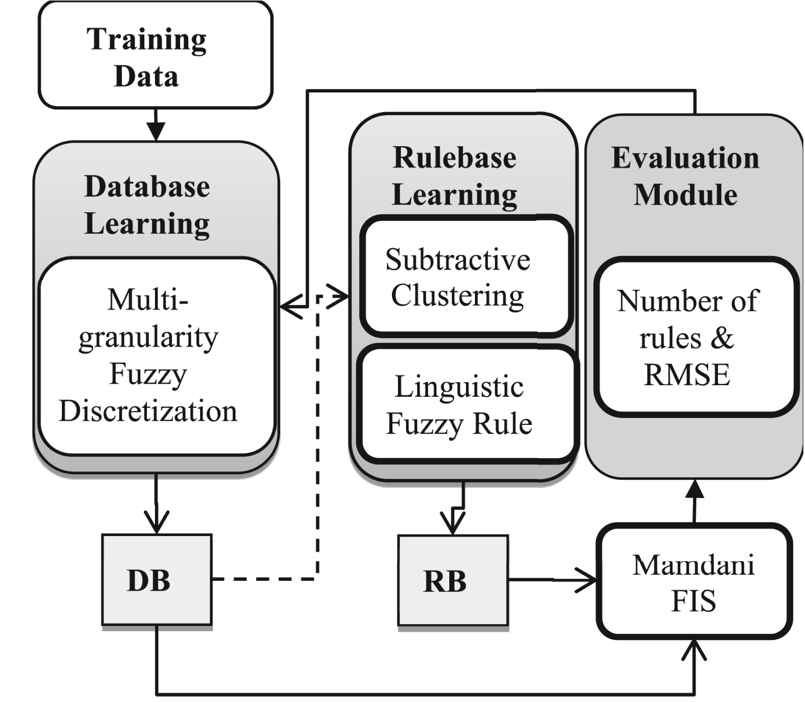
FRLC model.
The fuzzy database is constructed using a multi-granularity fuzzy discretization algorithm applied to a dataset consisting of multiple instances, each described by a set of input variables and one or more output variables. Each input variable is treated as a linguistic variable, with its universe of discourse discretized into a set of linguistic labels (e.g., Low, Medium, High), subject to interpretability constraints. The number of labels per variable is typically bounded within a predefined range, such as from 2 to 9 (de Oliveira, 1999). Each label is associated with a Gaussian membership function defined by a center and spread. The overall search space for label configurations is expressed as:
Rulebase Learning
After the fuzzy database is built, the next step is to generate a set of linguistic fuzzy rules that describe the relationship between the input variables and the output(s) of interest. This process, known as Rulebase Learning, is composed of two core stages: Subtractive Clustering, and Linguistic Rule Construction with Modifiers.
Subtractive Clustering Using Fuzzy Database Parameters
Fuzzy clusters are extracted using an adaptive subtractive clustering algorithm. The clustering process relies on a radius vector ra = (ra1,ra2,…,raM), where each component defines the influence zone of the corresponding input dimension. These radius values are derived from the Gaussian membership functions constructed during database learning. For each input variable, the fuzzy partition provides a set of membership functions characterized by their centers cjk and standard deviations σjk. The clustering radius raj for each variable is computed from the dispersion of these functions. The potential of each data point xi is calculated as:

Each extracted cluster is transformed into a linguistic fuzzy rule. This transformation includes two steps: linguistic Approximation: For each cluster center xiC, a linguistic label is assigned to each input variable by comparing its value to the centers of the membership functions using Euclidean distance:

Refinement with Linguistic Modifiers: Because the fuzzy partitions are uniform, some approximations may lack precision. To address this, linguistic modifiers such as Very (P = 2), Plus (P = 1.25), Minus (P = 0.75), More or Less (P = 0.5), Slightly (P = 1.7), and A Little (P = 1.3) are applied using Hamming distance to fine-tune the linguistic terms.
The fuzzy knowledge base is evaluated using a Mamdani-type fuzzy inference system (FIS), which uses the minimum t-norm for logical conjunctions and the Center of Gravity (COG) method for defuzzification. Model performance is assessed using two criteria: RMSE, to measure prediction accuracy, and number of fuzzy rules, to assess complexity. The evaluation is carried out iteratively: after each modification to the fuzzy database or rulebase, the model is re-evaluated using the selected metrics. Configurations that improve accuracy or reduce complexity are retained. This iterative evaluation loop continues until a satisfactory trade-off is achieved between performance and simplicity. The resulting fuzzy inference system is then considered finalized and ready for testing, validation, or deployment depending on the application context. To improve interpretability, don’t-care conditions are incorporated (Ishibuchi & Nojima, 2013), allowing rules to exclude variables that have little impact on the output. As a result, the final fuzzy rulebase includes rules with a variable number of antecedents depending on their relevance.
Results and Discussions
To assess the performance of FRLC in predicting cooling and heating loads, we used an energy efficiency dataset created by TSANAS and XIFARA (Tsanas & Xifara, 2012). Each data point (xi; yi) is represented by an output data vector yi representing the heating load and cooling load and an input data vector xi representing the building characteristics (See Figure. 3). TSANAS and XIFARA used the ECOTECT software to simulate twelve buildings of different shapes, leading to the generation of 768 data points (Al-Rakhami et al., 2019). The basic statistics are provided in Table 1. In our study, we first conducted an in-depth statistical analysis of the dataset to examine the impact of various building parameters on heating and cooling loads. The correlation analysis revealed that variables such as Overall height, Roof area, Surface area, Relative compactness, and Wall area exhibit significant relationships with the target variables (Table 2).
Basic Statistics of the Data Set.
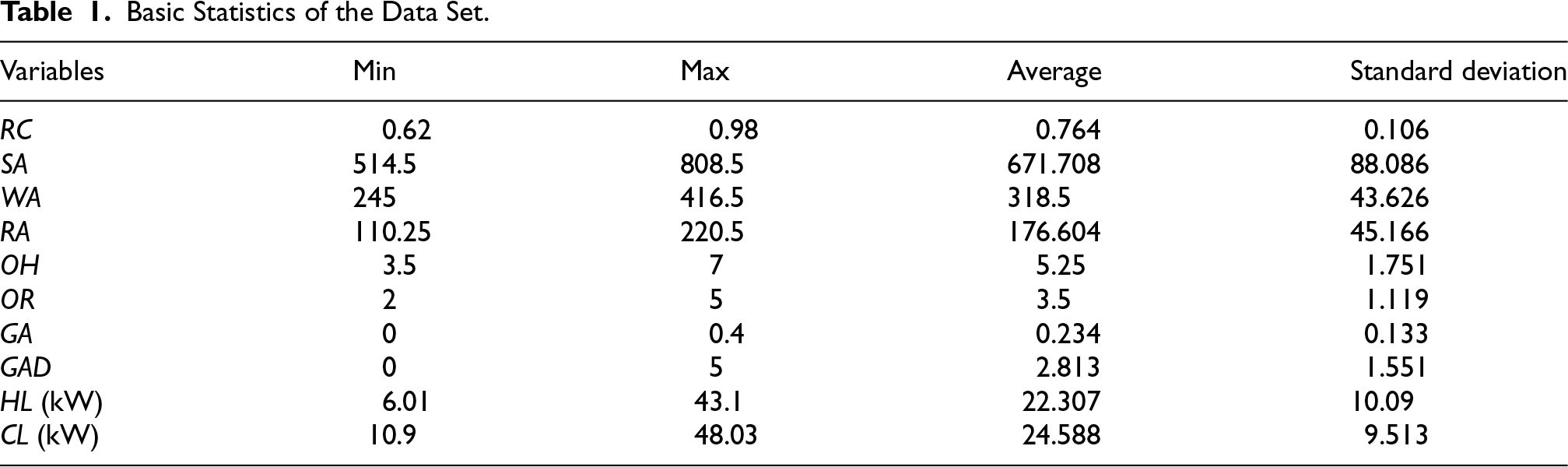
Basic Statistics of the Data Set.
Correlations with Heating Load and Cooling Load.

In contrast, Orientation showed no meaningful impact, as confirmed by ANOVA and Tukey's post-hoc tests (Kao & Green, 2008), (Tukey, 1949), leading to its exclusion from further analysis (Tables 3 to 5).
ANOVA Test:(Orientation).

Test de Tukey - Heating Load (Orientation): Multiple Comparison of Means - Tukey HSD, FWER=0.05.

Test de Tukey - Cooling Load (Orientation): Multiple Comparison of Means - Tukey HSD, FWER=0.05.

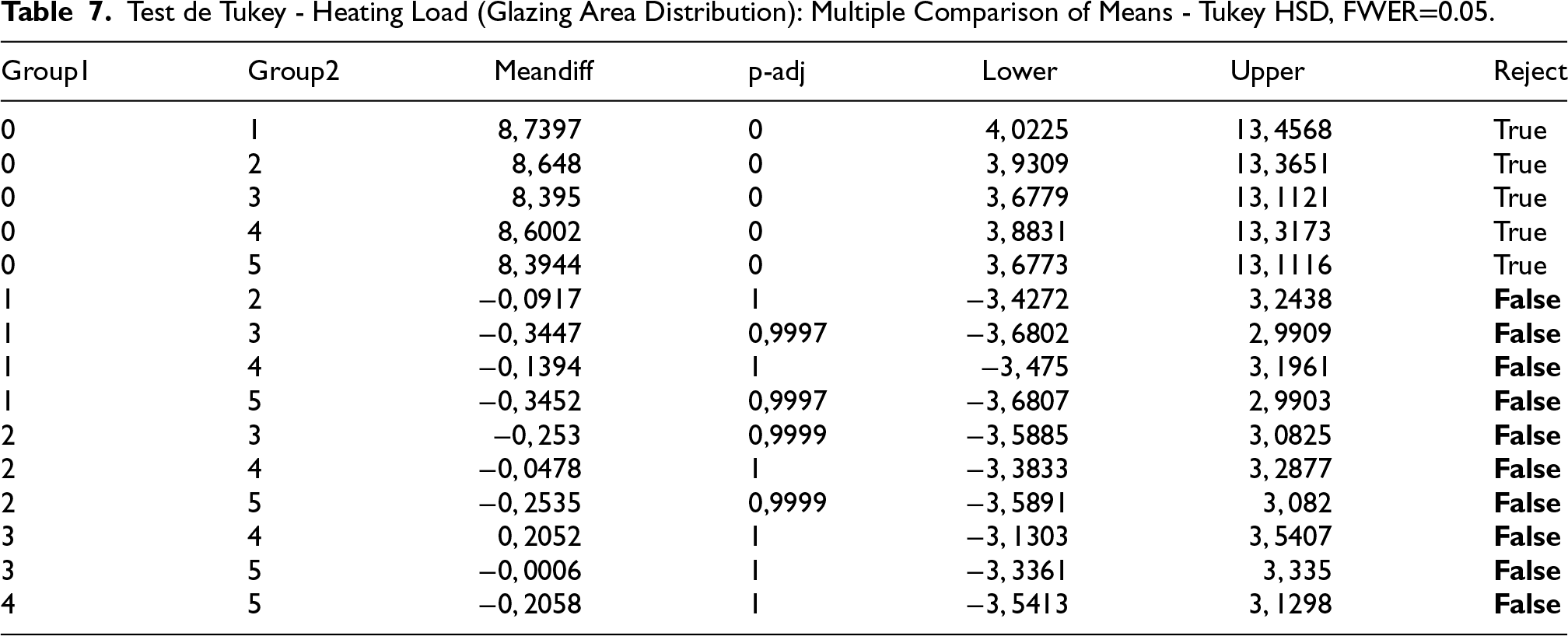
Furthermore, we investigated the Glazing area distribution variable and found that its values could be effectively grouped into two distinct categories due to the similarity observed between certain levels. This transformation not only simplifies the model but also enhances interpretability while preserving relevant information. The impact of this variable was further assessed using ANOVA and Tukey's tests, confirming its retained significance in predicting heating and cooling loads (Tables to 8). Following this preprocessing step, we proceeded to evaluate the performance of various machine learning models on the dataset, employing a 5-fold cross-validation approach.
ANOVA Test:(Glazing Area Distribution).

Test de Tukey - Heating Load (Glazing Area Distribution): Multiple Comparison of Means - Tukey HSD, FWER=0.05.
Test de Tukey - Cooling Load (Glazing Area Distribution): Multiple Comparison of Means - Tukey HSD, FWER=0.05.

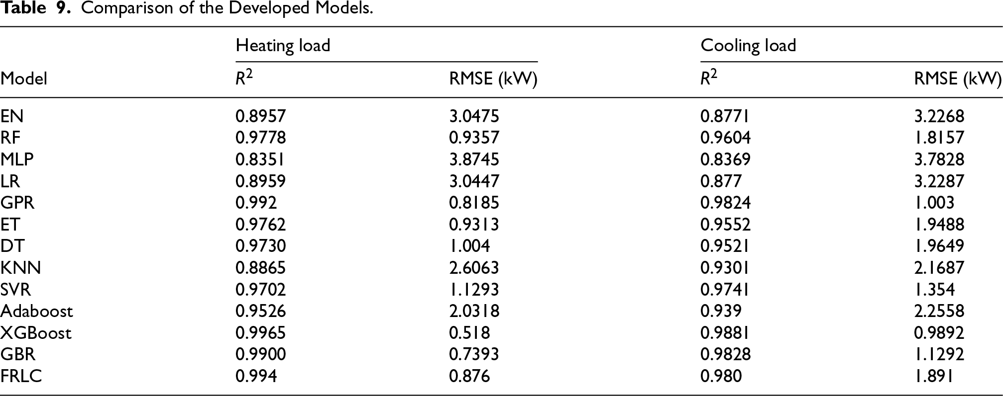
As presented in Table 9 and illustrated in Figure 8, the FRLC model is compared to 12 machine learning algorithms, with performance evaluated using the Root Mean Square Error (RMSE) and Coefficient of Determination (R2) for both heating load sand cooling load prediction. To ensure a robust and generalizable evaluation of all models, we adopted a 5-fold cross-validation approach. The dataset was randomly partitioned into five folds, with each fold serving once as the test set while the remaining folds were used for training and validation. Performance metrics (R2 and RMSE) were averaged across folds to ensure reliability.
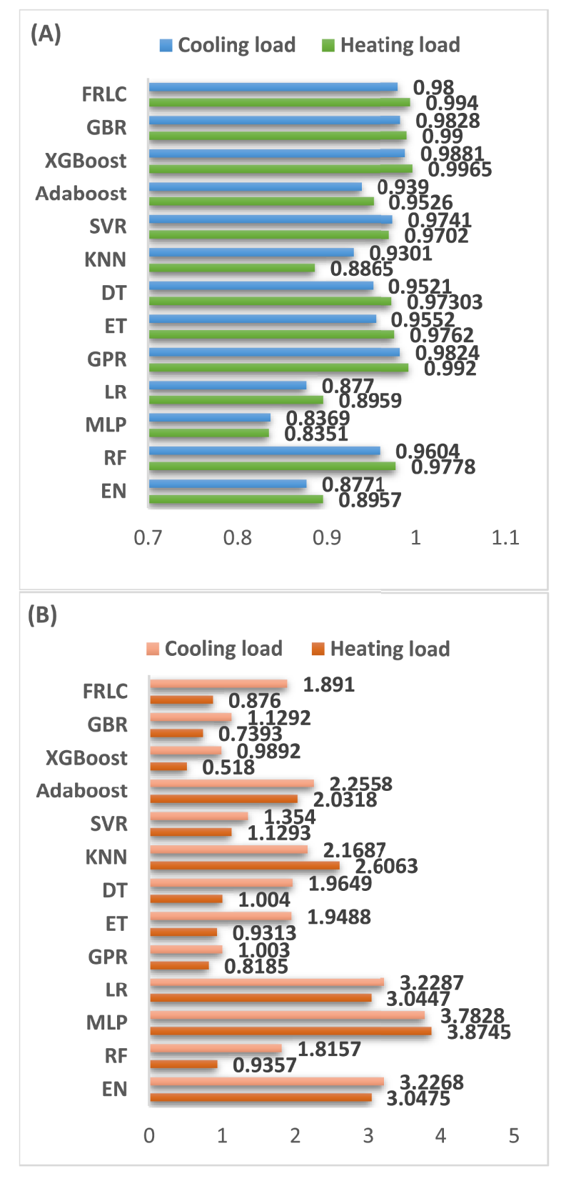
Performance of compared methods. (a) Based on R2 Measure, and (b) Based on RMSE Measure.
Comparison of the Developed Models.
For all machine learning models, we employed GridSearchCV from Scikit-learn to perform hyperparameter tuning. The optimization objective was to minimize RMSE on the validation folds, ensuring a fair and consistent comparison across all methods. Table 10 summarizes the optimal hyperparameter values selected for each model after cross-validation.
Optimal Hyperparameters Selected for Each Model Using GridSearchCV.

The FRLC model demonstrates strong performance in both tasks, achieving R2 scores of 0.994 for heating load and 0.980 for cooling load. These results position FRLC among the top-performing models, closely rivaling XGBoost, which remains the best model with 0.9965 for heating load and 0.9881 for cooling load. Other high-performing models include GPR (0.992 for heating, 0.9824 for cooling) and GBR (0.990 for heating, 0.9828 for cooling), both showing competitive predictive capabilities. On the other hand, models like MLP (0.8351 for heating, 0.8369 for cooling) and LR (0.8959 for heating, 0.877 for cooling) exhibit weaker performance, as indicated by their lower R2 scores.
In terms of RMSE, values range from 0.518 to 3.8745 for heating load and 0.9892 to 3.7828 for cooling load. The FRLC model achieves RMSE values of 0.876 for heating load and 1.891 for cooling load, maintaining its competitive edge. However, XGBoost outperforms all models by achieving the lowest RMSE values (0.518 for heating and 0.9892 for cooling), indicating its superior accuracy. Additionally, GPR (0.8185 for heating, 1.003 for cooling) and RF (0.9357 for heating, 1.8157 for cooling) also exhibit strong performance, closely matching FRLC. Conversely, models such as MLP (3.8745 for heating, 3.7828 for cooling) and LR (3.0447 for heating, 3.2287 for cooling) show significantly higher RMSE values, reflecting poorer predictive accuracy.
Overall, the FRLC model delivers excellent performance, standing out as one of the best-performing models in both heating and cooling load predictions. While XGBoost remains the top performer due to its slightly better accuracy, FRLC remains highly competitive, with results that place it among the leading models in terms of both R2 and RMSE.
One of the main challenges in traditional machine learning models is the trade-off between accuracy and explainability. Linear models such as Linear Regression and Elastic Net offer global interpretability through their coefficient-based structure, but their assumption of linearity limits their ability to capture complex relationships, resulting in lower predictive performance (R2 = 0.8959 for HL and 0.877 for CL). Decision trees, while providing some level of local explainability through explicit rules, become harder to interpret as depth increases (max_depth = 50 for DecisionTree), and ensemble methods like Random Forest and ExtraTrees further obscure the decision process by aggregating multiple trees. Although boosting algorithms (Adaboost, XGBoost, Gradient Boosting) achieve superior accuracy (XGBoost: R2 = 0.9965 for HL, 0.9881 for CL, RMSE = 0.518 for HL), they rely on hundreds of weak learners, making their predictions difficult to explain without external tools like SHAP or LIME. Similarly, kernel-based models (SVR) and neural networks (MLP) function as true black boxes, preventing direct interpretation of their decisions. In our study, MLP not only lacks explainability but also underperforms compared to other methods (R2 = 0.8351 for HL, RMSE = 3.87), questioning its relevance. These limitations highlight the need for a model that balances interpretability and predictive power, which our FRLC model effectively addresses.
Explainability of FRLC Model
Unlike traditional machine learning models, the FRLC model that we developed aims to reconcile interpretability and performance. This approach offers both global and local explainability through several key features: an interpretable rule-based Base,uniform discretization of linguistic variables, use of linguistic modifiers and a trade-off between accuracy and interpretability.
Global Explainability
The goal is to propose a predictive model that not only simulates reality but also explains the relationship between input and output data. Table 11 illustrates the number of membership functions and the corresponding linguistic labels for each linguistic variable. The GAD variables are represented by two linguistic labels, the GA variables by four linguistic labels, the RC and SA variables by eight linguistic labels, and the WA, RA, OH, HL, and CL variables each by nine linguistic labels.
Linguistic Variables and the Numbers of Their Linguistic Values.
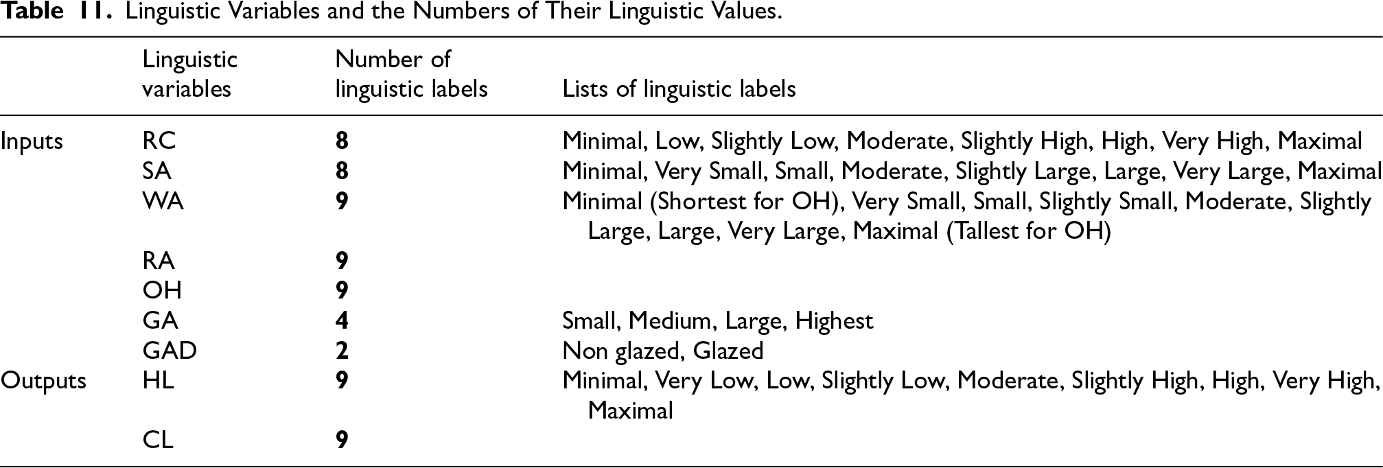
Linguistic Variables and the Numbers of Their Linguistic Values.
The system clearly explains the contribution of each variable as shown in Figure 9, the variables GAD, GA, RC, and WA were chosen to indicate the fuzzy partitions with 2, 3, 8 and 9 linguistic labels, respectively.

The fuzzy partitions of linguistic variables GAD (a), GA(b), RC(c), and WA(d).
The FRLC Rulebase consists of 37 rules, Table 12 presents the three firt rules of FRLC Rulebase, in which the linguistic modifiers are marked in bold and omitted conditions of a rule was described by “—” dashes. The linguistic formulation of the rules enables experts and engineers to analyze, refine, validate, or reject the results provided by FRLC, helping to mitigate the risk of incorrect assessments.
The First Three Rules from FRLC Rulebase.

A structural analysis of the 37 fuzzy rules reveals that many rules share similar linguistic patterns and differ only through secondary modifiers or slight variations in input configurations. This recurrence enables the entire rulebase to be organized into five coherent behavioral families, each representing a consistent thermal response pattern. These families preserve the transparency of the fuzzy model while enhancing its usability for early-stage architectural and engineering decision-making. – Roof-Dominant Family (13 rules) : a substantial number of rules assign high linguistic values to the roof area, particularly Very_Large and Maximal. These rules consistently indicate that buildings with large roof surfaces tend to exhibit moderate cooling loads, especially when the glazing ratio remains in the Small–Medium range. This highlights the influence of roof geometry on thermal demand even before material or insulation choices are considered. – Height-Driven Family (23 rules) : the overall height frequently appears in its extreme categories (Tallest or Shortest), demonstrating a strong dependence of thermal loads on vertical proportions. Configurations involving the Tallest category are typically associated with increased heating and cooling loads, emphasizing the need for enhanced envelope performance—such as optimized façade properties and insulation—in multi-storey building designs. – Glazing and Distribution Family (30 rules) : Glazing distribution appears in the vast majority of rules, most often in the Glazed modality, and interacts closely with the glazing ratio. This widespread presence reflects the significant impact of glazing-related parameters on cooling loads. Moderate glazing ratios combined with balanced distribution systematically reduce cooling peaks, whereas extreme or unbalanced glazing distributions contribute to higher heating loads. This family captures the central role of façade transparency in shaping thermal behavior. – Compactness and Wall Surface Family : a subset of rules associates higher compactness with reduced or linguistically modified wall area. These cases generally lead to more stable thermal performance, with moderate heating and cooling loads. This indicates that compact building shapes with lower wall exposure naturally mitigate thermal fluctuations, in line with principles of energy-efficient architectural design. – Linguistic Modifiers and Fine-Tuning Family : Many rules include linguistic modifiers such as slightly, more or less, minus, and very. While these modifiers do not alter the broader structural tendencies identified in the other families, they provide fine-grained adjustments that refine the thermal response. They enable smooth transitions between design alternatives—such as marginal changes in glazing, compactness, or height—thus giving the fuzzy model a nuanced capacity to support incremental design decisions.
Organizing the 37 fuzzy rules into these five behavioral families transforms the rulebase into a compact and actionable set of design guidelines. This distilled structure improves the interpretability and practical applicability of the fuzzy system, facilitating its integration into early-stage building design workflows while maintaining the full transparency of the underlying model.
Local Explainability
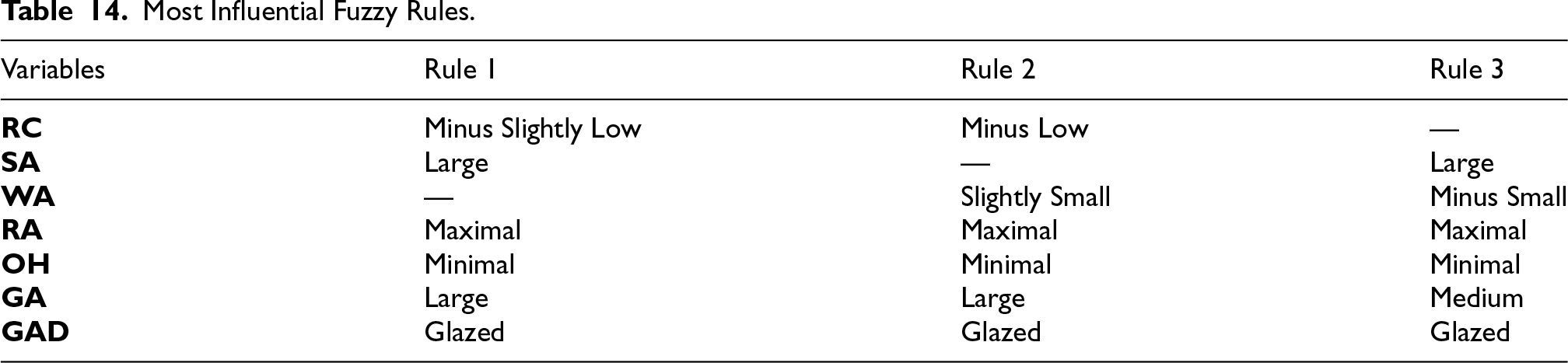
Local explainability aims to understand how specific building characteristics influence the prediction of heating load and cooling load. Thanks to the linguistic rule-based structure of our fuzzy system, each prediction is justified by a set of activated rules based on the input values. To illustrate the local explainability for Individual Predictions, we analyze a building with the following characteristics Table 13. FRLC model activates multiple rules, but only three main rules have the most significant impact on the prediction as showing in Table 14. Each rule contributes differently to the final prediction. The importance of the rules is weighted by their degree of activation (rule firing) Table 15.
Interpretation of Individual Predictions.

Interpretation of Individual Predictions.
Most Influential Fuzzy Rules.
Contribution of Each Rule and Variable Impact.

Rule 1 (RC = Slightly Low, SA = Large, RA = Maximal, GA = Large) has the strongest contribution to the prediction due to the highest activation degree (0.427). The slightly low RC and large SA slightly increase the thermal load, predicting HL = Slightly Very Low and CL = Very Low. Rule 2 (RC = Minus Low, WA = Slightly Small, RA = Maximal, GA = Large) has a moderate influence (activation degree of 0.243), where the effect of WA (Slightly Small) and RC (Minus Low) slightly reduces the thermal load, predicting HL = More or Less Very Low and CL = Very Low. Rule 3 (SA = Large, WA = Minus Small, RA = Maximal, GA = Medium) has the least influence (activation degree of 0.119), with the GA (Medium) and WA (Minus Small) effects slightly moderating the thermal load and adjusting the final prediction, predicting HL = Very Very Low and CL = Very Low. By combining these rules with their respective activation degrees, the system performs defuzzification to obtain the final numerical values: HL (Heating Load) = 12.003 kWh/m2 and CL (Cooling Load) = 16.373 kWh/m2.
This example demonstrates how FRLC model provides robust local explainability by identifying which building characteristics influence the prediction and how they do so. Relative Compactness, Surface Area, and Roof Area are the most influential variables in thermal load prediction, as they appear in all activated rules. Glazing Area and Wall Area have secondary effects, slightly adjusting the final prediction. The system clearly explains the contribution of each variable and provides complete transparency in the decision-making process, unlike black-box models such as neural networks. Thus, through this approach, heating and cooling load predictions become interpretable and justifiable, making the model highly suitable for expert decision-making.
To position our proposed FRLC model within the current landscape of explainable energy forecasting, this section compares its performance and interpretability against several recent studies that applied interpretable models to the Tsanas and Xifara dataset for predicting heating and cooling loads. Abdel-Jaber and Dirks (2024) employed decision trees and the RIPPER algorithm to construct rule-based classifiers, emphasizing native interpretability. Their approach enables stakeholders to follow decision paths directly, though performance metrics were only partially reported and the models remain relatively simple. Khastar et al. (2025) proposed a hybrid Radial Basis Function Neural Network (RBFNN) optimized through metaheuristics. Their method yielded excellent accuracy (R2 ≈ 0.99 for HL and 0.97 for CL), but interpretability was limited to post-hoc sensitivity analysis, with the underlying model remaining a black box. Salami et al. (2023) introduced an explainable tree-based ensemble model enhanced via Bayesian optimization and interpreted through SHAP values. This model demonstrated outstanding accuracy (R2 ≈ 0.9986 for HL and 0.9938 for CL), though the interpretability remains external, and computational overhead is higher.
Table 16 summarizes the key characteristics of each study in terms of model type, interpretability mechanism, and predictive performance. The FRLC model combines high accuracy with native, intrinsic interpretability. It uses a compact set of 37 fuzzy rules and requires only 8 input variables. With competitive results (R2 = 0.994 for HL, 0.980 for CL), the FRLC offers transparent and explainable forecasts, eliminating the need for post-hoc explanation tools and making it suitable for trustworthy deployment in real-world decision-making contexts.
Comparison of Recent Interpretable Models Using the Tsanas and Xifara Dataset.

Comparison of Recent Interpretable Models Using the Tsanas and Xifara Dataset.
The Tsanas & Xifara dataset used in this study is synthetically generated from DOE-2 simulation models and therefore does not include measurement noise, sensor irregularities, missing data, or operational anomalies typically found in real buildings. Because the data distribution is fully controlled, robustness tests (noise perturbation, missingness, distribution shift) and large-error sample analysis would not faithfully reflect real-world model behavior, as the dataset contains no natural uncertainty sources. For this reason, such analyses were not included in the present work. Future research will address robustness and error analysis on real monitored datasets, where variability, noise and extreme conditions are naturally present and more informative for evaluating model stability.
Conclusion
The building sector significantly contributes to economic growth but remains a major consumer of energy, requiring urgent optimization strategies. This study addresses the challenge of forecasting residential building energy consumption by developing an explainable fuzzy prediction model based on subtractive clustering and linguistic hedges. The proposed model balances interpretability and accuracy, offering a transparent decision-making process through linguistic fuzzy rules. Tested on a dataset of 768 residential buildings, the model utilizes eight input variables to predict heating and cooling loads. It is compared with Elastic Net, Random Forest, MLP, Linear Regression, Gaussian Process Regressor, ExtraTrees, Decision Tree, KNeighbors, SVR, Adaboost, XGBoost, and Gradient Boosting Regressor, demonstrating strong predictive performance while maintaining transparency. Unlike black-box models, our approach allows stakeholders to understand how building characteristics influence energy consumption, facilitating informed decision-making.The findings confirm that integrating XAI principles into energy forecasting enhances both trust and usability. Despite its promising results, the proposed approach still faces scalability and generalizability challenges that may constrain its robustness. Future research will address these issues by evaluating the FRLC model on larger and more diverse datasets, examining its adaptability across different building types and conditions, and refining both its hybridization strategies and knowledge base to improve accuracy while preserving interpretability.
Footnotes

Funding
The authors received no financial support for the research, authorship, and/or publication of this article.
Declaration of Conflicting Interests
The authors declared no potential conflicts of interest with respect to the research, authorship, and/or publication of this article.