Can the Learnability Criterion Ensure Determinacy in New Keynesian Models?

Abstract

Forward-looking rational expectation (RE) models such as the popular New Keynesian (NK) model do not provide a unique prediction about how the model economy behaves. We need some mechanism that ensures determinacy. McCallum (2012) says it is not needed because models are learnable only with the determinate solution and so the NK model, once learnt in this way, will be determinate. We agree the only learnable solution that has agents converge on the true NK model is the bubble-free one. But once they have converged, they must then understand the model and its full solution therefore including the bubble. Hence, the learnability criterion still fails to pick a unique RE solution in NK models.

JEL Classifications: C62, D84

Keywords

New Keynesian Taylor rule determinacy E-stability learnability

Introduction

Determinacy is a longstanding issue in rational expectations (RE) models with forward-looking terms (the first to focus on it were Gourieroux et al., 1982). These terms enable a ‘non-fundamental’ or a ‘bubble’ solution to be found besides the usual one only containing fundamentals. The usual practice is to ignore these alternative solutions. For example, in the New Keynesian (NK) Taylor rule model of inflation determination (which have been the centerpiece of monetary analysis over the past two decades), King (2000) and Woodford (2003) claim that bubble paths are somehow impossible.³ However, there needs to be a good reason to ignore these alternative solutions. As Cochrane (2011) has argued this is insufficient: (a) these paths are ‘possible’ (nothing would stop them if they happened) but (b) they are also incredible since they involve hyperinflation/hyperdeflation (‘the Fed blowing up the world’).

How much does all this matter? Models without determinacy (the absence of a unique RE solution) such as the popular NK model are problematic as they stand and so do not rate as models of interest. They do not provide a unique prediction about how the model economy—and thus the actual economy being modelled—behaves. So there must be some mechanism that ensures determinacy (the Taylor principle does not do it as argued by Cochrane, 2011). Consequently, a number of additional requirements have been proposed by various researchers in order to obtain a unique rational expectation equilibrium (REE).⁴

McCallum (2012) agrees with Cochrane’s analytical point on the non-uniqueness of REE but goes on to defend the NK model: the bubble paths are ‘not learnable’ and learnability is a condition for a model to be well founded. His thesis is that the bubble solution does not converge on the RE solution, that is, the bubble path is ‘not learnable’. However, the stable solution is learnable; hence, the NK model, when it is learnt, will have a unique stable solution. But it is hard to know what meaning to attach to the idea of a ‘solution’ (purely) being learnt.

In general, in the learning literature the related question asked is whether agents when learning will converge on the RE solution and so learn the RE model, so that henceforth it can operate as an RE model. Thus, the convergence is to the RE model. So does McCallum mean by ‘solutions are learnt’ (a) that people then know the model and it acts like an RE model, having thus been learnt? or does he mean (b) that people know the model and it is an RE model, but these people are only aware of one solution, that is, the stable one? If (a), then as we know they will know the general solution of an NK model which includes the bubble solution. If (b), then they have not learnt the model since they will be unaware of the general solution that it implies! In this case, after ‘learning’, we would have some model with an autoregressive expectation process, and not the NK—RE model. Thus, the latter would under (b) not be ‘supported’ by learnability.

Our article presents a new result—about learning as a way of closing down bubble solutions. It examines what McCallum could mean and how it bears on the determinacy issue. It also briefly surveys related articles. On what sort of bubbles our article deals with any bubble potentially affecting an RE solution. This bubble is thus part of the equilibrium in an RE model.

In the second section, we study determinacy in the standard three-equation NK model. We explain how researchers deal with multiple equilibria in these models. In the third section, we review the concept of E-stability, explain how this criterion is alleged to select the economically relevant RE solution in the cases in which multiple equilibria obtain and we show that it fails to do so. In the fourth section, we argue that a terminal condition on monetary behaviour justified by welfare can modify the NK model internally to make it determinate. The fifth section provides concluding remarks.

Eliminating Multiple Equilibria in New-Keynesian Models—The Role of the Taylor Principle

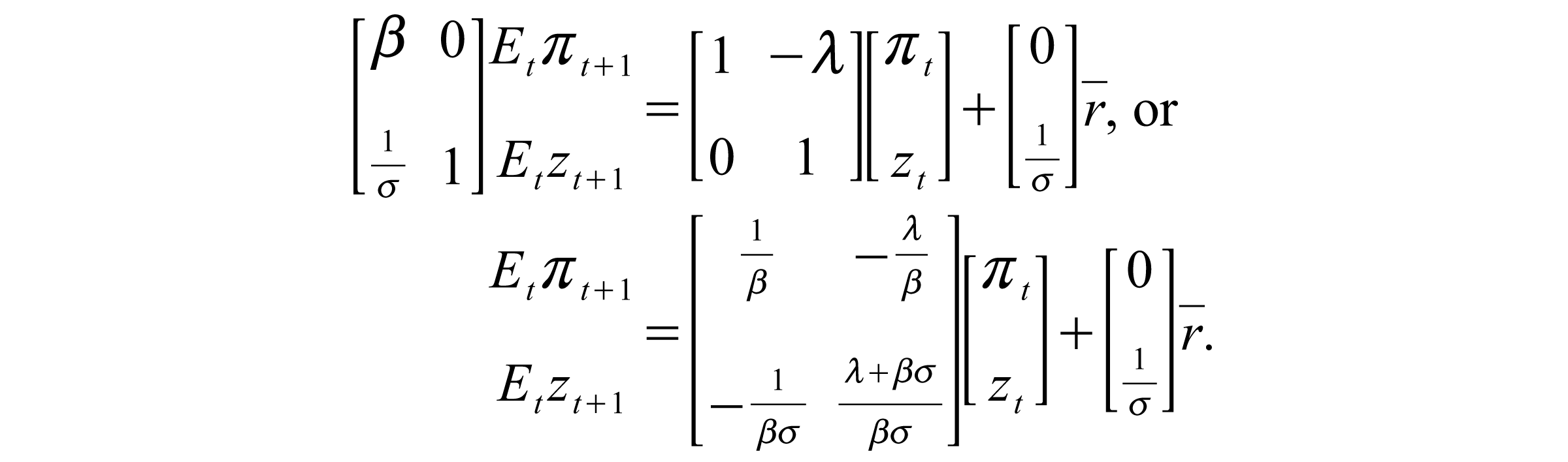
Now, let us consider a standard NK model with frictions (e.g., see Bullard and Mitra, 2002; Clarida et al., 1999; Woodford, 2003). For determinacy questions, we can work with a stripped-down model without constants or shocks:

_{t} E_{t}_{t 1} z_{t}, 0 1, > 0

(2.1)

z_{t} E_{t} z_{t 1} \frac{1}{} (r_{t} E_{t}_{t 1}), > 0

(2.2)

where π_t = denotes inflation, z_t = denotes the output gap and r_t = denotes the nominal interest rate. This representation can represent deviations from a specific equilibrium of a model with shocks (see Cochrane, 2011). The first equation is the NK Phillips Curve (NKPC). It is derived from the first-order conditions of intertemporally optimizing firms that set prices subject to costs.⁵ The second equation is a log-linear approximation to an Euler equation for the timing of aggregate expenditure, sometimes called an intertemporal investment–saving (IS) relation. This is the one that indicates how monetary policy affects aggregate expenditure: the expected short-term real rate of return determines the incentive for the intertemporal substitution between expenditure in periods t and t + 1.

As it stands, this is a two-equation, three unknown (π_t, z_t, r_t) model. The remaining equation required to close the system is a specification of monetary policy. We might, for example, close the model by assuming $r_{t} \overset{}{r}$ , a constant. Substituting for $r_{t} \overset{}{r}$ in (2.2), the model (2.1–2.2) can be written in the form,

\begin{matrix} [\begin{matrix} 0 \\ \frac{1}{} & 1 \end{matrix}] \begin{matrix} E_{t}_{t 1} \\ E_{t} z_{t 1} \end{matrix} [\begin{matrix} 1 \\ 0 & 1 \end{matrix}] [\begin{matrix} _{t} \\ z_{t} \end{matrix}] [\begin{matrix} 0 \\ \frac{1}{} \end{matrix}] \overset{}{r}, or \\ \begin{matrix} E_{t}_{t 1} \\ E_{t} z_{t 1} \end{matrix} [\begin{matrix} \frac{1}{} & \frac{}{} \\ \frac{1}{} & \frac{}{} \end{matrix}] [\begin{matrix} _{t} \\ z_{t} \end{matrix}] [\begin{matrix} 0 \\ \frac{1}{} \end{matrix}] \overset{}{r} . \end{matrix}

The stability/instability of the equilibrium is predicted solely on the make-up of the said Jacobian—J_E. Determinacy of the equilibrium requires that we have just enough stable roots as there are predetermined variables.

Proposition: If the number of eigenvalues of J_E outside the unit circle is equal to the number of non-predetermined variables (or forward-looking variables), then there exists a unique stable solution (Blanchard and Kahn, 1980).

Proposition: Let θ₁, θ₂ lie in the complex plane, then the θ_i’s (i = 1, 2) are both outside the unit circle if and only if the following conditions are satisfied:

\begin{matrix} |Tr (J_{E})| |1 Det (J_{E})| \\ |Det (J_{E})| > 1 . \end{matrix}

In the NK model set out above, both π_t and z_t are non-predetermined. Therefore, we need both of the eigenvalues of J_E:

J_{E} [\begin{matrix} \frac{1}{} & \frac{}{} \\ \frac{1}{} & \frac{}{} \end{matrix}],

to lie outside the unit circle. The eigenvalues of J_E, that is, θ₁ and θ₂, are computed by setting $\det (J_{E} I) 0$ . This gives a second-order polynomial in θ:

p ()^{2} Tr (J_{E}) Det (J_{E}),

where $Tr (J_{E}) () / () and Det (J_{E}) 1 /$ . For the usual parameter values in NK models $(0 1, > 0 and > 0)$ , the proposition $|Tr (J_{E})| |1 Det (J_{E})|$ is not satisfied.

Proposition: If the number of eigenvalues outside the unit circle is less than the number of non-predetermined variables, there is an infinity of stable solutions (Blanchard and Kahn, 1980).

The system does not provide a unique solution for π_t and z_t. For a fixed nominal interest rate ${(r}_{t} \overset{}{r})$ , the model economy will feature infinitely many non-explosive ouput and inflation paths—the ‘non-uniqueness’ problem (Taylor, 1977). That is, one could choose any value for π_t different from π*, and the solution describes a path that eventually takes the system back to the steady state (i.e., π_t → π*, as t → ∞). Because there is an uncountable number of such paths, each of which follows a path back to the steady state, it follows that there is a multiplicity of stable equilibria. In principle, any of these stable paths could be selected. The model does not restrict our choice.

The Taylor Principle and Determinacy of the Equilibrium

Suppose instead of a fixed interest rate rule we close our system (2.1–2.2) above by specifying a policy rule of the kind proposed by Taylor (1993) for the central bank’s operating target for the short-term nominal interest rate,

r_{t}_{}_{t},_{} > 1

(2.3)

Substituting this feedback rule (2.3) in (2.2) for r_t, the model (2.1–2.3) can be written in the form,

\begin{matrix} E_{t}_{t 1} \\ E_{t} z_{t 1} \end{matrix} [\begin{matrix} \frac{1}{} & \frac{}{} \\ \frac{_{} 1}{} & \frac{}{} \end{matrix}] [\begin{matrix} _{t} \\ z_{t} \end{matrix}] .

As before, the eigenvalues of J_E, that is, θ₁ and θ₂, are computed by setting $\det (J_{E} I) 0$ . This gives a second-order polynomial in θ:

p ()^{2} Tr (J_{E}) Det (J_{E}),

where $Tr (J_{E}) () / ()$ and $Det (J_{E}) (_{}) / ()$ . For a unique stable solution, we need both of the eigenvalues of J_E to lie outside the unit circle. Clearly, proposition 2 is satisfied provided $_{} > 1$ .

The crucial question is how does the Fed plan to stabilize inflation in this model? In this model, $E_{t} z_{t i}$ and $E_{t}_{t i}$ explode in any equilibrium other than z = 0, π = 0. According to Bullard and Mitra (2002) and other NK modellers, $_{} > 1$ (the Taylor principle) would stabilize inflation. But how does it rule out the unstable path? According to Bullard and Mitra (2002), the intuition for this result is that any deviation of the private-sector-expected inflation from the RE value leads to an increase in the real interest rate when the Taylor principle is satisfied. This reduces the output gap through Equation (2.2), which in turn reduces inflation through Equation (2.1). Such a policy, therefore, succeeds in guiding the initially non-rational private sector expectations towards the RE value.⁶

Unfortunately as Cochrane (2009, 2011) has pointed out, the standard NK model logic works differently. The Taylor principle destabilizes the economy. If inflation rises, the Fed commits to raising future inflation, and leads us into a nominal explosion. That is, if the current inflation misbehaves the Fed threatens to implement such paths (hyperinflation or hyperdeflation). Thus, the threat is to ‘blow up the world’—and this threat is supposed to be so terrifying that private agents expect the stable path instead. No economic consideration rules out the explosive solutions.⁷

This example makes it crystal clear that inflation determination comes from a threat to increase future inflation if current inflation gets too high. If inflation takes off along a bubble path, what is there to stop it in this model? The NK answer is: just the dreadful thought that this might happen. This is because in this model, the monetary authority is absolutely committed to raising interest rates more than one for one with inflation, for all values of inflation. For only one value of inflation today, will we fail to see inflation that explodes. NK modellers thus conclude that inflation today jumps to this unique value.

But how do they rule out the explosive equilibria? Here, NK authors become vague, saying that such paths would be ‘inconceivable’ and hence ‘ruled out by private agents’.⁸ The problem as pointed out by Minford and Srinivasan (2011a, b) is twofold: first, these threats are not credible. The reason is that once inflation or deflation happens, carrying through on the threat is a disastrous policy. As a result, self-destructive threats are less likely to be carried out ex-post, and thus less likely to be believed ex-ante. The second problem with these threats is that even if they were credible and did actually happen, there seems to be nothing to stop people following the implied paths. Clearly, they will prefer the stable path; but how can they be sure it will happen, given that all the paths are feasible. While undesirable from a social viewpoint, they do not appear to be impossible. Hence, there is nothing to make them infeasible. McCallum (2009a, 2012) agrees about the existence of this problem and proposes to rule these paths out by the ‘learnability criterion’ to which we now turn our attention.

Ruling Out Unstable Equilibria in New-Keynesian Models—The Learnability Criterion

In this section, we review the concept of E-stability (learnability) and explain how McCallum (2012) used this criterion for the selection of the economically relevant RE solution in cases in which the unstable (or bubble) path obtains. Recall the NK model we developed earlier:

_{t} E_{t}_{t 1} z_{t}, 0 1, > 0

(3.1)

z_{t} E_{t} z_{t 1} \frac{1}{} (r_{t} r_{t}^{n} E_{t}_{t 1}), > 0

(3.2)

where following Bullard and Mitra (2002) we have replaced r_t with $r_{t} r_{t}^{n}$ , where r_t is the nominal interest rate and $r_{t}^{n}$ is the natural rate of interest, assumed to obey:

r_{t}^{n} r_{t 1}^{n}_{t}, 0 1 .

As this model has two equations but three unknowns (π_t, z_t, r_t), we need a further equation for the nominal interest rate to close the model. As before, consider a contemporaneous version of the Taylor rule:⁹

r_{t}_{}_{t},_{} > 1 .

(3.3)

Substituting (3.3) into the expectation IS equation and using the NKPC, we can write the system as

x_{t} {BE}_{t} x_{t 1} r_{t}^{n},

(3.4)

where $x_{t} [_{t}, z_{t}]$ and

B \frac{1}{_{}} [\begin{matrix} 1_{} \end{matrix}],

where the form of γ is omitted since it is not needed in what follows. Since both π_t and z_t in the system are free, we need both of the eigenvalues of B to be inside the unit circle for determinacy. As we have already seen, this is satisfied for the model in the question provided, $_{} > 1$ .¹⁰ But how does the Fed plan to stabilize inflation in this model? As we have seen $E_{t} z_{t i}$ and $E_{t}_{t i}$ explode in any equilibrium other than z = 0, π = 0. How to rule out such explosive equilibria?

E-Stability and Learnability

Let us recast agents in our model as econometricians and ask whether, if endowed with the correct reduced form model for x_t, these agents could learn the parameterization of this model (β, σ, λ, Φ_π, ρ) which we assume is unknown to them. That is, we assume that the agents have the correct perceived law of motion (PLM) and posit that by running regressions each period, as new data become available, they might learn the model parameters, that is, they would learn to have REs. So the central question is: if agents estimate a statistical model which is a correct specification of an REE, under what circumstances will the estimates converge to that REE?

We now define precisely the concept of E-stability. For the study of learning, we endow agents in our model with a PLM of the form,

x_{t} a {cr}_{t}^{n}

(3.5)

which corresponds to the unique stablesolution (also the minimum state variable (MSV) solution in McCallum’s terminology). Here, a and c are the undetermined coefficients. This more general form allows for a constant term for this model.

Learning agents would use the PLM to form expectations of $x_{t 1}$ :

E_{t} x_{t 1} a c r_{t}^{n} .

Substituting the learning agent’s forecast into Equation (3.4), we obtain the actual law of motion (ALM) implied by the PLM,

x_{t} B (a c r_{t}^{n}) r_{t}^{n} Ba (Bc) r_{t}^{n}

(3.6)

Using (3.5) and (3.6), we can define a map, T, from the PLM to the ALM as

T () (\begin{matrix} Ba \\ Bc \end{matrix}),

where $[a, c]$ . Expectational stability (E-stability) is determined by the following matrix differential equation:

\frac{d}{d} T ()

(3.7)

where τ denotes artificial or notional time. The fixed points of Equation (3.7) give us the MSV solution. We say that a particular MSV solution $(\overset{}{a}, \overset{}{c})$ is E-stable (learnable) if the fixed point of the differential Equation (3.7) is locally asymptotically stable at that point. The conditions for E-stability of the MSV solution $(\overset{}{a}, \overset{}{c})$ are given in Proposition 10.3 of Evans and Honkapohja (2001a). Component by component, we have

\begin{matrix} \frac{da}{d} (B 1) a \\ \frac{dc}{d} (B 1) c . \end{matrix}

Using the results of Evans and Honkapohja (2001a), we need the real parts of the eigenvalues of $D (T (\overset{}{}) \overset{}{})$ to be less than zero, that is, the eigenvalues of both B and Bρ to have real parts less than one for E-stability. The eigenvalues of Bρ are given by the product of the eigenvalues of B and ρ, and since 0 < ρ < 1, it suffices to have only the eigenvalues of B to have real parts less than one for E-stability. As shown above, the characteristic polynomial of B is given by

p ()^{2} Tr (B) Det (B),

where Tr(B) = (βσ + λ + σ)/(σ + Φ_πλ) and Det(B) = (σβ)/ (σ + Φ_πλ).

Both eigenvalues of B are inside the unit circle if and only if both of the following conditions hold (see Bullard and Mitra, 2002)

|Det (B)| 1

(3.8)

|Tr (B)| |1 Det (B)|

(3.9)

Condition (3.8) implies the inequality $_{} > (1)$ , which is trivially satisfied since $0 1$ . Condition (3.9) is satisfied provided $_{} > 1$ . Recall that the Taylor principle was also a necessary condition for the determinacy of the REE. It turns out that the condition that ensures that the MSV solution is E-stable (learnable) is identical to the condition that guarantees uniqueness of REE, that is, the Taylor principle.

The Learnability Criterion for Selection of the Economically Relevant RE Solution

McCallum in a series of articles (2003, 2004, 2007, 2009a, b, 2012) has proposed E-stability and learnability criterion for the selection of the economically relevant RE solution in the cases in which the unstable, or bubble, path obtains. He has also suggested that this condition acts generally in RE models as the support for ruling out bubble paths and getting the MSV solution. His main point is that the bubble solution does not converge on the RE solution, that is, the bubble path is ‘not learnable’. However, the stable solution is learnable; hence, the NK model, when it is learnt, will have a unique stable solution.

This point can be briefly reviewed. For clarity, we shall concentrate on a frictionless NK model used by both Cochrane (2009) and McCallum (2012). This model has the advantage of transparency and so the least risk of confusion for the general argument.¹¹ In this model, our semi-reduced form solution is

0 b_{1} [(1_{1})_{t} e_{t} E_{t}_{t 1}],

where the monetary policy error, $e_{t} e_{t 1}_{t}$ with ε_t being white noise and with $|| 1$ ), and μ₁ > 0 is the Taylor principle.

This model has a bubble-free or MSV solution (1) $_{t} \frac{1}{1_{1}} e_{t}$ . It also has a bubble solution (2) $_{t} \frac{1}{1_{1}} e_{t} B_{t}$ , where B_t is a sunspot which is expected to explode at the rate $(1_{1})$ , so that $E_{t}_{t 1} \frac{}{1_{1}} e_{t} (1_{1}) B_{t}$ ; or equivalently $_{t} \frac{1}{} e_{t} (1_{1})_{t 1}$ . Notice that the general solution of the model is (2). That is to say, (2) expresses in one expression ‘what the model implies’ about the path(s) of inflation, the endogenous variable. (1) is only a solution if B_t is ignored: but according to the model it cannot be. McCallum’s point is that, while solution (1) above is E-stable, solution (2) is not. He goes on to say that as a consequence, solution (2) cannot occur in practice (because if a solution cannot be learnt, then it has no way of coming into being)—and thus that solution (1) is in fact the only outcome that can be predicted by the model.

To see this point, it is convenient to express our model in the form (3.4) above. Thus, we have

_{t} {BE}_{t}_{t 1} e_{t},

(3.4.1)

where $B 1 / 1_{1}$ and $(1 / 1_{1})$ . Is the bubble solution learnable? Suppose we endow agents in our model with a PLM of the form,

_{t} {ae}_{t} c_{t 1},

(3.5.1)

which does not correspond to the MSV or fundamental solution (solution (1) above). Recall that the agents assume that data are being generated by the process $_{t} {ae}_{t} c_{t 1}$ , but that they do not know the parameters a and c. At time t, they have estimates (a_t, c_t) which they use to make their forecasts, so that $E_{t}_{t 1}$ is given by

E_{t}_{t 1} a (c) e_{t} c^{2}_{t 1} .

Substituting the learning agent’s forecast into Equation (3.4.1), we obtain the ALM implied by the PLM,

_{t} [Ba (c)] e_{t} {Bc}^{2}_{t 1}

(3.6.1)

Using (3.5.1) and (3.6.1), we can define a map, T, from the PLM to the ALM as

T () (\begin{matrix} Ba (c) \\ {Bc}^{2} \end{matrix}),

where $[a, c]$ . E-stability is determined by the following matrix differential equation $\frac{d}{d} T ()$ . Component by component, we have

\begin{matrix} \frac{da}{d} (B (c) 1) a \\ \frac{dc}{d} (Bc 1) c . \end{matrix}

Using the results of Evans and Honkapohja (2001a), we need the real parts of the eigenvalues of $D (T (\overset{}{}) \overset{}{})$ to be less than zero, that is, the eigenvalues of both B(ρ + c) and Bc must have real parts less than one for E-stability. Notice that the stability condition is satisfied if agents use the bubble-free or stable solution (c = 0). In this case, it suffices to have only the eigenvalues of Bρ to have real parts less than one for E-stability. Since 0 < ρ < 1, it suffices to have only the eigenvalues of $B (1 / 1_{1})$ to have real parts less than one for E-stability which is satisfied provided, μ₁ > 0.

By contrast, if agents in our model are endowed with a PLM of the form, $_{t} {ae}_{t} c_{t 1}$ , where $_{t 1}$ is an extraneous state variable which is expected to explode at the rate $c 1_{1}$ , then convergence to (3.5.1) occurs with probability zero. Notice in this case that the eigenvalues of both $B (c) (1_{1} / (1_{1})) > 1$ and Bc = 1 do not satisfy the stability requirement. This example makes it clear that if agents do least-squares learning (as in Evans and Honkapohja, 2001a) assuming any of the solution expressions that are not bubble-free, they will not converge on the NK–RE model. What is the intuition behind this result? The reason the PLM for the ‘unique stable’ solution is learnable is because, as a ‘backward-looking solution’ it is stable in the usual way (all eigenvalues inside the unit circle), whereas the ‘unstable’ PLM (for the rogue solutions) is simply unstable backwards and so presumably cannot be learnt because it fluctuates wildly, forming no patterns in the data that converge on a unique steady equilibrium path. Thus, agents would give up on the unstable formula, realizing they were not learning. We can see no reason in broad terms to question this conclusion.

In sum, there are two possible outcomes for a learning model in this situation where agents’ learning of the expectations converges on the REE.

Assumption (a): the learning agents discover the reduced form, viz. the stable solution for the expectations variable and the solutions for the other variables. Then, knowing the structural form of the RE model and assuming the model is identified, they can work back to the structural parameters and thereby ‘learn the RE model’.¹² This outcome—where agents end up learning the full RE model, so that the model becomes an RE model after learning—seems to be what many understand is meant when in the learning literature it is (frequently) said that ‘learning converges on Rational Expectations’.¹³ Notice that it requires knowledge of the structural form (identification is also needed but this is a general requirement for any RE model to be of interest and so we can assume it is met for any model being discussed). Those authors who set up models of learning of this type in effect are assuming that the learning is of specific elements in the structural model, but not of the model’s form; in other words they know they are dealing with an RE model and they know its equations, such as an NKPC, a Taylor rule and an IS curve. In fact, in McCallum (2012), the knowledge of the structural form is implicitly assumed when agents in his model pick a reduced form to learn.¹⁴ Without this knowledge, they would find the right reduced form by a long process of search; they would have to search not only over reduced form parameters but also over the form itself—which variables to include, with what lags, etc.

The fundamental problem with McCallum’s thesis under assumption (a) is that while the only learnable solution that has agents converge on the true NK model is the bubble-free one; once they have converged, they must then understand the model and its full solution which includes the bubble. What have these agents in the NK model learnt? They have learnt the structural parameters of the model including the Fed’s reaction function, that is, a response coefficient on inflation greater than one. They have also learnt that in this model if inflation takes off along a bubble path there is nothing to stop it! Agents have learnt that in the NK world with the Taylor rule, the monetary authority is absolutely committed to raising interest rates more than one for one with inflation, for all values of inflation. If inflation rises, the Fed commits to raise future inflation and leads us into a nominal explosion. Therefore, the bubble solution is a legitimate solution in this model. Like Adam and Eve after eating the apple, they will then know too much and will be tormented by the general solution. Thus, the learnability criterion cannot stop these agents in the NK model, once convergence has occurred and it has thereby been learnt, from reverting to the true general solution. Hence, the learnability criterion still fails to pick a unique RE solution in NK models.

Assumption (b): while the agents discover the reduced form as above, they do not have the knowledge of the structural form. In this case, they cannot work back to the structural parameters since they do not know what structural parameters there are in the model. In this case, the RE model exists and is solved with expectations that are ad hoc but nevertheless it coincides with the stable solution of the model. In our example, agents take expectations of the inflation solution they have discovered; they are rational in the sense that they are using the correct solution and take mathematical expectations of it. However, notice that this is not an RE model in the usual sense that agents know the model and solve it; instead, they have ‘learned expectations’ that coincide with the (stable) model solution. In practical terms, this means that the model is vulnerable to Lucas’ critique: if the exogenous processes change, the expectation variable solution will change and agents will have to learn the new one. Policymakers will need to allow for this in policy optimization: thus, this ‘learning model’ will in time converge to the new solution. But this behaviour is different from that of a ‘full RE’ model where, as policy changes, agents at once adjust their behaviour and expectations to the new policy rule.

This, (b), is a useful clarification of McCallum’s position. It reveals that learnability can indeed lead to a ‘learned RE model’ in which expectations coincide with the stable solution. Thus, an RE model with two solutions, one unstable and the other the unique stable one, will under learning converge on the unique stable one. This model, if agents are incapable of learning the true RE model because they do not know its structural form, will be the final outcome. Thus, under (b) learnability does rule out the bubble paths but at the cost of creating an RE model, that is, ‘learned RE’ rather than ‘full RE’; the NK model, for example, can be considered as having only the unique stable solution but only on the understanding that this has come about through learning and if the exogenous processes change this solution will need to be re-learnt.

What Mechanism Inside the Model Can Remove Indeterminacy in NK Models?

Here, we refer to two articles that we recently wrote (Minford and Srinivasan, 2011a, b) which McCallum (2012) cited: these argue that we can rule out bubbles by providing an internal mechanism to the model. Our idea is similar to that of Obstfeld and Rogoff (1983) and see Cochrane (2011) for a comprehensive survey of other somewhat similar approaches. Also, one can see in a loose way that the European Central Bank’s (ECB) second (money) pillar could be interpreted as a mechanism of this sort.

The idea is to use transversality conditions for nominal variables analogous to those for real variables; we posit money demand and money supply functions. The latter mimics the Taylor rule in ‘normal times’ (i.e., money is supplied to meet the Taylor rule interest rate setting). However, if a bubble path for inflation were to occur, then the money supply would revert to a ‘fixed-inflation’ rule—similar to a ‘fixed exchange rate’ rule—in which money supply would be whatever was needed to enforce the constancy of inflation. This terminal condition acts to terminate any bubble prospectively; hence, no bubble path can occur and the normal Taylor rule is always observed.

This also deals with indeterminacy when there is no unique stable path, the ‘non-uniqueness’ problem—an example is the Taylor rule before the 1980s according to Clarida et al. (2000) when they argued that the Taylor principle did not hold $(_{} 1)$ . The terminal condition also disables these bubble paths (though here these are implosive or stable, the variance of inflation is still unbounded).

Conclusion

Models without determinacy are problematic as they stand and so do not rate as models of interest. On this, we can all agree, including McCallum and Cochrane. So there must be some mechanism that ensures determinacy. McCallum says it is not needed because models are learnable only with the determinate solution and so the NK model, once learnt in this way, will be determinate. We agree that the only learnable solution that has agents converge on the true NK model is the bubble-free one. But once they have converged, under normal assumptions (that the model is identified and they know the structural form) they will then understand the model and its full solution, therefore including the bubble. Hence, the learnability condition still fails to select the determinate solution. So the problem remains. If instead we assume that, because, for example, they do not know the structural form, they cannot go beyond the learned solution to understand the model, then they remain stuck in a ‘learned RE’ model, rather than the usual full RE–NK model; such a model would require the solution to be re-learnt every time the exogenous processes change. Hence, under this assumption, learnability does not underpin the NK model of the usual sort. Terminal conditions on monetary behaviour justified by welfare can, however, provide the necessary mechanism, converting NK models into proper NK models that can be used by economists in the usual way.

Footnotes

Acknowledgements

We thank an anonymous referee for helpful comments and suggestions.

Notes

References

Blanchard

Kahn

C.M.

(1980). The solution of linear difference models under rational expectations. Econometrica, 48(5), 1305–1313.

Bullard

James

Mitra

Kaushik

(2002). Learning about monetary policy rules. Journal of Monetary Economics, 49(6), 1105–1129.

Calvo

G.A.

(1983). Staggered prices in a utility-maximizing framework. Journal of Monetary Economics, 12(3), 383–398.

Clarida

Gali

Gertler

(1999). The science of monetary policy: A new keynesian perspective. Journal of Economic Literature, 37(4), 1661–1707.

Clarida

Gali

Gertler

. (2000). Monetary policy rules and macroeconomic stability: Evidence and some theory. The Quarterly Journal of Economics, CXV(1), 147–180.

Cochrane

J.H.

(2009). Can learnability save new-Keynesian models? Journal of Monetary Economics, 56(8), 1109–1113.

Cochrane

J.H.

. (2011). Determinacy and identification with Taylor rules. Journal of Political Economy, 119(3), 565–615.

Evans

G.W.

Honkapohja

(2001a). Learning and expectations in macroeconomics, frontiers of economic research. Princeton, NJ: Princeton University Press.

Evans

G.W.

Honkapohja

. (2001b). Economics of expectations, international encyclopedia of the social and behavioral sciences. Elsevier Science, 8, 5060–5067.

10.

Evans

G.W.

Honkapohja

. (2008). Learning in macroeconomics. New Palgrave Dictionary of Economics (2nd ed.).

11.

Friedman

B.M.

(2003). The LM curve: A not-so-fond farewell. NBER working paper 10123.

12.

Gourieroux

Laffont

Monfort

(1982). Rational expectations in dynamic linear models: Analysis of the solutions. Econometrica, 50(2), 409–425.

13.

King

R.G.

(2000). The new IS-LM model: Language, logic, and limits. Federal Reserve Bank of Richmond Economic Quarterly, 86(3), 45–103.

14.

McCallum

B.T.

(2003). Multiple-solution indeterminacies in monetary policy analysis. Journal of Monetary Economics, 50(4), 1153–1175.

15.

McCallum

B.T.

(2004). Consistent expectations, rational expectations, multiple-solution indeterminacies, and least-squares learnability. In Minford

Patrick

(Ed.), Money matters: Essays in honour of Alan Walters (pp. 11–34), Cheltenham, UK: Edward Elgar Publishing.

16.

McCallum

B.T.

. (2007). E-stability vis-à-vis determinacy results for a broad class of linear rational expectations models. Journal of Economic Dynamics and Control, 31, 1376–1391.

17.

McCallum

B.T.

. (2009a). Inflation determination with Taylor rules: Is new Keynesian analysis critically flawed? Journal of Monetary Economics, 56(8), 1101–1108.

18.

McCallum

B.T.

. (2009b). Rejoinder to cochrane. Journal of Monetary Economics, 56(8), 1114–1115.

19.

McCallum

B.T.

. (2012, July). Issues concerning determinacy, learnability, plausibility, and the role of money in new Keynesian models. NBER working paper no. 18215.

20.

Minford

Patrick

Srinivasan

Naveen

(2011a). Determinacy in new Keynesian models: A role for money after all? International Finance, 14(2), 211–229.

21.

Minford

Patrick

Srinivasan

Naveen

. (2011b). Ruling out unstable equilibria in new Keynesian models. Economics Letters, 112(3), 247–249.

22.

Obstfeld

Rogoff

(1983). Speculative hyperinflations in maximizing models: Can we rule them out? Journal of Political Economy, 91(4), 675–687.

23.

Taylor

J.B.

(1977). Conditions for unique solutions to macroeconomic models with rational expectations. Econometrica, Econometric Society, 45(6), 1377–1385.

24.

Taylor

J.B.

. (1993). Discretion versus policy rules in practice. Carnegie-Rochester Conference Series on Public Policy, 39(1), 195–214.

25.

Taylor

J.B.

(Ed.) (1999). Monetary policy rules. Chicago: University of Chicago.

26.

Woodford

(2003). Interest and prices: Foundations for a theory of monetary policy. Princeton, New Jersey: Princeton University Press.