Global Financial Crisis,Capital Inflows and Policy Trilemma: An Analysis of the Indian Experience

Abstract

In the context of the global financial crisis, this article analyzes the behaviour of capital inflows in India during the period from 1993.2 to 2012.4. It also examines the question, how have the policy makers in India dealt with the ‘policy trilemma’ in a regime of liberalized capital inflows? The study finds that the volatility of capital inflows increased after the global financial crisis. Further, due to the global financial crisis, there were substantial changes in the relative importance of the factors that explain capital inflows. Although the ‘pull factors’ played major roles in both the periods, before and after the crisis, there were significant changes in their relative importance. In the first sub-period, real effective exchange rate and foreign exchange reserves played the most important roles in determining the capital inflows whereas in the second sub-period, it was only current account balance. While dealing with ‘policy trilemma’, we observed that the monetary policy independence was maintained in the period before the crisis which was sacrificed in the later period.

JEL Classification: F30, F32, F39

Keywords

Policy trilemma global financial crisis capital inflow India

Introduction

The global financial market is currently in an unprecedented turmoil caused by the 2007 global financial crisis. The Indian financial markets, more liberalized and open since 1991, have experienced some vulnerability as a fall out of the global shocks. Capital inflows in India since economic reforms of 1991 have resulted in certain benefits in the form of greater liquidity and larger foreign exchange reserves. However, portfolio capital inflows came with considerable risks presenting challenges for policy makers, as has been reflected in the then Chief Economic Advisor Raghuram Rajan’s caution against over-dependence on portfolio capital inflows, which brought hot money. His advice, instead, was to focus more on the foreign direct investment (The Hindu, 2012). The reason is that the portfolio capital inflows tend to be highly volatile and thus potentially destabilizing as witnessed by the recent disruptions of financial markets. There was the reversal of capital flows in India since the beginning of 2007 till the end of 2011. Several researchers have argued that the ‘Quantitative Easing Programme’ of the United States, which led to unconventional monetary expansion through large-scale asset purchases, was primarily responsible for the reversal of capital flows in the aftermath of the global financial crisis. For the monetary authorities, arresting reversal of capital flows is surely a difficult task to handle. Tumbling stock prices, soaring foreign exchange rates and credit crunch are only a few urgent issues to be addressed in this regard. As the volatility of capital inflows in India has increased in the aftermath of the global financial crisis, it has been raising a number of concerns. To the extent that the volatility is driven by the fickleness of international investors, it creates a risk of financial instability.

India appears to have employed a mix of policy measures to prevent this financial instability. In response to the increased volatility of capital inflows after the global financial crisis, policy makers introduced some macroprudential measures to keep up the growth of the productive sectors. The Reserve Bank of India responded by facilitating monetary expansion through several instruments such as the Cash Reserve Ratio (CRR) (which was reduced to 5 per cent in July 2009 from 9 per cent in August 2008) and Statutory Liquidity Ratio (SLR) stipulation and open market operations including the Market Stabilization Scheme and Liquidity Adjustment Facility (LAF). Further the repo rate was reduced from 9 per cent in October 2008 to 4.25 per cent in July 2009 and the reverse repo rate was reduced to 3.25 per cent in July 2009 from 6 per cent in October 2008 to increase the flow of credit to the productive sectors.

In order to draw any realistic policy implications of recent experience of volatility in capital flows in India, it is essential to understand the exact characteristics and determinants of the capital flows. The literature on capital flows categorizes the factors influencing cross-country capital flows into two groups. The first group is composed of the so-called ‘push factors’. Push factors refer to the external determinants such as interest rates, economic growth and all economic activities and regulations related to the cross-border transactions in financial assets between countries. The second group includes the ‘pull factors’, which refer to the domestic determinants in a particular country such as domestic interest rates, growth rate, inflation, macroeconomic stability, current and capital account balances, stock market development and trade volume.

Determining the relative importance of these two types of factors driving capital inflows becomes crucial when the policy makers attempt to control capital inflows in the capital recipient countries. If the push factors are dominant in affecting capital inflows, the policy makers have little room to manage capital flows. In contrast, in case capital inflows are mostly affected by the pull factors, domestic policy makers will have greater control on the capital inflows exercised through measures that influence cross-border capital transactions.

In designing the domestic policy, the policy makers in an open economy are confronted with the new challenges to deal with ‘policy trilemma’. The trilemma refers to the difficulty of simultaneously targeting the exchange rate, pursuing an independent monetary policy and having a full financial integration. The basic premise of the policy trilemma is that a trade-off exists between monetary policy independence, exchange rate stability and financial integration and that changing one component is necessarily associated with a corresponding change in a combination of the other two components. The theoretical basis for this approach is the seminal Mundell-Fleming framework, which shows that with free capital mobility monetary policy is ineffective under fixed exchange rates, while it is fully effective under flexible rates (Fleming, 1962; Mundell, 1963). Some recent studies have extended the Mundell-Fleming framework further, to consider the managed floating exchange rate system (Bofinger & Wollmershauser, 2003; Bofinger, Mayer & Wollmershauser, 2006). As India has followed this system since 1993, we find it useful to draw insights from these studies. These studies develop a theoretical framework for a managed floating exchange rate system, in which the central bank targets an unannounced exchange rate path together with a short-term interest rate. In order to guarantee the simultaneous and independent use of the interest rate and the exchange rate as operating targets, the central bank has to control the exchange rate by sterilized intervention in the foreign exchange market. Setting two operating targets is based on the assumption that the two targets are subject to an internal and an external equilibrium condition. According to the external equilibrium, the exchange rate path and the interest rate are set in line with the uncovered interest parity condition, while according to the internal equilibrium, two operating targets under the managed floating could be reached by attaining a monetary condition index (MCI) which is based on the combination of the real interest rate and the real exchange rate. Optimum MCI is achieved by the central bank when it minimizes an inter-temporal loss function. Therefore, in this framework, the uncovered parity condition and the monetary condition index play a crucial role. It is to be noted that the studies by Bofinger and Wollmershauser (2003) and Bofinger, Mayer and Wollmershauser (2006) consider perfect mobility of capital. As India operates under imperfect mobility of capital, managed float with sterilized intervention cannot be followed in the long run. However, in the context of these discussions, it is imperative to examine how the policy makers have dealt with the policy trilemma in a regime of liberalized capital inflows in India.

A related issue in this context is the uncovered interest parity condition. According to the uncovered interest parity condition, capital inflows depend on the differential between the domestic interest rate and the world interest rate and also on the depreciation of exchange rates. Hence, uncovered interest parity condition is an important element of the trilemma and it is important to examine if there is a one-to-one relationship between changes in exchange rates and interest differentials.

This article addresses a set of questions in the context of global financial crisis relating to the liberalized regime of capital inflows in India since 1991. We specifically address the following questions: Was there any structural break in the capital inflows in India? How volatile was the capital inflow in India? Did the volatility increase after the global financial crisis of 2007? What are the main drivers of the capital inflows in India? Has there been a sea-change in their behaviour before and after the global financial crisis? How was the policy trilemma addressed while managing capital flows? Was the uncovered interest parity condition maintained?

This article makes an attempt to answer these questions on the basis of the quarterly data for India for the period from 1993.2 to 2012.4. The second section provides an overview of capital inflows in India. The third section addresses the first two questions, namely, whether the nature of capital inflows in India was volatile and whether the volatility has increased due to global financial crisis. The fourth section presents an analytical framework relating capital inflows and policy trilemma. The fifth section reports the empirical results. We conclude in the sixth section.

An Overview of Capital Inflows in India

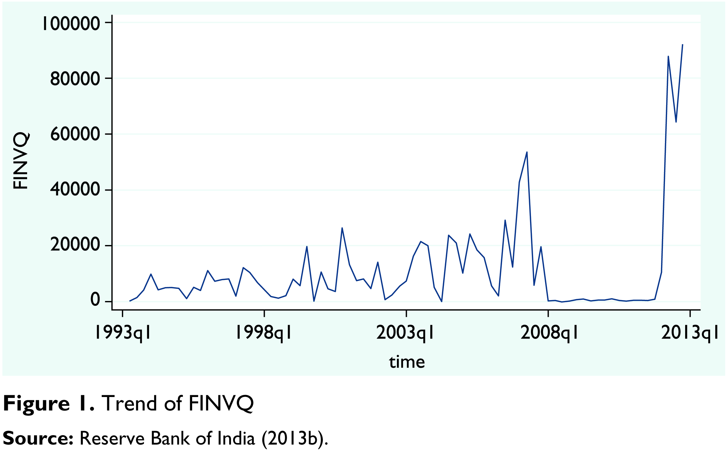
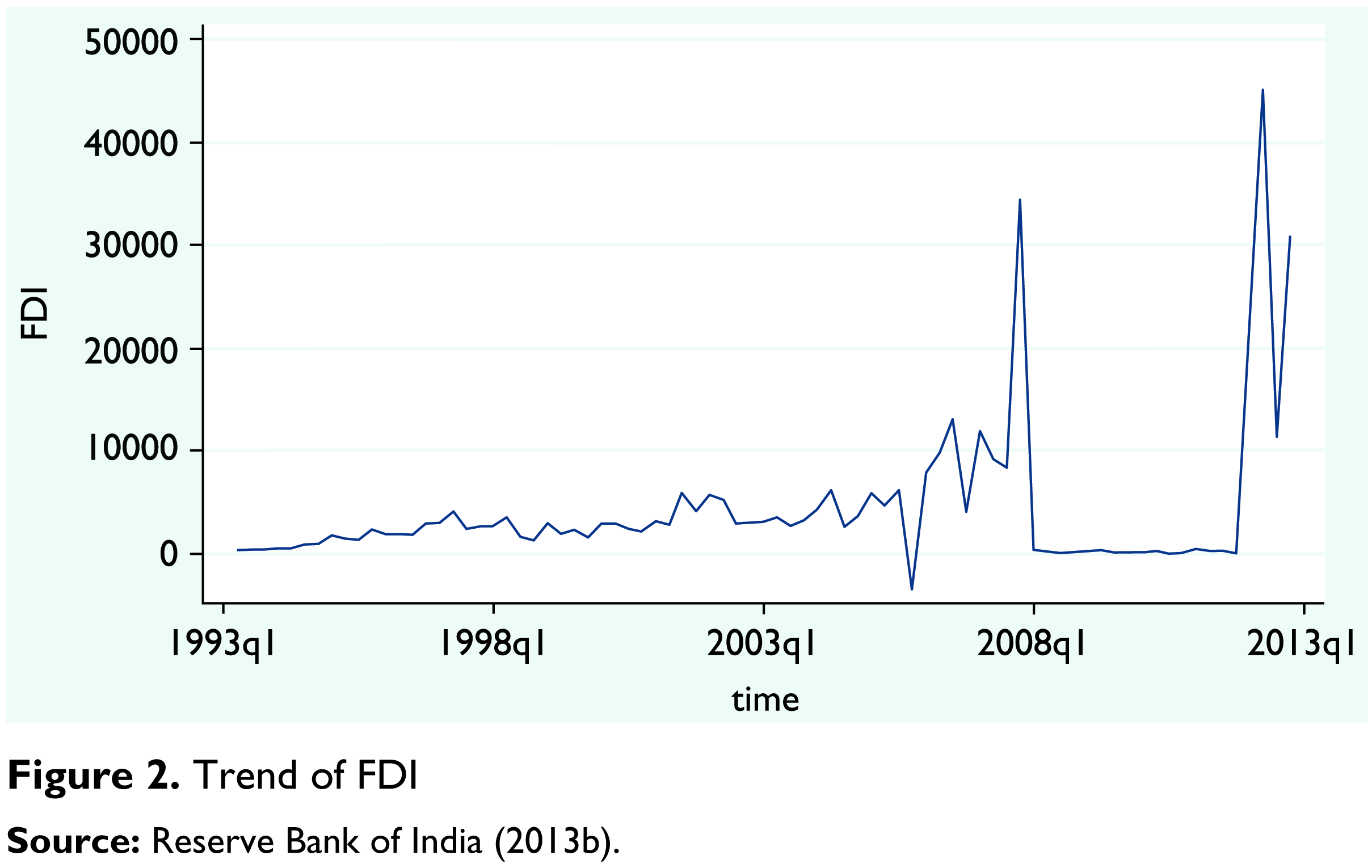
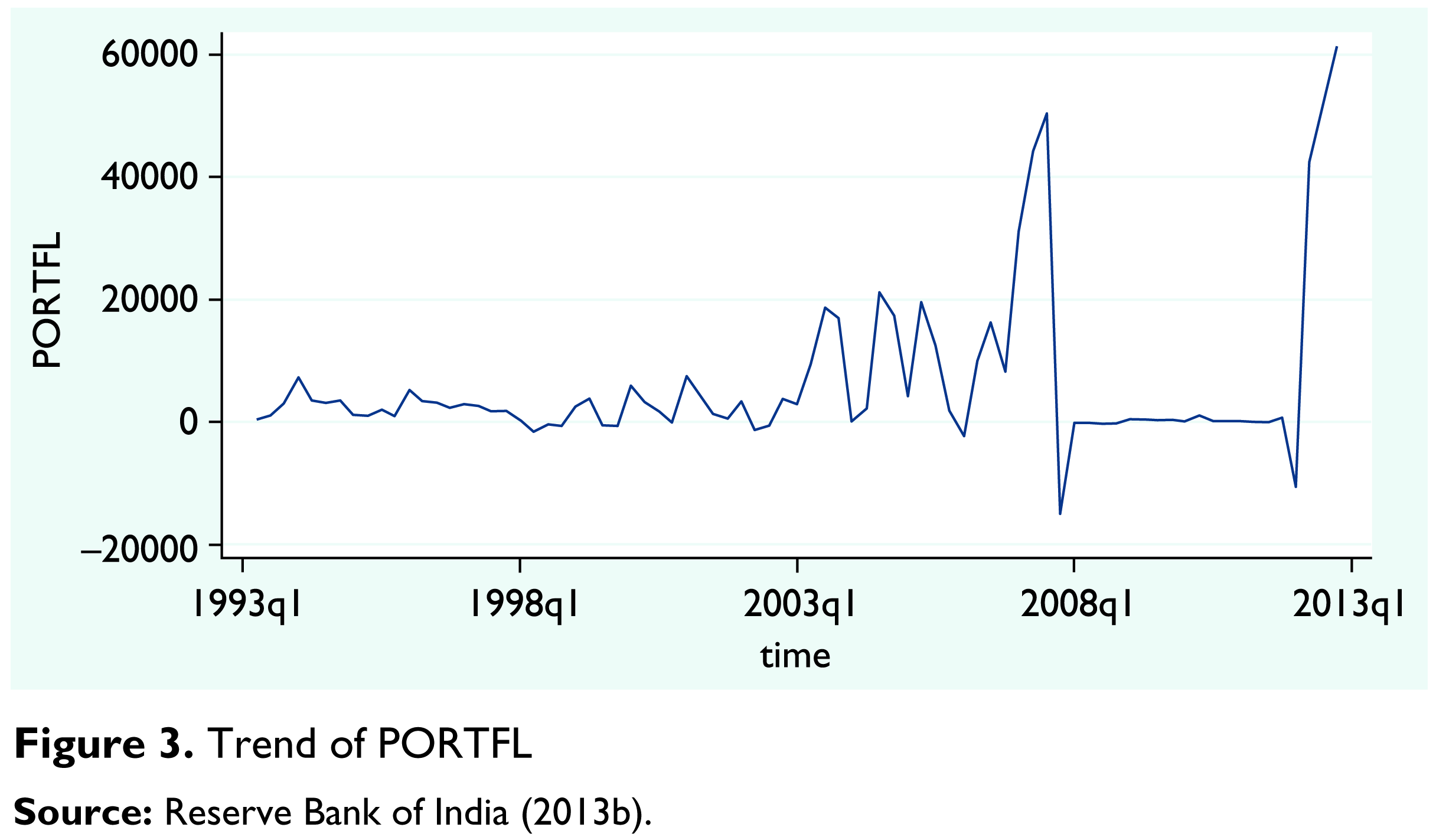
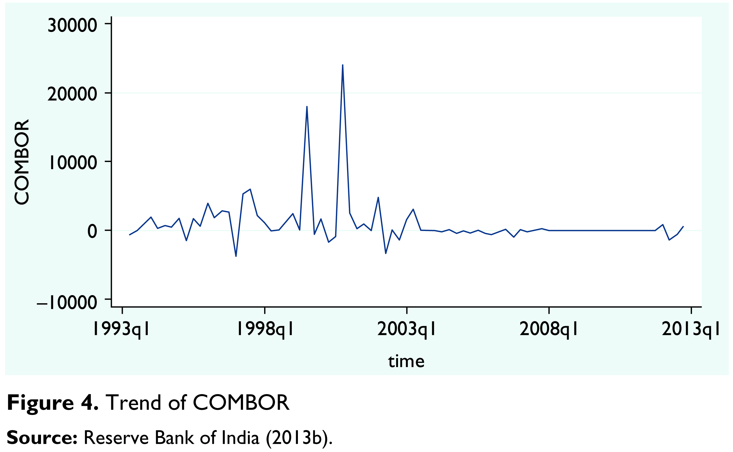
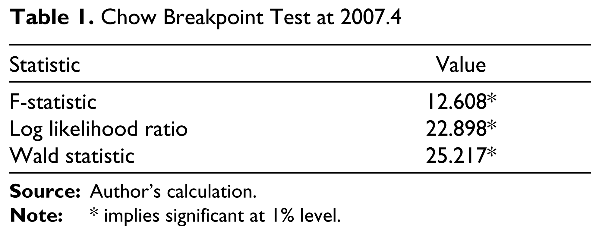
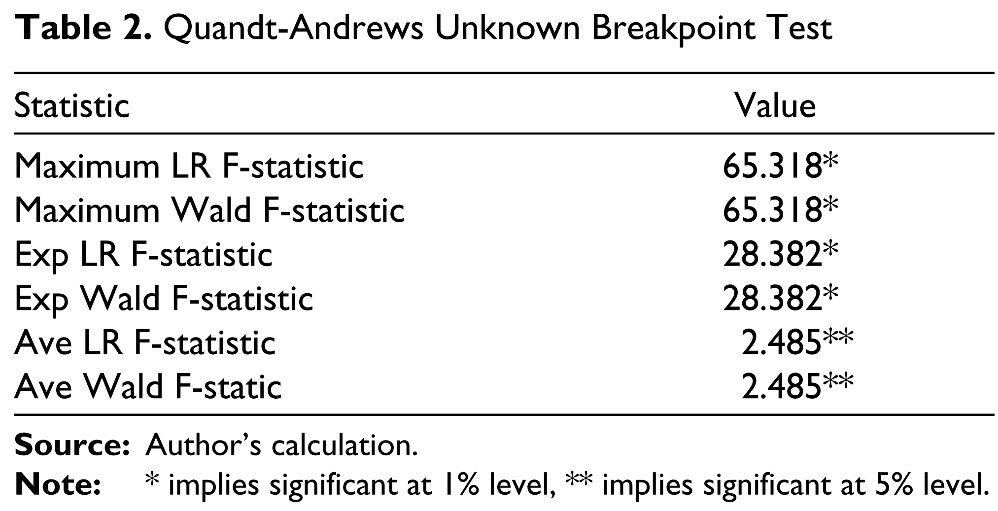
In this article, net inflow of capital (FINVQ) is taken to be the sum total of net foreign direct investment (FDI), net portfolio investment (PORTFL) and net external commercial borrowing (COMBOR). In Figure 1, we report the trend of FINVQ from 1993.2 to 2012.4. It appears that in spite of moderate fluctuations, net inflow of capital showed an increasing trend till 2007.4. Then due to the global financial crisis, there was a reversal of capital flow and the declining trend in net capital inflow continued till 2011.4. The rising trend resumed again in the first quarter of 2012. The trend of FDI is reported in Figure 2. It is evident that FDI exhibited an upward trend till 2007.4 and then it declined sharply and remained at that level till 2011.4 and resumed the upward trend again since 2012.1. Similar picture emerged from the trend of PORTFL as reported in Figure 3. Figure 4 presents the trend of COMBOR. In terms of volume, the inflow due to external commercial borrowing appears to be quite low and the trend is almost steady till 2003.2 except in the two quarters, namely, the third quarter of 1999 and the fourth quarter of 2000. Since 2003.2, the trend of COMBOR declined sharply. To examine if there was a structural break in the trend of FINVQ, we have applied two tests, namely, Chow breakpoint test and Quandt-Andrew unknown breakpoint test. The difference between these two tests is that in the former, we specify the breakpoint in the null hypothesis and whereas in the latter, our null hypothesis is that, there are no breakpoints within 5 per cent trimmed data. A different level of trimmed data could also be chosen. Tables 1 and 2 report the results of these two tests, respectively. From Table 1, we observe that all the three test statistics, F-statistic, Log likelihood ratio and Wald statistic, are significant at 1 per cent level which suggests that we accept the alternative hypothesis that there was a structural break at 2007.4. On the other hand, from Table 2 we observe that the first four test statistics are significant at 1 per cent level and the remaining two test statistics are significant at 5 per cent level, which indicate that the alternative hypothesis of existence of breakpoints within 5 per cent trimmed data is accepted. Hence, the Quandt-Andrews test confirms that there were some structural breaks in the trend of FINVQ and the Chow test specifically confirms that the structural break occurred at the fourth quarter of 2007 due to the global financial crisis.

Figure 1.

Source: Reserve Bank of India (2013b).

Figure 2.

Source: Reserve Bank of India (2013b).

Figure 3.

Source: Reserve Bank of India (2013b).

Figure 4.

Source: Reserve Bank of India (2013b).

Table 1.

Chow Breakpoint Test at 2007.4

Statistic	Value
F-statistic	12.608*
Log likelihood ratio	22.898*
Wald statistic	25.217*

Source: Author’s calculation.

Note: * implies significant at 1% level.

Table 2.

Quandt-Andrews Unknown Breakpoint Test

Statistic	Value
Maximum LR F-statistic	65.318*
Maximum Wald F-statistic	65.318*
Exp LR F-statistic	28.382*
Exp Wald F-statistic	28.382*
Ave LR F-statistic	2.485**
Ave Wald F-static	2.485**

Source: Author’s calculation.

Note: * implies significant at 1% level, ** implies significant at 5% level.

Was the Capital Inflow Volatile?

In this section, we address the following two questions: Was the nature of capital inflow volatile in India? Did the volatility increase since the global financial crisis of 2007? The most commonly used measure of volatility, in literature, is the coefficient of variation. Several studies used this measure to represent the volatility in capital inflows (Gabriele, Baratav & Parikh, 2000; Gordon & Gupta, 2003; Osei, Morissey & Lensink, 2002). As an alternative to this static measure, the dynamic feature of volatility is modelled by the autoregressive conditional heteroscedasticity (ARCH) properties of a time-series. ARCH models were introduced by Engle (1982) and generalized as GARCH (generalized ARCH) by Bollerslev (1986) and Taylor (1986). The simplest form of GARCH model is the GARCH (1, 1) model which can be specified as:

Y_{t} = c + ε_{t}

(1)

σ_{}^{2}_{t}^{} = μ + α ε_{}^{2}_{t ​ - ​ 1}^{} + β σ_{}^{2}_{t ​ - ​ 1}^{}

(2)

Where the mean equation is given in equation (1) and here c is the mean of Y_t and ε_t is the error term. Equation (2) represents the conditional variance which is a function of a constant term, μ, information about volatility from the previous period, ε²_t–1 and last period’s forecast variance, σ²_t–1.

We have applied both the methods mentioned earlier. Coefficient of variation (CV) is best suited to the cases of comparisons. One series is more volatile than another one if the coefficient of variation is higher for the former. As we observed a break in the trends of each of the components as well as for net inflows of capital at 2007.4, we have estimated the CVs for the period from 1993.2 to 2007.3 and from 2007.4 to 2012.4 separately and the results are reported in Table 3. From this table, we observe that volatility has increased for FINVQ, FDI and PORTFL in the second period, that is, after the global financial crisis, whereas for COMBOR the volatility has decreased in the second period. Moreover, it appears that volatility has increased mostly for the PORTFL in the second period. Thus, these imply that, among all the components of capital inflows, volatility of net portfolio inflows has increased mostly after the global financial crisis and this effect has been reflected on the net inflows of capital too.

Table 3.

Coefficient of Variations in the Two Sub-periods for Different Components of Net Capital Inflows

Period	FINVQ	FDI	PORTFL	COMBOR
1993.2 2007.3	1.018	0.827	1.616	3.215
2007.4 2012.4	2.107	1.961	3.086	–26.433

Source: Author’s calculation.

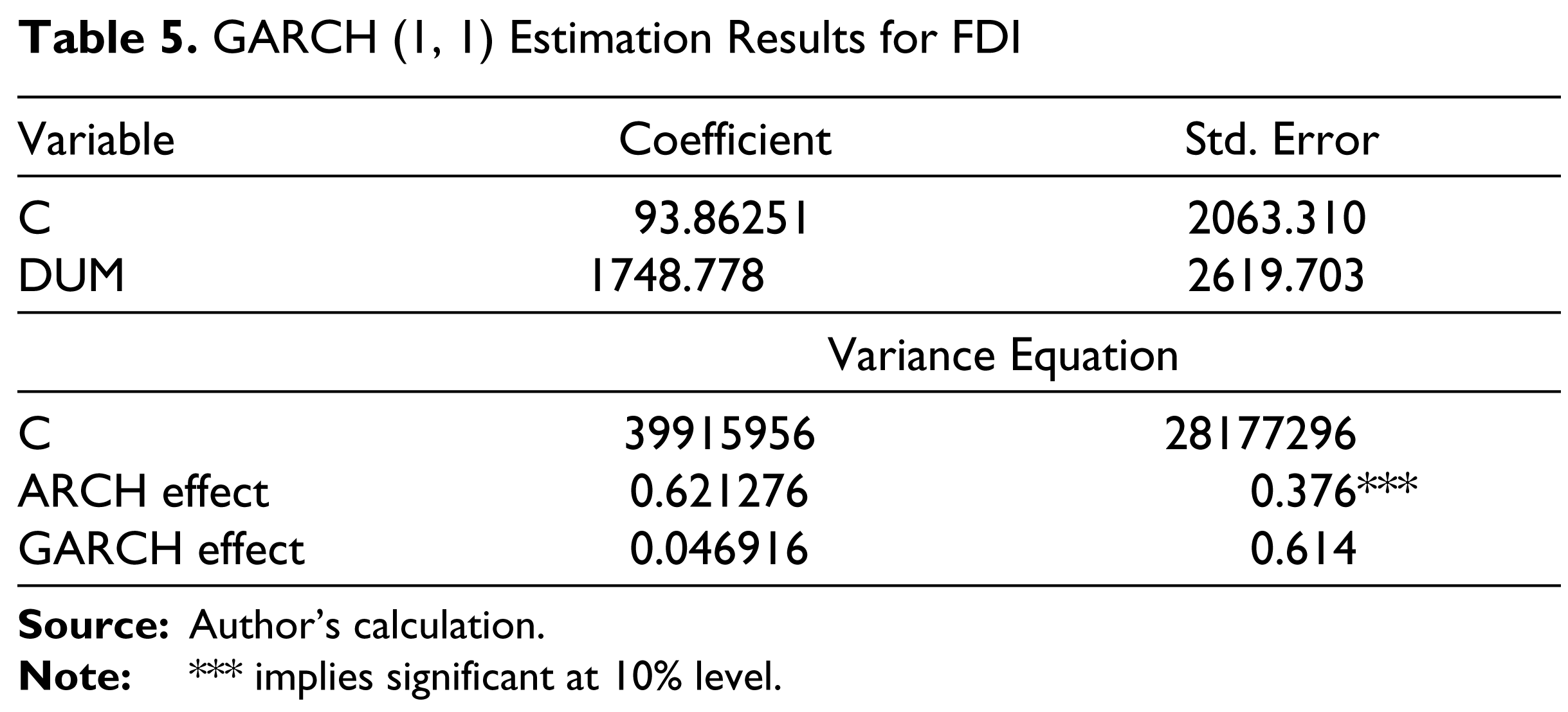
Next we consider the dynamics of volatility in capital inflows as revealed from GARCH (1, 1) estimations. To account for the structural break in the series on capital inflows since 2007.4, a dummy variable (DUM) was introduced into the mean equation, which is set to 0 for the period before 2007.4 and 1 thereafter. The results are reported in Tables 4 to 7. In the variance equation in Table 4, the first three coefficients μ (constant), ARCH term (α) and GARCH term (β) are highly significant and are positive as expected. The significance of α and β indicates that lagged squared disturbance and conditional variance has an impact on the conditional variance. In other words, this means that news about volatility from the previous periods has an explanatory power on current volatility. The sum of the two estimated ARCH and GARCH coefficients α + β is greater than 1, suggesting that shocks to the conditional variance are highly persistent, that is, the conditional variance process is explosive. This implies that large changes in the net capital inflows tend to be followed by large changes and small changes will be followed by small changes which confirm that ‘volatility clustering’ is observed in FINVQ series. Similar findings emerge for PORTFL series as reported in Table 6, but for FDI and COMBOR, the estimated results show that α + β is less than one (Tables 5 and 7). These findings imply that FDI and COMBOR follow a mean reverting variance process. We have estimated the GARCH (1, 1) model separately for the two sub-periods, namely, 1993.2–2007.3 and 2007.4–2012.4, for all the series. From the results, it appears that α + β is almost equal to 1 for all the series in period 1, which implies that the series were mean reverting in period 1. On the other hand, all series appear to be highly persistent in the second period as α + β > 1. Therefore, by using both the static and the dynamic measures of volatility, we can conclude that the volatility of capital inflows increased after the global financial crisis.

Table 4.

GARCH (1, 1) Estimation Results for FINVQ

Variable	Coefficient	Std. Error
C	2553.591	407.957**
DUM	–3049.247	860.102*
Variance Equation
C	11929772	4839875*
ARCH effect	4.042600	0.465*
GARCH effect	0.009033	0.004*

Source: Author’s calculation.

Note: * implies significant at 1% level, ** implies significant at 5% level.

Table 5.

GARCH (1, 1) Estimation Results for FDI

Variable	Coefficient	Std. Error
C	93.86251	2063.310
DUM	1748.778	2619.703
Variance Equation
C	39915956	28177296
ARCH effect	0.621276	0.376***
GARCH effect	0.046916	0.614

Source: Author’s calculation.

Note: *** implies significant at 10% level.

Table 6.

GARCH (1, 1) Estimation Results for PORTFL

Variable	Coefficient	Std. Error
C	–1084.053	1317.413
DUM	1682.799	3052.744
Variance Equation
C	84177985	25506602*
ARCH effect	2.878030	0.9665*
GARCH effect	0.036068	0.032

Source: Author’s calculation.

Note: * implies significant at 1% level.

Table 7.

GARCH (1, 1) Estimation Results for COMBOR

Variable	Coefficient	Std. Error
C	120.2511	546.263
DUM	–103.1639	6476.985
Variance Equation
C	17503408	1710604*
ARCH effect	0.594353	0.457
GARCH effect	0.076618	0.051

Source: Author’s calculation.

Note: * implies significant at 1% level.

Capital Inflows and Policy Trilemma: An Analytical Framework

This section is an extension of Chakraborty (2006). First, we examine the roles of ‘push’ and ‘pull’ factors in determining the capital inflows, using the portfolio balance models. Portfolio balance models aim at explaining how an international investor takes the decision to allocate his or her portfolio across assets marketed in different countries. In these models the differential in the expected rates of return of two countries’ bonds is equivalent to the nominal interest differential minus the expected change in the exchange rate. If the assets of two countries are perfectly substitutable, then this differential in the expected rates of return will be zero. In the finance literature this is known as uncovered interest parity condition. Following the framework of the portfolio balance models, net inflows of capital can be written as a function of the uncovered interest differential and expected depreciation in exchange rate.

Thus,

K_{t} = f ((i_{t} - i_{t} ​ *), Δ e_{t}^{}_{}^{e})

(3)

Where K_t is the net inflows of capital in period t, i_t is the domestic interest rate in period t, i_t* is the US interest rate in period t and e_t^e is the expected rate of change in the exchange rate.

Let us assume that the agents are forward-looking or rational. Then the expected change in the exchange rate is an unbiased predictor of the actual change in the exchange rate. Therefore we can write:

Δ e_{t}^{e} = Δ e_{t}

where Δe_t = actual change in the exchange rate from period t − 1 to t.

Thus equation (3) can be written as:

K_{t} = f ((i_{t} - i_{t} ​ *), Δ e_{t})

(4)

Net inflows of capital also depend on a vector of fundamental determinants which include such variables as current account balance, industrial output, import of capital goods etc. It also depends on some policy variables which change as a response of capital inflows, such as foreign exchange reserves, which has been changing due to the intervention on the foreign exchange market by the Indian government, since the initiation of liberalization of capital inflows. Apart from i*, capital inflows depend on some other push factors such as US industrial production index. Therefore, the augmented portfolio balance model becomes as follows:

K_{t} = f ((i_{t} - i_{t} ​ *), Δ e_{t}, C A B_{t}, F O R E X_{t}, I I P U S_{t})

(5)

Where CAB_t is the current account balance in period t, FOREX_t is the foreign exchange reserves in period t and IIPUS_t is the US industrial production index in period t. The desirable signs of the above variables in equation (5) are as follows: (i_t – i_t*): Higher is the interest rate differential, higher would be capital inflows. Thus the relationship is expected to be positive. Δe_t: Due to capital inflows, exchange rate increases resulting in a negative relationship between Δe_t and K_t. CAB_t: If there is a current account deficit then it may be compensated by capital inflows. Thus the relationship is expected to be negative. FOREX_t: Capital inflows result in an accumulation of foreign exchange reserves. Therefore, if foreign exchange reserves are low, there will be inflows of capital. Thus the relationship is positive. IIPUS_t: If industrial production is high in foreign countries, there will be higher capital inflows in India, resulting in a positive relationship.

For the purpose of estimation, equation (5) becomes as follows:

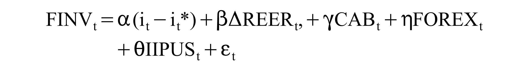
\begin{matrix} F I N V_{t} = α (i_{t} - i_{t} ​ *) + β Δ R E E R_{t}, + γ C A B_{t} + η F O R E X_{t} \\ + θ I I P U S_{t} + ε_{t} \end{matrix}

(6)

where FINV_t represents the net inflows of capital and REER_t is the real effective exchange rate measured by the export based weights.

Next, we test for monetary policy independence from the Real Interest Parity condition. Real Interest Parity is derived from the two cornerstone parity conditions in international macroeconomics, namely, Uncovered Interest Parity and Purchasing Power Parity. Real Interest Parity has significant implication for monetary policy independence. If national real interest rates were bound to converge, monetary policy as a tool of effective macromanagement would be restricted (Mark, 1985). Like Obstfeld, Shambaugh and Taylor (2005), we focus here on the nominal rather than the real interest rate, because nominal interest rate is generally the instrument of the central bank. The Interest Parity condition, considering nominal interest rates, gives the following equation:

i_{t} = i_{t} ​ *

(7)

where i_t is the domestic interest rate in period t and i_t* is the US interest rate.

To test the monetary policy independence, we estimate a long-run relationship between the domestic interest rate and the US interest rate as follows:

i_{t} = α_{0} + β i_{t} ​ * + u_{t}

(8)

Error-correction representation of equation (8) becomes as follows:

Δ i_{t} = α_{1} + γ Δ i_{t} ​ * + λ (i_{t ​ - ​ 1} - δ i_{t - 1} ​ *) + ε_{t}

(9)

where γ indicates the long-run relationship and λ indicates the short-run dynamic adjustment or the error-correction term, λ will be negatively significant to represent that there is short-run dynamic adjustment to maintain long-run equilibrium relationship between the domestic interest rate and the US interest rate. Similar dynamic specification as in equation (4) was also used by Shambaugh (2004) and Obstfeld et al. (2005). A country without monetary policy independence implies that there would be a long-run equilibrium relationship between the domestic interest rate and the US interest rate and any deviation from this long-run relationship would be corrected immediately. Therefore, in this case, γ will be positively significant and λ will be negatively significant.

The relationship between domestic and US interest rates may also be represented in terms of uncovered interest parity condition. The uncovered interest parity condition can be represented as follows:

i_{t} - i_{t} ​ * = E (Δ e_{t} / e_{t}) = E (Δ l e_{t})

(10)

where E(Δe_t/e_t) represents the expected rate of change in the exchange rate in period t and Δle_t is rate of change in log of the exchange rate in period t.

With the assumption of forward-looking agents, equation (10) can be written as:

i_{t} - i_{t} ​ * = Δ l e_{t}

(11)

For empirical estimation of equation (11), one can follow either the approach suggested by Frankel and Okongwu (1995) or the approach suggested by Flood and Rose (2002) and Chinn (2006). Following the first approach, we get the following equation:

i_{t} - Δ l e_{t} = α + β i_{t} ​ * + ε

(12)

Where the null hypothesis is α = 0, β = 1. This signifies perfect capital mobility and perfect substitutability between domestic and foreign assets.

Following the second approach, we get the following estimable equation.

Δ l e_{t} = α + β (i_{t} - i_{t} ​ *) + ε

(13)

Where again, the null hypothesis is α = 0, β = 1.

Capital Inflows and Policy Trilemma: Empirical Estimation

Determinants of Capital Inflows

We estimate equation (6) first by Johansen cointegration method. Then we apply two other methods for testing cointegration, namely, fully-modified OLS (FMOLS) developed by Phillips and Hansen (1990) and dynamic OLS (DOLS) developed by Stock and Watson (1993). The advantage of FMOLS and DOLS methods is that they correct for simultaneity bias among regressors, which has not been taken into account in the Johansen method. Hence, these two methods take into account the problem of endogeneity. Before estimating cointegration, all the three methods require knowledge of the integration properties. We have applied Dickey Fuller (DF), augmented Dickey Fuller (ADF) and Phillips-Perron (PP) tests for testing the presence of unit roots in the variables in equation (6). The results lead us to the conclusion that all variables are stationary in their first differences. (Results are not reported here to save space.)

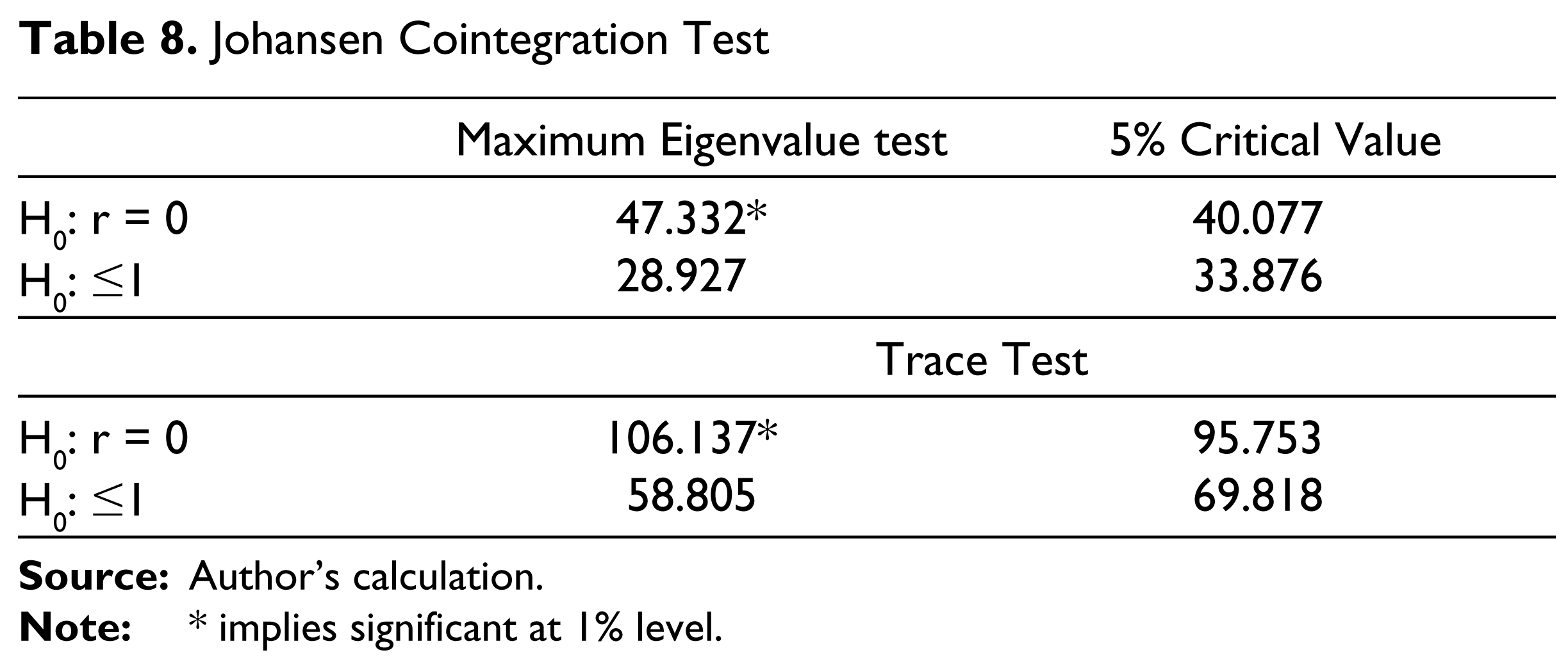
Johansen cointegration test results, considering the entire sample, are reported in Table 8. The eigenvalue test and trace test indicate that there is at least one cointegrating equation at 5 per cent significance level. The cointegrating equations can be interpreted as follows:

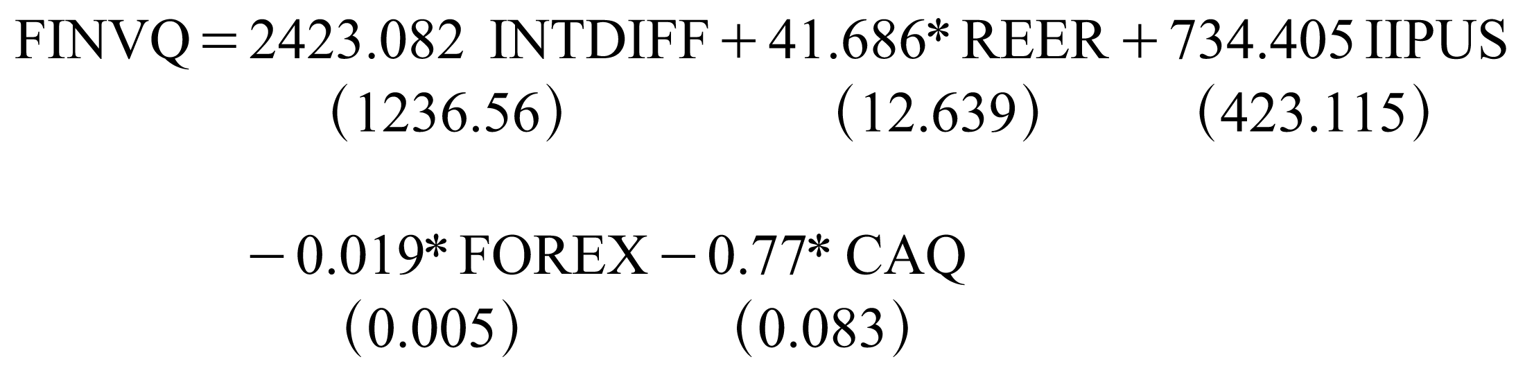
\begin{array}{l} F I N V Q = 2423.082 I N T D I F F + 41.686 ​ * R E E R + 734.405 I I P U S \\ (1236.56) (12.639) (423.115) \\ - 0.019 ​ * F O R E X - 0.77 ​ * C A Q \\ (0.005) (0.083) \end{array}

It implies that as interest differential (INTDIFF) increases, capital inflows will increase but this effect is not significant. On the other hand, as FOREX and CAQ decreases, capital inflows increase and both have significant effects. Again, as the exchange rate increases, that is, currency depreciates, capital inflow increases and this result is significant. The effect of IIPUS is positive and insignificant. Therefore, these results imply that the pull factors and not push factors are important for determining the capital inflows in India.

Table 8.

Johansen Cointegration Test

	Maximum Eigenvalue test	5% Critical Value
H₀: r = 0	47.332*	40.077
H₀: #1	28.927	33.876
Trace Test
H₀: r = 0	106.137*	95.753
H₀: #1	58.805	69.818

Source: Author’s calculation.

Note: * implies significant at 1% level.

Table 9.

FMOLS and DOLS Estimation Results for the Entire Sample

Variable	FMOLS Coefficient	DOLS Coefficient
INTDIFF	–793.890(1150.90)	–1362.692(1364.952)
REER	240.416**(120.716)	342.963*(147.569)
IIPUS	23.786(203.281)	–46.063(260.063)
FOREX	–0.010*(0.004)	–0.015*(0.005)
CAQ	–0.557*(0.044)	–0.524*(0.075)
Constant	–7824.098(28297.22)	–625.127(35205.03)
Adj. R²	0.51	0.68

Source: Author’s calculation.

Note: * implies significant at 1% level, ** implies significant at 5% level.

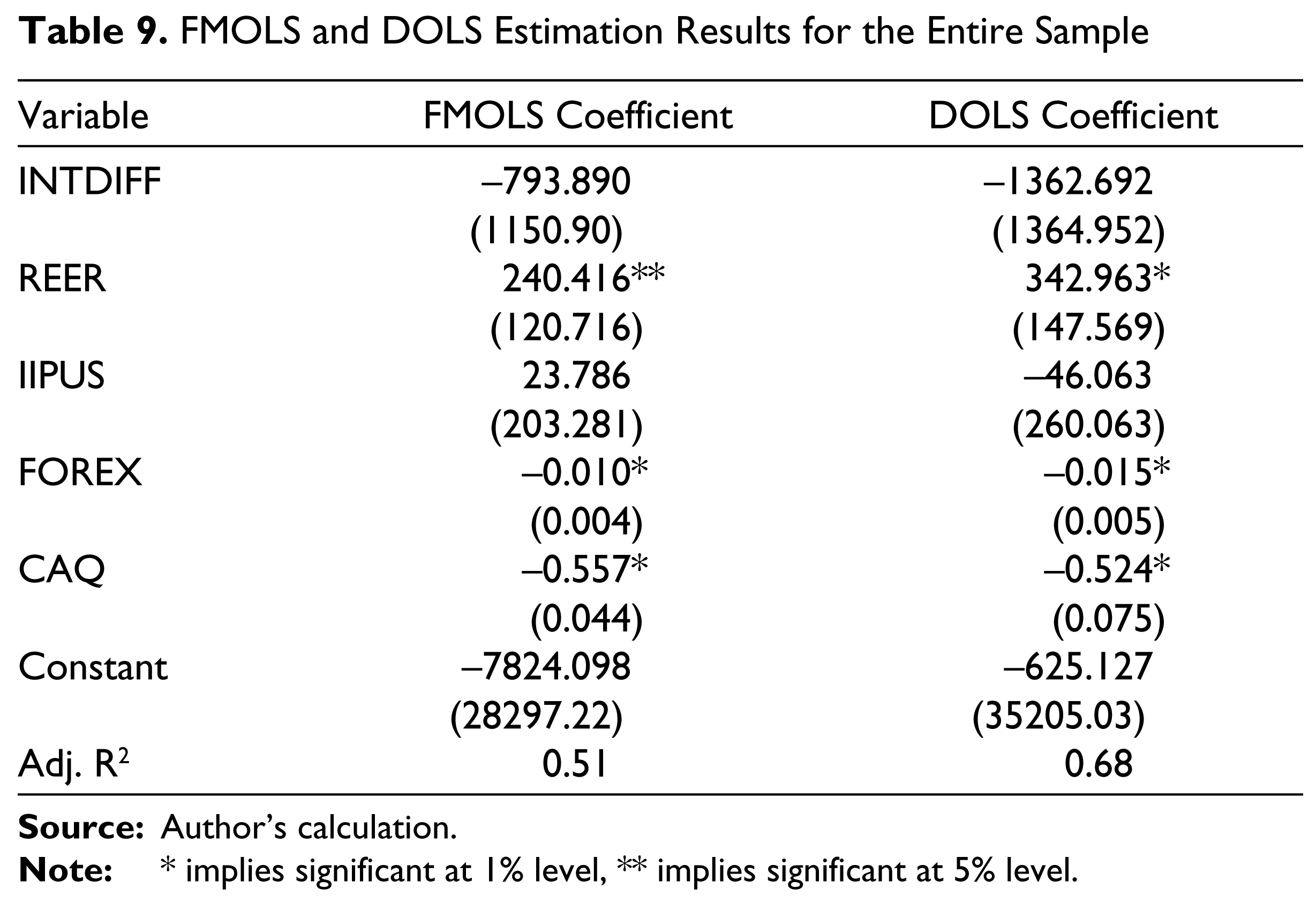
Then we apply the FMOLS and DOLS tests and the results are reported in Table 9. These results show India’s capital inflows to be strongly related to the first difference of REER, FOREX and CAQ. Further, DOLS results also show dependence of capital inflows on the first difference of REER, FOREX and CAQ. These results are consistent with our previous findings from Johansen cointegration results, with once again INTDIFF, IIPUS failing to play a significant role in the determination of India’s capital inflows. Thus, these results also confirm that the pull factors are the major determining factors for capital inflows in India.

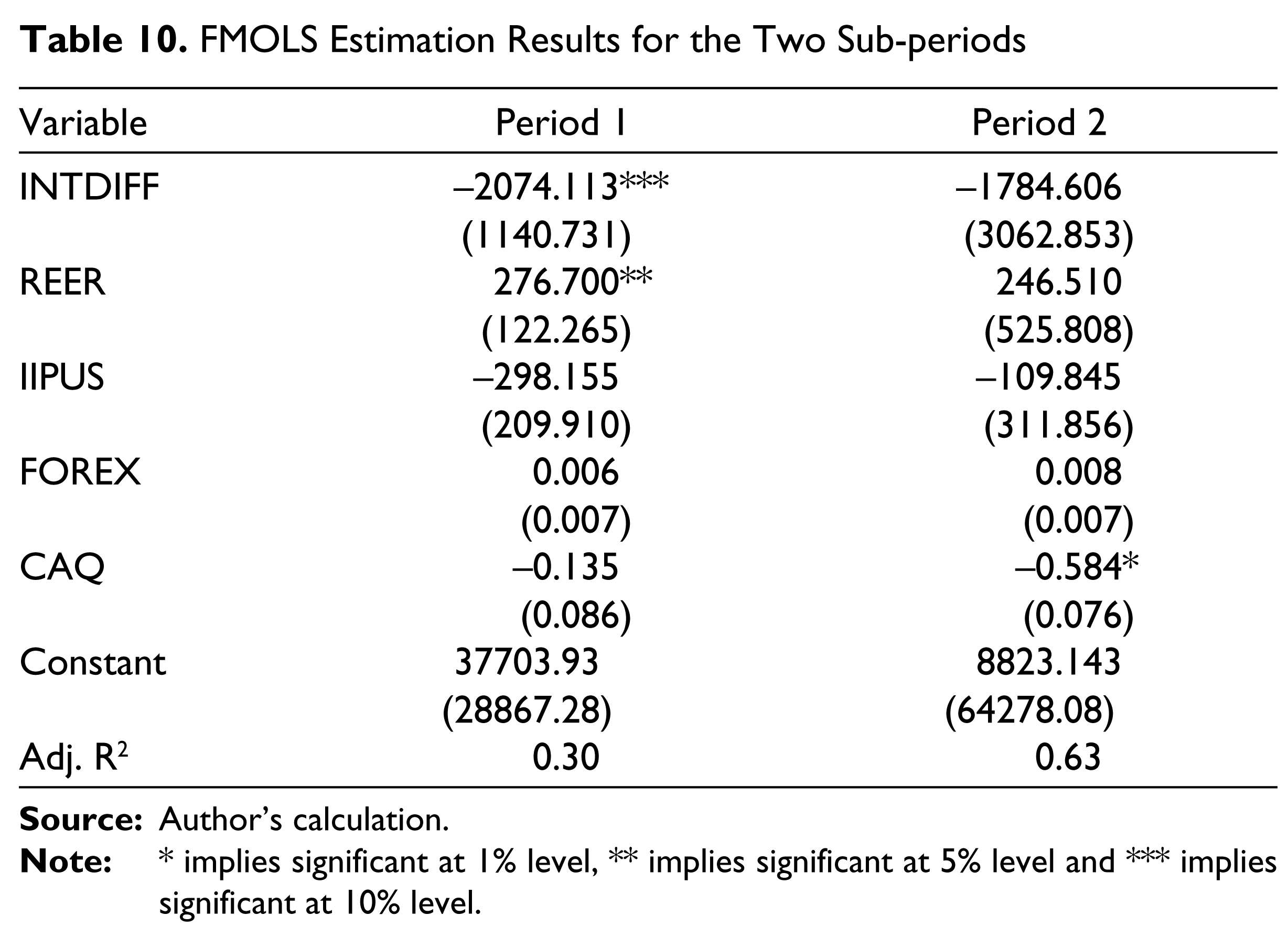
We have also considered the two sub-periods separately and applied FMOLS test for both the periods (Table 10). Because of insufficient data in the second sub-period, the Johansen cointegration test and DOLS test could not be applied. Comparing the results for the two sub-periods, we observe that in the first sub-period INTDIFF and REER are significant while in the second period, only CAQ is significant. Hence, in both the sub-periods, pull factors played the major role in explaining the inflows of capital in India. Further, since the global financial crisis, the only factor which played a major role is current account balance (CAQ) in explaining capital inflows in India. Therefore, due to global financial crisis, there were substantial changes in the roles of the factors playing major role to explain the capital inflows.

Table 10.

FMOLS Estimation Results for the Two Sub-periods

Variable	Period 1	Period 2
INTDIFF	–2074.113***(1140.731)	–1784.606(3062.853)
REER	276.700**(122.265)	246.510(525.808)
IIPUS	–298.155(209.910)	–109.845(311.856)
FOREX	0.006(0.007)	0.008(0.007)
CAQ	–0.135(0.086)	–0.584*(0.076)
Constant	37703.93(28867.28)	8823.143(64278.08)
Adj. R²	0.30	0.63

Source: Author’s calculation.

Note: * implies significant at 1% level, ** implies significant at 5% level and *** implies significant at 10% level.

Monetary Policy Independence

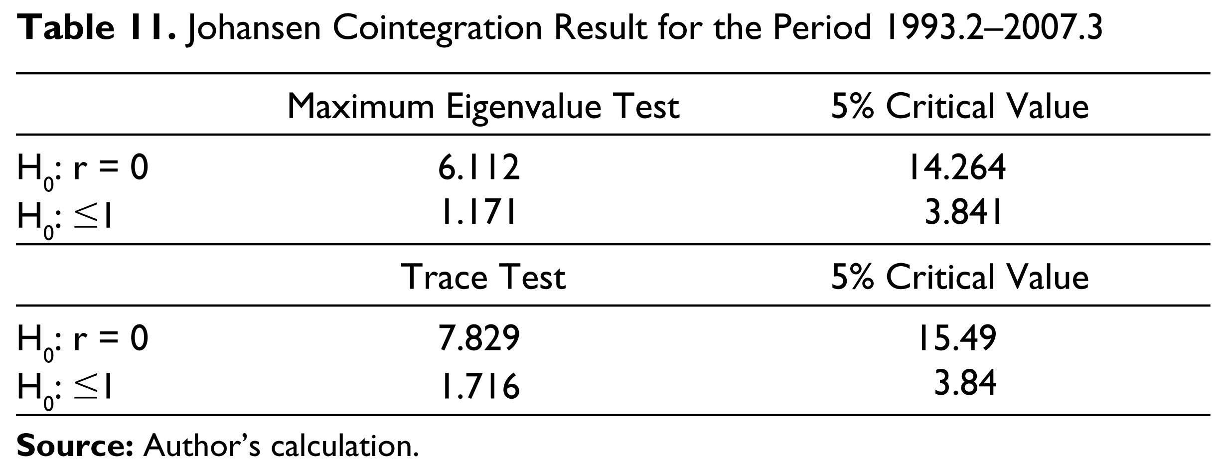
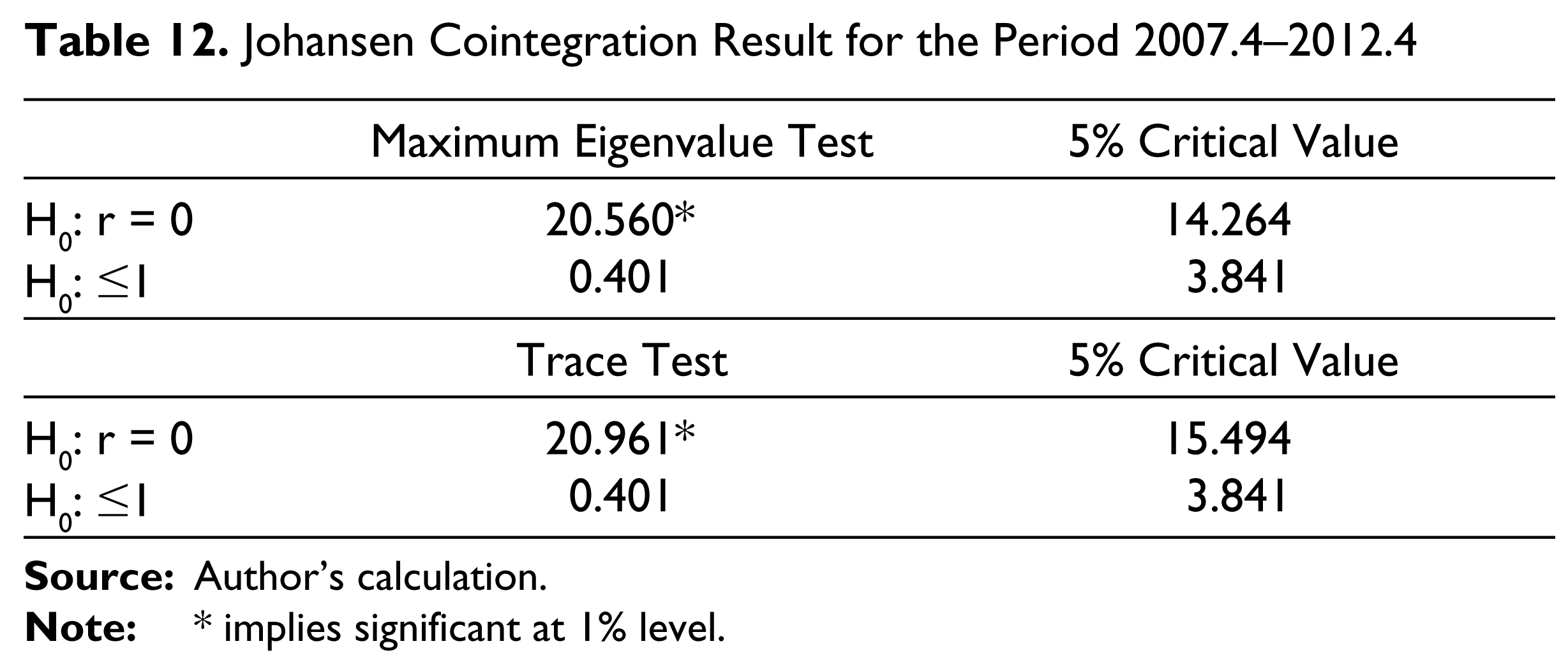
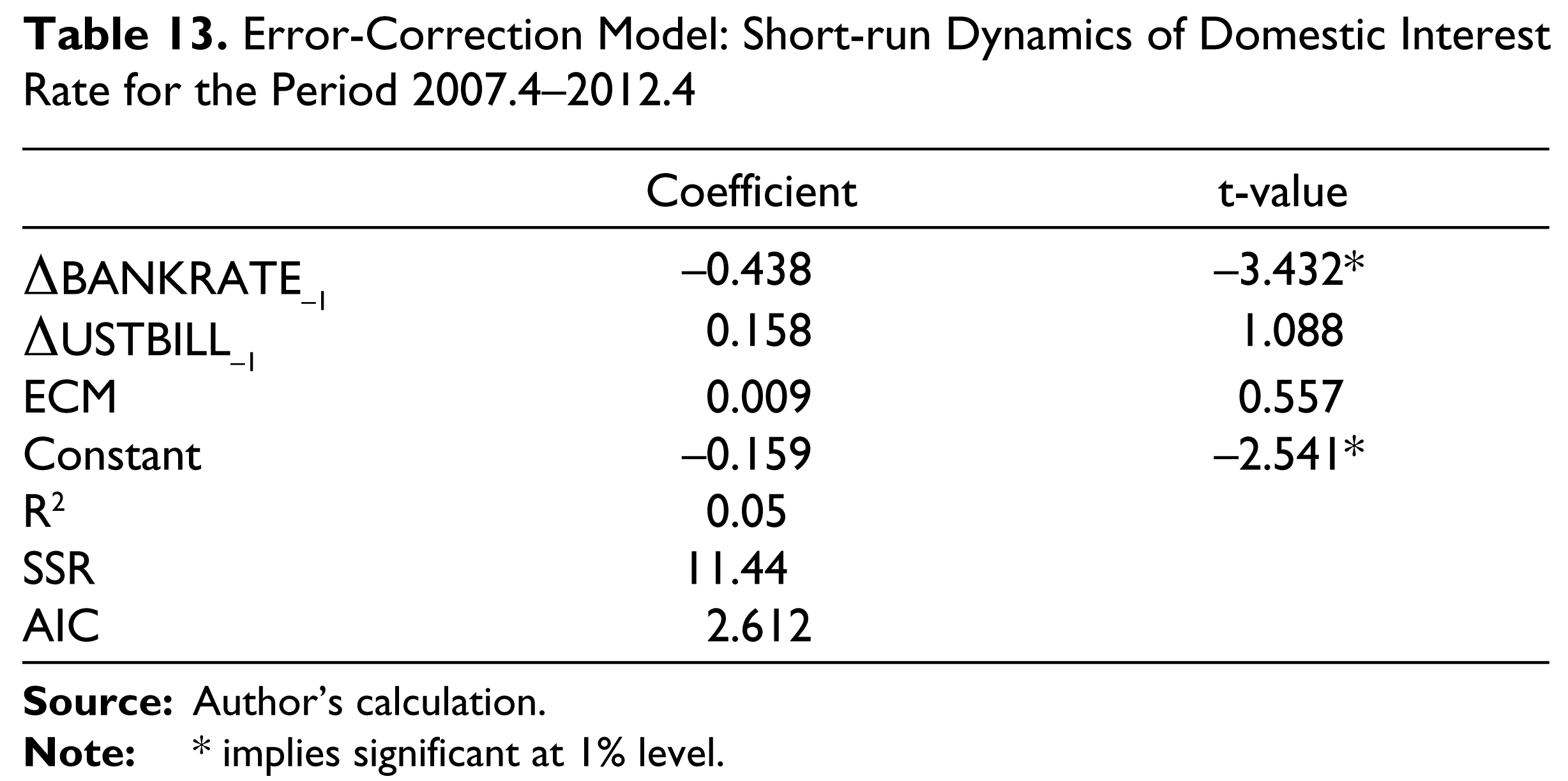
We have applied Johansen cointegration test for testing the presence of cointegration between BANKRATE and USTBILL to draw implications for monetary policy independence. We have applied this test separately for the two sub-periods: 1992.2–2007.3 and 2007.4–2012.4. Johansen cointegration results for the two sub-periods are reported in Tables 11 and 12, respectively. From these results we find that in the first sub-period there is no cointegration between BANKRATE and USTBILL while in the second sub-period there is one cointegration relation between the two. Table 13 reports the error-correction model for the second sub-period. It is evident from Table 13 that the error-correction term is not negatively significant which implies that the short-run dynamic adjustment was not taking place in the second sub-period. Therefore, from the above findings, we can say that in the first sub-period there was independence of monetary policy whereas after the global financial crisis independence of monetary policy was limited.

Table 11.

Johansen Cointegration Result for the Period 1993.2–2007.3

	Maximum Eigenvalue Test	5% Critical Value
H₀: r = 0	6.112	14.264
H₀: #1	1.171	3.841
	Trace Test	5% Critical Value
H₀: r = 0	7.829	15.49
H₀: #1	1.716	3.84

Source: Author’s calculation.

Table 12.

Johansen Cointegration Result for the Period 2007.4–2012.4

	Maximum Eigenvalue Test	5% Critical Value
H₀: r = 0	20.560*	14.264
H₀: #1	0.401	3.841
	Trace Test	5% Critical Value
H₀: r = 0	20.961*	15.494
H₀: #1	0.401	3.841

Source: Author’s calculation.

Note: * implies significant at 1% level.

Table 13.

Error-Correction Model: Short-run Dynamics of Domestic Interest Rate for the Period 2007.4–2012.4

	Coefficient	t-value
ΔBANKRATE_–1	–0.438	–3.432*
ΔUSTBILL_–1	0.158	1.088
ECM	0.009	0.557
Constant	–0.159	–2.541*
R²	0.05
SSR	11.44
AIC	2.612

Source: Author’s calculation.

Note: * implies significant at 1% level.

Table 14.

Domestic Interest Rate Adjusted for Depreciation and US Interest Rate

Period	Constant	USTBILL	Adj R²	DW
1993.2–2007.3	5.199*(0.758)	2.311*(0.180)	0.25	2.14
2007.4–2012.4	6.767*(0.319)	–0.314(0.306)	0.0026	0.706

Source: Author’s calculation.

Note: * implies significant at 1% level.

Table 15.

Foreign Exchange Movement and Interest Differential

Period	Constant	INTDIFF	Adj R²	DW
1993.2–2007.3	0.007(0.016)	0.001(0.003)	–0.016	1.908
2007.4–2012.4	–0.025(0.027)	0.003(0.004)	–0.023	1.24

Source: Author’s calculation.

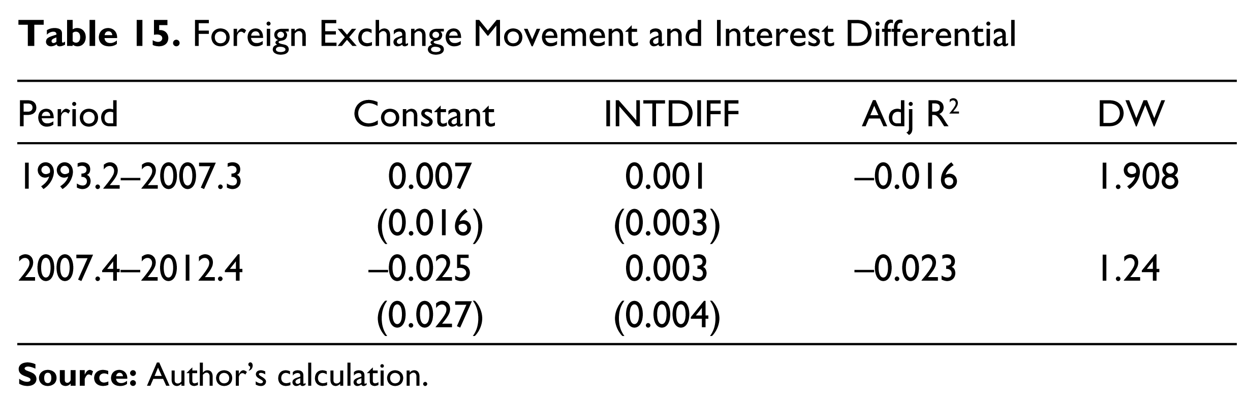
Uncovered Interest Parity

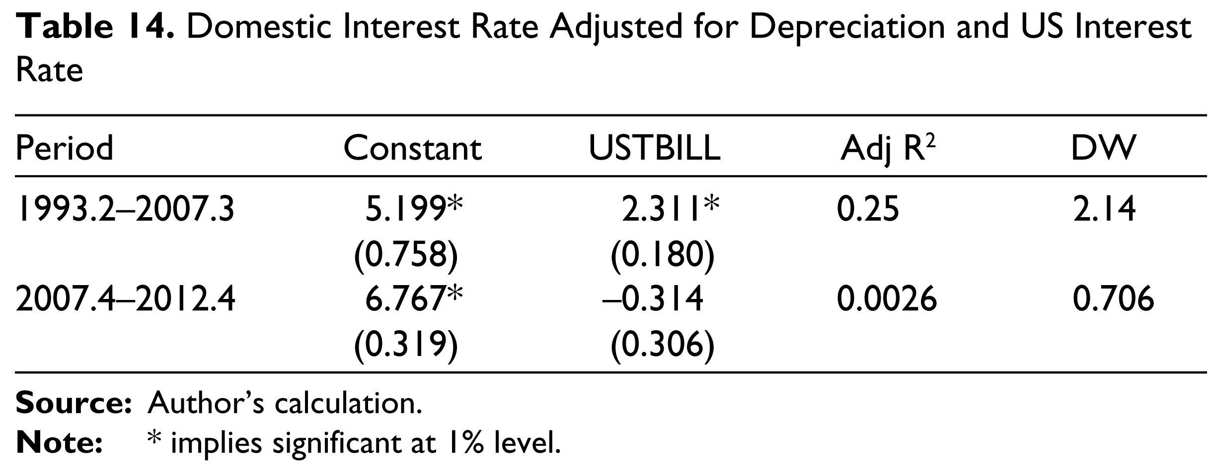
Results on the estimation of uncovered interest parity using alternative approaches are reported in Tables 14 and 15. We find a strong relationship between domestic interest adjusted for depreciation of exchange rate and the US interest rate in period 1 but not in period 2 (see Table 14). On the other hand, we find no strong relationship between depreciation of exchange rate and interest rate differential in both period 1 and period 2 (Table 15). Therefore, the results support the existence of uncovered interest parity in period 1 but not in period 2. Moreover, it may be noted that the coefficient of USTBILL in period 1, is different from the one which signifies that domestic interest rate and interest rate in the US were perfectly substitutable in India during the first period.

The implication of these results could be traced from the theoretical framework developed by Bofinger et al. (2003, 2006), as discussed earlier, which states that monetary policy is effective in a managed floating exchange rate system when capital is perfectly mobile. Following this framework, for maintaining managed floating exchange rate system, the uncovered parity condition should be maintained. In period 1, we observe that uncovered parity condition prevails. Therefore, monetary policy independence might still exist in period 1, under managed floating exchange rate system. Thus the policy trilemma could be resolved in period 1. In the second period, that is, the period after the global financial crisis, we observe that there was no monetary policy independence and hence the absence of the uncovered parity is justified. During this period, owing to the reversal of capital flows, foreign exchange reserves were diminished sharply and targeting the exchange rate through sterilized intervention posed a challenge. In reality, there was an appreciation of the exchange rate which might have led to further capital outflows (Reserve Bank of India Annual Report, 2013. One way to get around this situation would be to have the Reserve Bank of India adjust the interest rates, thereby inducing capital inflows again. Thus, as it became difficult to maintain a stable managed floating system after global financial crisis, with the reversal of capital flows, monetary policy independence had to be abandoned. Therefore, the policy trilemma could be resolved in the period before the global financial crisis but not in the period after the crisis.

Conclusion

In the context of the global financial crisis, this article analyzes the behaviour of capital inflows in India during the period from 1993.2 to 2012.4. It also examines the question how the policy makers have dealt with the ‘policy trilemma’ in a regime of liberalized capital inflows in India. The study finds that the volatility of capital inflows increased after the global financial crisis. Further, due to the global financial crisis, there were substantial changes in the importance of the factors that explain capital inflows. Although the ‘pull factors’ played major roles in both the periods, before and after the crisis, there were significant changes in their roles. In the first sub-period, real effective exchange rate and foreign exchange reserves played the most important roles in determining capital inflows whereas in the second sub-period, it was only current account balance. While dealing with the ‘policy trilemma’ we observed that monetary policy independence was maintained in the period before the crisis which was sacrificed after the crisis.

Footnotes

Acknowledgements

An earlier version of this article was presented at the Workshop on ‘Managing Balance of Payments: Fiscal and Monetary Issues’ organized by the Centre for Advanced Studies, Department of Economics, Jadavpur University held during 5–6 March 2014. The author gratefully acknowledges the suggestions and comments from the participants of the Workshop. I gratefully acknowledge the useful suggestions by the anonymous referee which helped to improve this article.

References

Bofinger

, & Wollmershauser

(2003). Managed floating as a monetary policy strategy. Economics of Planning, 36(2), 81–109.

Bofinger

, Mayer

, & Wollmershauser

(2006). The BMW model: A new framework for teaching monetary economics. The Journal of Economic Education, 37(1), 98–117.

Bollerslev

(1986). Generalized autoregressive conditional heteroscedasticity. Journal of Econometrics, 31(3), 307–327.

Chakraborty

(2006). Capital inflows during the post-liberalisation period. Economic and Political Weekly, 41(2), 14 January, 143–150.

Chinn

M.D.

(2006). The (partial) rehabilitation of interest rate parity in the floating rate era: Longer horizons, alternative expectations and emerging markets. Journal of International Money and Finance, 25(1), 7–21.

Engle

(1982). Autoregressive conditional heteroscedasticity with estimates of the variance of United Kingdom inflation. Econometrica, 50(4), 987–1007.

Fleming

J.M.

(1962). Domestic financial policies under fixed and under floating exchange rates. IMF Staff Papers, 9(November), 369–379.

Flood

R.P.

, & Rose

A.K.

(2002). Uncovered interest parity in crisis. IMF Staff Papers, 49(2), 252–266.

Frankel

J.A.

, & Okongwu

(1995). Liberalized portfolio capital inflows in emerging markets: Sterilization, expectations and the incompleteness of interest rate convergence (Working Paper No. 5156). USA: National Bureau of Economic Research.

10.

Gabriele

, Baratav

, & Parikh

(2000). Instability and volatility of capital flows to developing countries. The World Economy, 23(8), 1031–1056.

11.

Gordon

, & Gupta

(2003). Portfolio flows into India: Do domestic fundamentals matter? (Working Paper No. WP/03/20, 1–38). USA: International Monetary Fund.

12.

Mark

N.C.

(1985). Some evidence on the international equality of real interest rates. Journal of International Money and Finance, 4(2), 189–208.

13.

Mundell

R.A.

(1963). Capital mobility and stabilization policy under fixed and flexible exchange rates. Canadian Journal of Economics and Political Sciences, 29(4), 475–485.

14.

Obstfeld

, Shambaugh

J.C.

, & Taylor

(2005). The trilemma in history: Tradeoffs among exchange rates, monetary policies and capital mobility. Review of Economics and Statistics, 87(3), 423–438.

15.

Osei

, Morissey

, & Lensink

(2002). The volatility of capital inflows: Measures and trends for developing countries (CREDIT Research Paper No. 2/20). United Kingdom: University of Nottingham.

16.

Phillips

P.C.B.

, & Hansen

B.E.

(1990). Statistical inference in instrumental variable regression with I(1) process. Review of Economic Studies, 57(1), 99–125.

17.

Rajan

(2012, September 25). Focus must be on FDI and not on FII inflows. The Hindu.

18.

Reserve Bank of India. (2013a). Annual Report. Reserve Bank of India.

19.

Reserve Bank of India. (2013b). Handbook of Statistics on Indian Economy. Reserve Bank of India.

20.

Shambaugh

J.C.

(2004). The effect of fixed exchange rates on monetary policy. Quarterly Journal of Economics, 119(1), 301–352.

21.

Stock

J.K.

, & Watson

(1993). A simple estimator of cointegrating vectors in higher order integrated systems. Econometrica, 61(4), 783–820.

22.

Taylor

(1986). Modelling financial time series. Chichester: John Wiley and Sons.