The Crowding-in/ out Debate in Investments in India: Fresh Evidence from NARDL Application

Abstract

The purpose of the study is to re-examine the issue of the crowding-in/out effect of public investment on private investment by adopting an improved methodology of the ‘nonlinear autoregressive distributive lag’ (NARDL) model. Taking data from 1970 to 2016, the study finds that public investment crowds-in private investment both in the long-run as well as the short-run. However, the short-run elasticity is statistically more significant and larger in magnitude than the long-run elasticity. It has also been found that macroeconomic uncertainty significantly affects private investment both in the long-run and the short-run. Among other determinants of private investment, we observe foreign direct investment (FDI) inflow, credit flow to the private sector, household savings, real rate of interest and expected output affect private investment significantly. The policy implication of the study calls for the designing of public sector policies that enthuse more private investments. More credit flow to private sectors and FDI in different sectors of the economy should be prioritized.

JEL Codes: E22, H54, C32

Keywords

Crowding-in/out public investment private investment NARDL model India

Introduction

There are different theoretical perspectives—the classical or pre-Keynesian theory, Keynesian theory and the new classical or Ricardian equivalence theory—in the literature on the issue concerning the effects of government spending on private investment. The classical perspective argues that public spending crowds-out private investment, because the hike in government spending and the reduction in tax revenue result in fiscal deficit. Therefore, government spending financed by public borrowings raises the interest rates and lowers the output, leading to the crowding-out of private investment in the economy (Das, 2004; Mohanty, 2018; Şen & Kaya, 2014). However, this theoretical proposition, as illustrated clearly by Das (2004), is based on the assumption of full employment, a condition hardly observed or achieved in developing economies.¹ On the contrary, the Keynesian view, which is most popular in the macroeconomic literature, argues that an increase in government spending stimulates domestic economic activities and causes the crowding in of private investment in the economy. This perspective opines that full employment in the economy exists very rarely. However, the prevalence of under-employment is usual in an economy, and the sensitivity of investment to interest rate would be low (Das, 2004; O’Hara, 2011). The third, new-classical perspective based on the ‘Ricardian equivalence theorem’ suggests that government spending would neither crowd-in nor crowd-out private investment. This is so because the budget deficit being caused by the increased public spending cannot alter the interest rate, thereby not exerting any effect on private investment (Bernheim, 1989).

The empirical validation of this hypothesis involves even greater dissension. It has attracted a great deal of attention among researchers and policymakers across the globe. Many studies, such as Aschauer (1989), Blejer and Khan (1984), Erenburg and Wohar (1995), Mittnik and Neumann (2001), Erden and Holcombe (2005a), Giordano et al. (2007), Ang (2009), Afonso and Jalles (2011) and Andrade and Duarte (2016), found evidence of the crowding-in effect of public investment on private investment in various developed and developing economies. Argimon et al. (1997) examined the empirical relation, in a panel of 14 countries belonging to the Organisation for Economic Cooperation and Development (OECD), between government spending and private spending. The evidence emphasized the existence of a significant crowding-in effect of public investment on private investment, as there was a positive impact of infrastructure on private investment productivity. However, another set of empirical studies negated the hypothesis and found diametrically opposite evidence, thereby concluding in favour of the crowding-out of private investment by public investment (Alesina et al., 2002; Apergis, 2000; Atabev et al., 2018; Mountford & Uhlig, 2005; Voss, 2002; Xu & Yan, 2014). But at the same time, some studies advocated that there is no significant relationship between the two (Badawi, 2003; Kollamparambil & Nicolaou, 2011; Narayan, 2004²; Naqvi & Tsoukis, 2003) or crowding-in during the short-run and crowding-out during long-run (Nguyen & Trinh, 2018). Mahmoudzadeh et al. (2013) conducted an empirical investigation of 23 developed and 15 developing countries using panel data and found evidence of the crowding-out effect in the case of the developed countries and the crowding-in effect for the developing countries.

As regard to the Indian economy, it has undergone a transition from a closed economy to a more flexible and open economy over the years. A major set of reformative actions were adopted in 1991, and the process is still going on. After the reforms, the gap between the two types of investments was bridged by private sector investment. However, the trend of private investments experienced a steady growth over the years (from 16.48% of the GDP in 1990–1991 to 19% in 2000–2001 and 27.45% in 2015), while on the contrary, public sector investments decreased from 11.41 per cent to 7.5 per cent and then slightly increased to 8.66 per cent during the same period. In the pre-reform period, public investments were largely undertaken in the industrial sector, whereas in the post-reform period, they are more concentrated in the infrastructure sector. However, ambiguity still remains in the picture over whether public investments crowd in/out private investments. Empirical testing of this hypothesis reveals that there is no consensus among researchers about the exact relationship between the two. A group of studies, such as Pradhan et al. (1990), Serven (1998), Mitra (2006), Sahu and Panda (2012), Dash (2016) and Mohanty (2018) concluded that public investment crowds-out private investment. However, a few other studies, such as Das (2004), Chakraborty (2007), Muthu (2017) and Barik and Mohanty (2019), contradicted them by concluding a crowding-in effect of public investment on private investment. Interestingly, Bahal et al. (2018), by employing the ‘structural vector error correction model’ (SVECM), found mixed results, that is, crowding-out for the period of 1950–2012 and crowding-in for the period of 1996–2012. This illustrates a further need to re-examine the hypothesis empirically. While there is no consensus among researchers on the exact relationship between the two types of investment, a group of studies, such as Gupta (1992), Parker (1995), Laopodis (2001), Afonso and Aubyn (2010) and Ifeakachukwu et al. (2013), argued that both crowding-in and crowding-out effects are possible depending upon many factors like the empirical model specification, study period, country under consideration, component of government spending, etc. (Şen & Kaya, 2014, p. 635). Hence, here, we take into account the methodological loophole that exists in previous literature. We observe that none of these aforementioned studies have explored the nonlinearity in the relationship between the two types of investment expenditure, which is commonly found in the relationships among many macroeconomic variables. We believe this methodological shortcoming might have been contributing to these confounding results by the different researchers. Keeping this vital point in view, the present study makes an attempt to clear the ambiguity and find a decisive answer to that question of ‘whether the public investment crowds-out or crowds-in private investment in India.’ Hence, the study checks the nonlinearity in the data set, and after confirming the nonlinearity, it adopts an advanced econometric technique, the nonlinear autoregressive distributive lag (NARDL) model, to re-examine the debate of crowding in/out. This model helps us in capturing the possible asymmetries that arise due to the positive and negative shocks in public investment. To the best of our knowledge, none of these aforementioned studies has adopted this model specification to examine this hypothesis.

With this objective, the study is organized into six parts, where the first section sets the background of the study. The second section discusses the trends of investments in India. The theoretical framework is discussed in the third section. Empirical strategies and data sources are mentioned in the fourth section. The fifth section discusses the results, and finally, the study concludes with policy implications.

Trends of Investments in India

The Indian economy has endured the ‘Liberalization, Privatization and Globalization’ (LPG) policy regime during the early 1990s and undergone a transition from a closed economy to a more flexible and open economy. As a consequence of this, a major set of restructuring actions, including the eradication of the licensing system and modification of the ‘monopoly restrictive trade practice’ (MRTP) Act were adopted. When this MRTP Act came into existence, the gap created in the economy was bridged by private sector investments. The private investment trend was observed to have a steady growth from 16.48 per cent of the GDP in 1990–1991 to 30.81 per cent of the GDP in 2010–2011. On the contrary, public sector investments were seen to follow a declining trend from 11.41 per cent to 8.73 per cent of the GDP during the same period. Before the adoption of LPG reforms in the economy, public sector investments were absorbed by the industrial sector, whereas after the reforms, they were mostly undertaken in the infrastructure sector.

Figure 1 depicts the trend of investments in the public sector and private sector as a share of the GDP in the Indian economy, and it is clear from the figure that public investments as a percentage share of GDP showed an increasing trend for the first 26 years of the study, 1970–1986, followed by a declining trend afterwards. However, the trend of private investments is on a steady rise. Therefore, the total investment as a share of the GDP is on an increasing trend. Very recently, private investments faced a slight decline after 2012–2013.

Figure 1.

Source: Central Statistics Office (CSO), Govt. of India.

The Crowding-in/out Hypothesis: Theoretical Framework

The theoretical framework presented here was derived by Blejer and Khan (1984) from the broad framework of the ‘Flexible Accelerator Model’ (FAM) of Jorgenson (1967) and Jorgenson et al. (1971). The basic assumption is that the ‘desired stock of capital is directly proportional to the expected output’. The basic structure of the FAM allows for both reserve constraints and the obvious roles played by monetary, as well as fiscal policies (Erden & Holcombe, 2005a; Muthu, 2017).

The basic assumption of the FAM is that the desired stock of capital is directly proportional to the level of the expected output (Akber & Paltasingh, 2019; Aschauer, 1989; Erden & Holcombe, 2005b; Muthu, 2017), and is stated as below:

K P_{t}^{*} = a Y_{t}^{e} ​ ​,

(1)

where $K P_{t}^{*}$ is the desired capital stock that the private sector might have in the future time t; $Y_{t}^{e}$ is the corresponding expected output. Factors such as the changing economic conditions affect $K P_{t}^{*}$ . Thus, the model does fit into the flexible accelerator framework. As we know, there lies a lag in the adjustment process of actual investment to come up. Because it takes time to plan, construct and put in new capital. Hence, the actual level of capital stock is supposed to adjust as per the variance between the current desired stock at time t and the previously realized capital stock, and is expressed as:

Δ K P_{t} = - β (K P_{t}^{*} - K P_{t - 1})

(2)

K P_{t} = β K P_{t}^{*} + (1 - β) K P_{t - 1},

(3)

where KP_t is the actual capital stock, ΔKP_t is the net private investment and β ϵ [0,1] is the coefficient of adjustment.

Moreover, the dynamic structure of the private investment can be explained by the one-period quadratic cost adjustment function (Erden & Holcombe, 2005a; Salmon, 1982) as:

β {(K P_{t} - K P_{t}^{*})}^{2} + (1 - β) {(K P_{t} - K P_{t - 1}^{*})}^{2},

(4)

where $β {(K P_{t} - K P_{t}^{*})}^{2}$ is the cost of disequilibrium and $(1 - β)$ ${(K P_{t} - K P_{t - 1}^{*})}^{2}$ is the cost of adjustment towards equilibrium. To obtain the partial adjustment mechanism, we have to minimize the cost of equilibrium with respect to actual capital stock, which renders Equation (5) as:

K P_{t} - K P_{t - 1} = β (K P_{​}^{*} - K P_{t - 1}),

(5)

where 0 ≤ β ≤ 1 and the actual private capital stock is supposed to adjust to the difference between the desired stock of capital at time t and the previously observed stock at a time (t − 1).

In developing countries, usually the data is available and accessible merely in the gross terms together with depreciation. Hence, we can define gross private investment IP_t equal to net investment along with the depreciation of the previous period’s capital stock (Muthu, 2017) as:

I P_{t} = Δ K P_{t} + δ K P_{t - 1}

(6)

I P_{t} = K P_{t} - K P_{t - 1} + δ K P_{t - 1}

(7)

By making use of the standard lag operator, that is, $L K P_{t} = K P_{t - 1},$ the above equation can be written as:

I P_{t} = (1 - (1 - δ) L) K P_{t} .

(8)

Applying the partial adjustment mechanism to the gross private investment, we get

I P_{t} - I P_{t - 1} = β (I P_{t}^{*} - I P_{t - 1}) .

(9)

To facilitate more dynamics into the model, it is supposed that the speed of adjustment (β) between the currently desired and the observed previous private investment is determined by the public investment and other relevant factors such as lending rate, credit flow to the private sectors, inflow of foreign direct investment (FDI), domestic savings and so on. Following Price (1996), Erden and Holcombe (2005a), the rate of adjustment (β) is considered as a linear function of public investment and other factors as:

β = γ_{0} + [\frac{1}{(I P_{t}^{*} - I P_{t - 1})}] (γ_{1} I G_{t} + γ_{2} Z_{t}),

(10)

where IG is the public investment and Z is the vector of other relevant factors. If the gross public investment is complementary to the gross private investment, then it speeds up the adjustment mechanism, and vice versa. Hence, finally clubbing together Equations (9) and (10) renders Equation (11) as:

I P_{t} - γ_{0} (I P_{t}^{*} - I P_{t - 1}) + I P_{t - 1} + γ_{1} I G_{t} + γ_{2} Z_{t} .

(11)

Note that Equation (8) in a steady state can be expressed as $I P_{}^{*} = (1 - (1 - δ) L) K P_{t}^{*} .$ Substituting this for $I P_{t}^{*}$ in Equation (11) and utilizing Equation (1), we obtain the basic ‘Dynamic Accelerator Model’ for gross private investment as:

I P_{t} = γ_{0} [1 - (1 - δ) L] Y_{t}^{e} + (1 - γ_{0}) I P_{t - 1} + γ_{1} I G_{t} + γ_{2} Z_{t} .

(12)

The above equation has an edge over the original Equation (1), and it is also consistent with the original capital stock model explained in Equation (1) and Equation (2), as it does not necessitate any data on the net investment or stock of capital (Erden & Holcombe, 2005a, b; Muthu, 2017). Thus, we can apply this model to the gross investment data available in many developing countries like India. The ‘γ₁’ coefficient captures the impact of public investment on private investment, which could be positive or negative depending upon whether it is complementary or substitutable to private investment. The coefficient $Y_{t}^{e}$ captures the acceleration effect, and it is expected to be positive. Private investment is also influenced by several other factors, such as the cost of credit, availability of financing, level of domestic savings, economic uncertainty, foreign direct investment and so on. Several researchers suggested that under the conditions of uncertainty and irreversibility, uncertainty should be included in the model, as it affects private investment both ways: it does affect the long-run steady equilibrium as well as the short-run steady equilibrium of the private investment (Muthu, 2017; Price, 1996).

Equation (12) is expressed in the form of a log-linear model below:

\begin{matrix} L n I P_{t} = α_{0} + β_{1} \ln I P_{t - 1} + β_{2} \ln I G_{t} + β_{3} \ln C R D T_{t} + \\ β_{4} \ln F D I_{t} + β_{5} \ln S A V_{t} + β_{6} \ln I N F V_{t} + \\ β_{7} \ln L R_{t} + β_{8} \ln Y_{t}^{e} + ε_{t}, \end{matrix}

(13)

where IP_t is the private sector fixed capital formation, which consists of the gross fixed capital formation and IG_t is the public sector fixed capital formation. CRDT_t is the credit flow to the private sector, SAV_t the total savings, INFV_t the inflation volatility, LR_t the lending rate, $Y_{t}^{e}$ . the expected output and ε_t the error term.

Materials and Methods

In this study, the NARDL approach has been applied, since it is an appropriate method applicable when there is a varied order of stationarity of variables (Akber & Paltasingh, 2019). Again, it captures the nonlinear relationship that has not been explored. First, all the unit root tests were conducted with the intercept and the intercept plus trend, in order to check the stationarity of the data, and then the NARDL approach was applied and other diagnostic tests were conducted.

The NARDL Approach

The NARDL model, developed by Shin et al. (2014), is an extended and advanced version of the autoregressive distributive lag (ARDL) model proposed by Pesaran et al. (2001). It uses negative and positive shocks and also captures the possible asymmetries in the short-run as well as the long-run relationship. The public investment is decomposed into positive and negative shocks as:

{\begin{cases} I G + = \sum_{j = 1}^{t} M a x (Δ I G_{j}^{+}, 0) \\ I G - = \sum_{j = 1}^{t} M a x (Δ I G_{j} -, 0) \end{cases}

(14)

Incorporating Equation (14), the NARDL model can be estimated as:

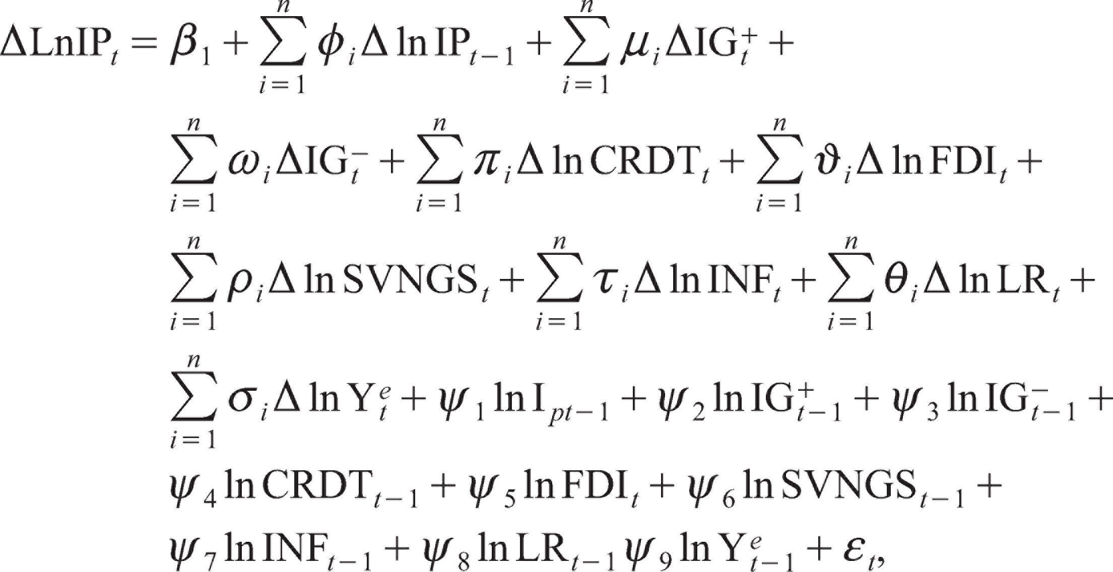
\begin{array}{l} \begin{matrix} Δ L n I P_{t} = β_{1} + \sum_{i = 1}^{n} ϕ_{i} Δ \ln I P_{t - 1} + \sum_{i = 1}^{n} μ_{i} Δ I G_{t}^{+} + \\ \sum_{i = 1}^{n} ω_{i} Δ I G_{t}^{-} + \sum_{i = 1}^{n} π_{i} Δ \ln C R D T_{t} + \sum_{i = 1}^{n} ϑ_{i} Δ \ln F D I_{t} + \\ \sum_{i = 1}^{n} ρ_{i} Δ \ln S V N G S_{t} + \sum_{i = 1}^{n} τ_{i} Δ \ln I N F_{t} + \sum_{i = 1}^{n} θ_{i} Δ \ln L R_{t} + \end{matrix} \\ \begin{matrix} \sum_{i = 1}^{n} σ_{i} Δ \ln Y_{t}^{e} + ψ_{1} \ln I_{p t - 1} + ψ_{2} \ln I G_{t - 1}^{+} + ψ_{3} \ln I G_{t - 1}^{-} + \\ ψ_{4} \ln C R D T_{t - 1} + ψ_{5} \ln F D I_{t} + ψ_{6} \ln S V N G S_{t - 1} + \\ ψ_{7} \ln I N F_{t - 1} + ψ_{8} \ln L R_{t - 1} ψ_{9} \ln Y_{t - 1}^{e} + ε_{t}, \end{matrix} \end{array}

(15)

where Δ is the difference operator, β_l denotes the constant term and ‘ln’ stands for natural logarithm, as all variables are transformed into a natural logarithm. ψ_s are the long-run parameters, while ϕ_i, μ_i, ω_i, ϑ_i, θ_i, π_i, ρ_i, τ_i and σ_i are the short-run parameters. ε_t is the residual term, which is assumed to be normally distributed. The null hypothesis of no cointegration among the variables in the equation is H₀: ψ₁ = ψ₂ = ψ₃ = ψ₄ = ψ₅ = ψ₆ = ψ₇ = ψ₈ = ψ₉ = 0 against the alternative hypothesis H₁: ψ₁ ≠ ψ₂ ≠ ψ₃ ≠ ψ₄ ≠ ψ₅ ≠ ψ₆ ≠ ψ₇ ≠ ψ₈ ≠ ψ₉ ≠ 0, which implies a long-run cointegration among the variables (Ahmad et al., 2019; Rahman et al., 2019). If the calculated F-statistic is more than the respective upper critical values, then we reject H₀ of no cointegration, and it shows the existence of a long-term relationship between the variables. However, if the calculated F-statistic is less than the respective lower bound critical values, then we do not reject the H₀ and conclude that there is no cointegration among the variables. However, if the F-statistic falls between the lower bound and the upper bound, then the result is inconclusive.

The next step is to obtain short-run dynamic parameters by estimating an error correction model (ECM) with the long-run estimates. The short-run model can be estimated by using the following equation:

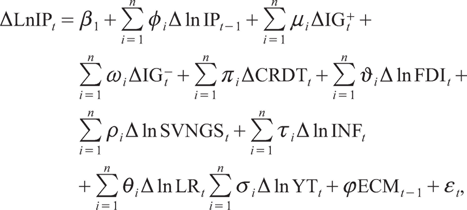
\begin{array}{l} \begin{matrix} Δ L n I P_{t} = β_{1} + \sum_{i = 1}^{n} ϕ_{i} Δ \ln I P_{t - 1} + \sum_{i = 1}^{n} μ_{i} Δ I G_{t}^{+} + \\ \sum_{i = 1}^{n} ω_{i} Δ I G_{t}^{-} + \sum_{i = 1}^{n} π_{i} Δ C R D T_{t} + \sum_{i = 1}^{n} ϑ_{i} Δ \ln F D I_{t} + \end{matrix} \\ \begin{matrix} \sum_{i = 1}^{n} ρ_{i} Δ \ln S V N G S_{t} + \sum_{i = 1}^{n} τ_{i} Δ \ln I N F_{t} \\ + \sum_{i = 1}^{n} θ_{i} Δ \ln L R_{t} \sum_{i = 1}^{n} σ_{i} Δ \ln Y T_{t} + φ E C M_{t - 1} + ε_{t}, \end{matrix} \end{array}

(16)

where ϕ_i, μ_i, ω_i, π_i, ϑ_i, ρ_i, τ_i, θ_i, and σ_i are the short-run dynamic parameters to equilibrium, which show the short-run multiplier effect with respect to all the relevant variables. The error correction term (ECM_t-1) indicates the speed of adjustment back to the long-run equilibrium after a short-run shock.

Data and Variables

For this study, data from the different volumes of National Account Statistics (NAS) published by the ‘Central Statistics Office’ (CSO) and the Handbook of Statistics on Indian Economy by the ‘Reserve Bank of India’ (RBI) are taken into consideration. Certain data series are also taken from World Bank data. All the data are taken for the period from 1970 to 2017. Both types of investments are taken in crores of Indian rupees (₹) at the 2011–2012 prices. The public investment is inclusive of all central, state and local governments’ gross fixed capital formation. The private investment is inclusive of all the investments made by individuals or groups of individuals in the private sector. Following Erden and Holcombe (2005a) and Akber and Paltasingh (2019), the estimated log values of the GDP at the 2011–2012 prices from first-order autoregressive (AR) processes are taken as a proxy for the expected output. As we know that the macroeconomic uncertainty is not directly observable, the observations are spawned using generalized autoregressive conditional heteroscedasticity (GARCH). Inflation is frequently taken as a summary measure of macroeconomic uncertainty, and its volatility is quite unpredictable. Therefore, it has been an imperative indicator of over-all macroeconomic uncertainty. To find this inflation volatility, the wholesale price index for all the commodities from 1970 to 2016 has been used.

Empirical Results

Unit Root and Nonlinearity Test

Table A1 presents the results of unit root tests (Augmented Dickey–Fuller [ADF] and Phillips–Perron [PP] tests) with both intercept and trend. It is observed that variables like inflation volatility rate (INFV), lending rate (LR) and expected output (Y^e) are stationary at level I(0), and the rest of the variables are stationary at the first difference I(1). Thus, we have a mixed order of stationarity of variables. The application of these unit root tests (ADF and PP tests) has one limitation of causing spurious regression by ignoring the structural breaks. To overcome this, we have used the Zivot–Andrews test. Table A2 depicts the results of the unit root test with structural breaks, which confirms the mixture of stationarity of variables. This allows us to use the NARDL model.

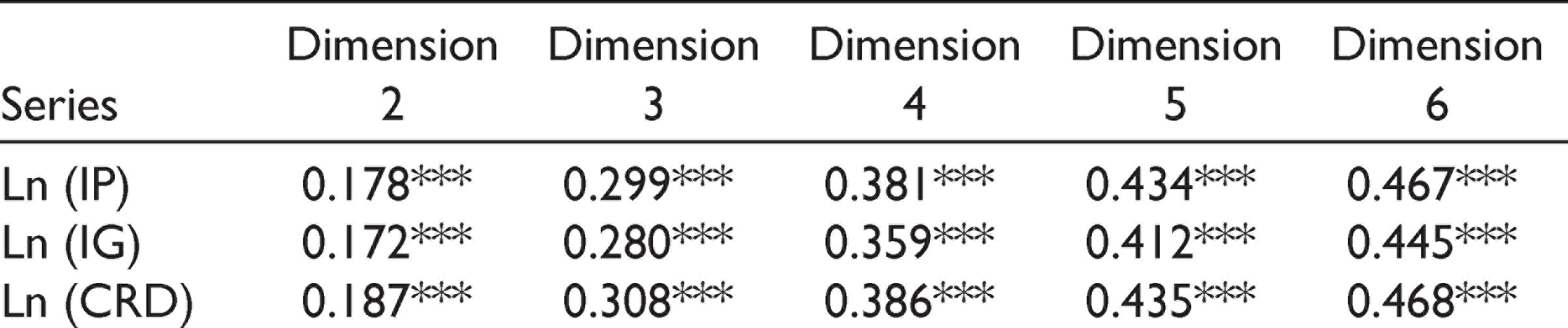
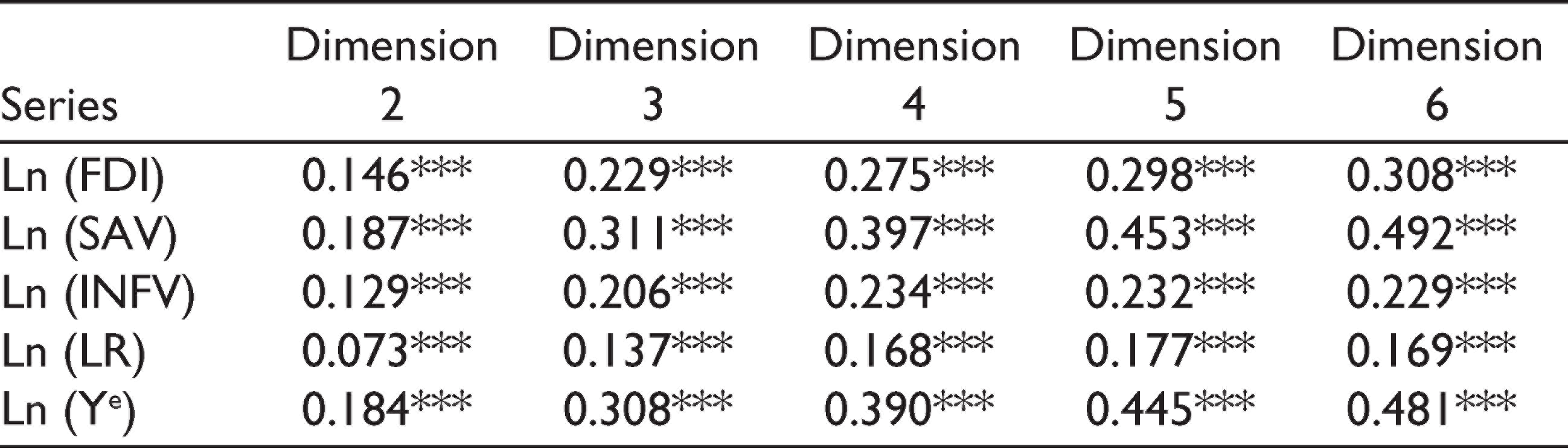
Again, the Brock-Dechert-Scheinkman (BDS) test, as developed by Brock et al. (1996), has been used to check the nonlinearity in the series. Table A3 shows the results of the BDS test, and the results clearly show that the series is not ‘identically and independently distributed’ (IID). After confirming the nonlinearity in the model, we move to the NARDL model.

Testing of Asymmetries

Table 1 depicts the Wald test results of the long-run and short-run asymmetries. The Wald test results confirm the existence of asymmetry by rejecting the null hypothesis of symmetries in both the long-run and the short-run.

Table 1.

Results of Long-run and Short-run Asymmetries (Wald test)

Test	F-statistic	Probability	Decision
W_LR	58.72	0.00	Asymmetries
W_SR	13.33	0.00	Asymmetries

Source: Authors’ estimation.

Notes: W_LR and W_SR indicate the Wald test for long-run and short-run asymmetries, respectively. The null hypothesis (H₀) for this test is the existence of symmetries against the alternative hypothesis (H₁) of asymmetries.

Results of the NARDL Model

Table 2 presents the results of the long-run elasticities of the NARDL model, which clearly show that the estimated coefficients are positive for the positive components and negative for the negative components of public investment. In other words, positive shocks or increases in public investment affect the private investment positively and significantly, while the negative shocks or decreases affect it negatively. The values of elasticities are 0.501(−2.253) for public investment increase (decrease), indicating that with a 10 per cent increase (decrease) in public investment may induce an increase (decrease) in private investment by 5.01 per cent (−22.53%), respectively. From the magnitude of the elasticities, it is found that negative shocks have stronger effects than positive shocks. The coefficients are statistically significant at the 5 per cent level of significance. Among other variables, domestic credit flow, FDI inflow and the expected output have significant positive impacts on private investment. Their estimated elasticities are 0.94, 0.02 and 0.09, respectively. The elasticities of domestic credit flow to private sectors and FDI inflow are statistically significant. However, no significant impact is observed in the case of the expected output. Savings, inflation volatility rate and lending rate have a negative and significant impact on private investments in India. The negative impact of domestic savings on private investment goes against intuition, but it is possible, because the investments in the Indian economy are domestic demand-driven. Hence, higher savings implies lower spending, subject to the assumption that the household income remains constant or increases slowly, at a rate lower than that of inflation. Therefore, it is aggregate spending rather than savings that stimulates investment. The macroeconomic uncertainty in the economy adversely affects the macroeconomic environment and discourages investors. The F-statistic value of the nonlinear bound test is 9.09, which is higher than the lower bound and upper bound critical values at the 1 per cent level of significance. This indicates the existence of co-integration among the variables in the long run.

Table 2.

NARDL Estimates of Long-run Elasticities

Variables	Coefficient	Std. Error	Prob.
Ln(IG)⁺	0.501**	0.210	0.024
Ln(IG)^–	−2.253***	0.404	0.000
Ln(CRDT)	0.948***	0.199	0.000
Ln(FDI)	0.028*	0.015	0.068
Ln(SAV)	−0.619***	0.191	0.003
Ln(INFV)	−0.002***	0.001	0.001
Ln(LR)	−0.921***	0.188	0.000
Ln(Y^e)	0.096	0.229	0.677
Constant	3.906***	1.397	0.009
Bound test F-statistic	9.094

	Critical values of the bound test
Level of significance	Lower bound 1(0)	Upper bound 1(1)
10%	1.85	2.85
5%	2.11	3.15
1%	2.62	3.77

Source: Authors’ estimation.

Notes: ***, ** and * Indicate significance at 1%, 5% and 10%, respectively.

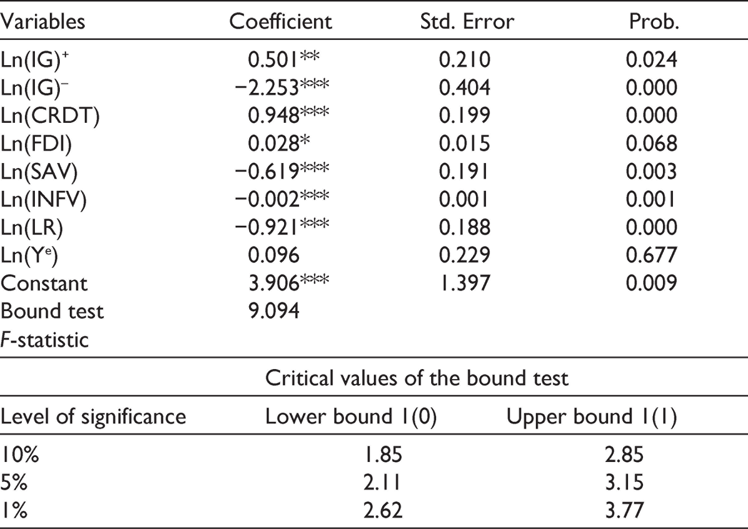
Table 3 shows the results of the short-run elasticities of the NARDL model. The short-run results also show that the estimated coefficients of elasticity of public investments are positive for positive shocks and negative for negative shocks, indicating thereby that an increase (decrease) in public investments affects private investments accordingly. The values of elasticities are 0.458 (−1.055), which indicate that with a 10 per cent increase (decrease) in public investment, private investment responds positively (negatively) by 4.58 per cent (−10.55%), respectively. The coefficients of elasticities are statistically highly significant at the 1 per cent probability level. Hence, looking at both the long- and short-run results, it is quite clear that public investment crowds-in private investment in India. This result is supported by earlier studies like Chakraborty (2007), Muthu (2017) and Barik and Mohanty (2019), who concluded in favour of the crowding-in effect of public investment on private investment. Among other variables, domestic credit flow, FDI and expected output have a positive impact on private investments, but no significant impact is observed in the case of expected output. Savings and inflation volatility rate are observed to have a negative impact. However, no significant impact of the lending rate is observed in the short run.

Table 3.

NARDL Estimates of Short-run Elasticities

Variable	Coefficient	Std. Error	Prob.
ΔLn (IP(−1))	0.086	0.156	0.583
ΔLn (IG)⁺	0.458	0.169	0.011
ΔLn (IG)⁻	−1.055	0.472	0.033
ΔLn (CRD)	0.866	0.207	0.001
ΔLn (FDI)	0.025	0.014	0.081
ΔLn (SAV)	−0.566	0.183	0.004
ΔLn (INFV)	−0.020	0.001	0.000
ΔLn (LR)	−0.093	0.094	0.331
ΔLn (Y^e)	0.088	0.217	0.688
ECM (−1)	−0.694	0.127	0.000
Adjusted R-squared	0.92
D–W statistic	2.26

Source: Authors’ own estimation.

Notes: ***, ** and * Indicate significance at 1%, 5% and 10%, respectively.

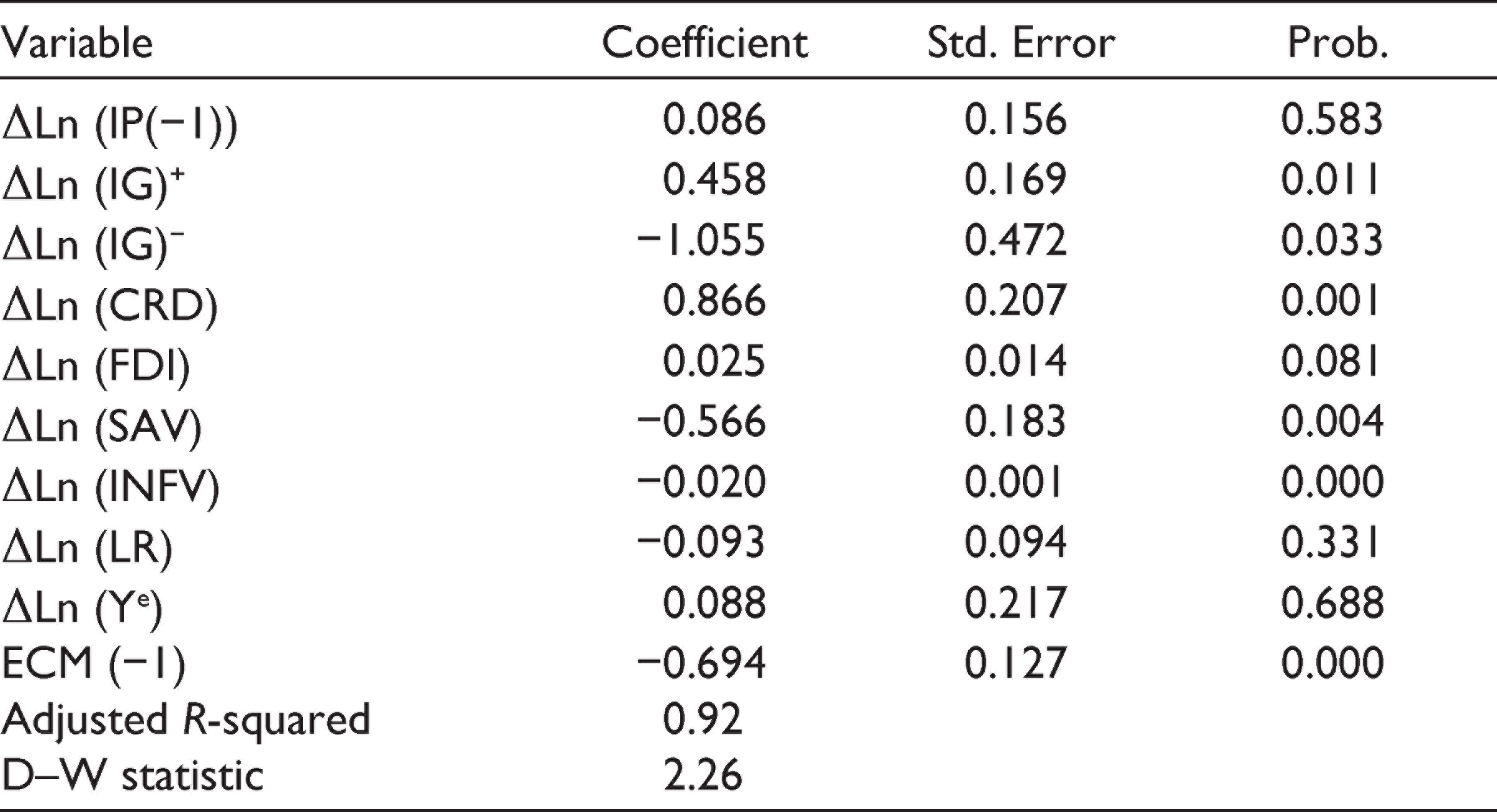
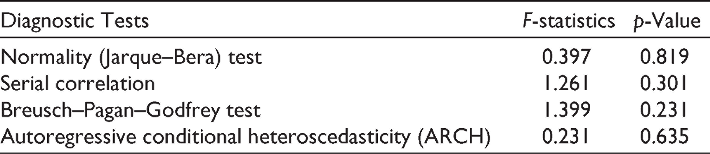
The lagged value of ECM is negative (−0.694) and statistically highly significant at the 1 per cent level. This means that when there is a deviation in private investment from its equilibrium value, around 70 per cent gets corrected every year. Hence, the speed of adjustment is quite fast. The value of adjusted R-squared is 0.92, indicating a good fit of the model. The value of the Durbin–Watson statistic is greater than the R-squared value, indicating the non-existence of spurious regression. Table 4 depicts the results of various diagnostic tests (normality, serial correlation and heteroscedasticity), and we observe that all the probability values are greater than 0.05, indicating that the model passes through all the diagnostic tests. There are no biases in the estimated model and it is well specified empirically.

Table 4.

Various Diagnostic Tests

Diagnostic Tests	F-statistics	p-Value
Normality (Jarque–Bera) test	0.397	0.819
Serial correlation	1.261	0.301
Breusch–Pagan–Godfrey test	1.399	0.231
Autoregressive conditional heteroscedasticity (ARCH)	0.231	0.635

Source: The authors’ estimation.

Stability Tests and Dynamic Multiplier Graph

Cumulative sum (CUSUM) and cumulative sum of squares (CUMSUMQ) tests have been used to check the stability of the model. Figures A1 and A2 in the Appendix show that our model is stable, as the estimated line is within the boundaries of critical values at the 5 per cent level of significance. The dynamic multiplier graph (Figure A3) in the Appendix is used to check the asymmetry due to the positive and negative shocks. The curve depicts the asymmetric adjustments of public investments to the positive and negative shocks of private investments. The negative shocks are more pronounced, as shown in Figure A3.

Conclusion and Policy Implication

This article attempted to analyse the hypothesis of complementarity between the public and private sector investments in India by taking data from 1970 to 2017. The NARDL model was used for validating this hypothesis. The major findings drawn from the empirical analysis point out that public investment crowds-in private investment both in the long run and the short-run. However, the elasticity of private investment, with respect to public investment, is statistically more significant and larger in magnitude in the long-run. Also, it was noted that the measure of macroeconomic uncertainty that we have taken into account has, in fact, adversely affected private sector investments during the short run as well as the long run. The results also reveal that private sector investments are affected by macroeconomic variables, for instance, the FDI, banking credit to the private sector, lending rate and expected output on private investment. It can thus be concluded that government policy needs to be shaped via undeviating ways, such as allocating credit and undertaking a considerable amount of government investment in different sectors of the economy. Also, the public sector investment policy needs to be formulated in such a manner that it enthuses more private sector investments. The government should go for public spending without placing much importance on fiscal deficit. The apportionment of bank credit to infrastructure-building in different sectors should be prioritized. Recently, Banerjee and Duflo (2014) pointed out that many small and medium firms in India were severely credit-constrained from 1998 to 2002. Besides, more FDI should be allowed in different sectors of the economy, as it leads to more competition and this has a positive influence on private investment in the form of business partnerships and joint ventures.

Footnotes

Acknowledgements

The authors are thankful to Professors D. Mukhopadhyay, Manoj Bhat, Amit Basantaray and Pabitra Kumar Jena and an anonymous reviewer of this journal for their insightful comments on an earlier draft of this article. However, the usual disclaimer applies.

Declaration of Conflicting Interests

The authors declared no potential conflicts of interest with respect to the research, authorship and/or publication of this article.

Funding

The authors received no financial support for the research, authorship and/or publication of this article.

Appendix

Table A3.

Result of Nonlinearity Test (BDS test)

Series	Dimension 2	Dimension 3	Dimension 4	Dimension 5	Dimension 6
Ln (IP)	0.178***	0.299***	0.381***	0.434***	0.467***
Ln (IG)	0.172***	0.280***	0.359***	0.412***	0.445***
Ln (CRD)	0.187***	0.308***	0.386***	0.435***	0.468***
Ln (FDI)	0.146***	0.229***	0.275***	0.298***	0.308***
Ln (SAV)	0.187***	0.311***	0.397***	0.453***	0.492***
Ln (INFV)	0.129***	0.206***	0.234***	0.232***	0.229***
Ln (LR)	0.073***	0.137***	0.168***	0.177***	0.169***
Ln (Y^e)	0.184***	0.308***	0.390***	0.445***	0.481***

Source: Authors’ own estimation.

Notes: ***indicates significance at 1% level.

Notes

References

Afonso

, & Aubyn

M. S.

(2010). Public and private investment rates of return: Evidence for industrialized countries. Applied Economics Letters, 17(9), 839–843.

Afonso

, & Jalles

(2011). Linking investment and fiscal policies (Department of Economics Working Paper 16/2011/DE/UECE). The Technical University of Lisbon.

Ahmad

, UlHaq

, Khan

, Khattak

S. I.

, Ur Rahman

, & Khan

(2019). Does the inflow of remittances cause environmental degradation? Empirical evidence from China. Economic Research, 32(1), 2099–2121.

Akber

, & Paltasingh

K. R.

(2019). Is public investment complementary to private investment in Indian agriculture: Evidence from NARDL application. Agricultural Economics, 50(5), 643–655.

Alesina

, Ardagna

, Perotti

, & Schiantarelli

(2002). Fiscal policy, profits, and investment. American Economic Review, 92(3), 571–589.

Andrade

J. S.

, & Duarte

A. P.

(2016). Crowding-in and crowding-out effects of public investments in the Portuguese economy. International Review of Applied Economics, 30(4), 488–506.

Apergis

(2000). Public and private investments in Greece: Complementary or substitute goods. Bulletin of Economic Research, 52(3), 225–234.

Argimon

, Paramono

J. M. G.

, & Roldon

J. M.

(1997). Evidence of public spending crowding-out from a panel of OECD countries. Applied Economics, 29(8), 1001–1010.

Aschauer

D. A.

(1989). Is public expenditure productive? Journal of Monetary Economics, 23, 177–200.

10.

Atabev

, Ganiev

, & Alymkutova

(2018). Crowding-out (or-in) effect in transition economies: Kyrgyzstan Case. International Journal of Development Issues, 17(1), 102–113.

11.

Ang

J. B.

(2009). Do public investment and FDI crowd-in or crowd-out private domestic investment in Malaysia. Applied Economics, 41(7), 913–919.

12.

Badawi

(2003). Private capital formation and public investment in Sudan: Testing the substitutability and complementarity hypotheses in a growth framework. Journal of International Development, 15(6), 783–799.

13.

Bahal

, Raissi

, & Tulin

(2018). Crowding-out or crowding-in? Public and private investment in India. World Development, 109, 323–333.

14.

Banerjee

, & Duflo

(2014). Do firms want to borrow more? Testing credit constraints using a directed lending program. Review of Economic Studies, 81(2), 572–607.

15.

Barik

, & Mohanty

(2019). New evidence on the relationship between public and private investment in India. Economics Bulletin, 39(3), 1989–2001.

16.

Bernheim

(1989). A neoclassical perspective on budget deficits. Journal Economic Perspective, 3(2), 55–72.

17.

Blejer

, & Khan

M. S.

(1984). Private investment in developing countries. Finance and Development, 21(2), 26–29.

18.

Brock

W. A.

, Dechert

, & Scheinkman

(1996). A test for independence based on the correlation dimension (Working Paper). University of Wisconsin.

19.

Chakraborty

(2007). Fiscal deficit, capital formation, and crowding-out in India: Evidence from an asymmetric VAR model (Economics Working Paper 518). Levy Economics Institute.

20.

Das

(2004). Effect of fiscal deficit on real interest rates. Economic & Political Weekly, 39(12), 1299–1310.

21.

Dash

(2016). The impact of public investment on private investment: Evidence from India. The Journal of Decision Makers, 41(4), 288–307.

22.

Erden

, & Holcombe

R. G.

(2005a). The effects of public investment on private investment in developing economies. Public Finance Review, 33(5), 575–602.

23.

Erden

, & Holcome

R. G.

(2005b). The linkages between public and private investment: A co-integration analysis of a panel of developing countries. Eastern Economic Journal, 32(3), 479–492.

24.

Erenburg

S. J.

, & Wohar

M. E.

(1995). Public and private investment: Are there causal linkages? Journal of Macroeconomics, 17(1), 1–30.

25.

Giordano

, Momigliano

, Neri

, & Perotti

(2007). Effects of fiscal policy in Italy: Evidence from a VAR model. European Journal of Political Economy, 23(3), 707–733.

26.

Gupta

K. L.

(1992). Budget deficits and economic activity in Asia. Routledge.

27.

Ifeakachukwu

, Adebiyi

, & Adedeji

(2013). An analysis of the relationship between public spending components and private investments in Nigeria. Journal of Finance and Economics, 1(2), 14–27.

28.

Jorgenson

(1967). The theory of investment behavior. In Ferber

(Ed.), Determinants of investment behavior (pp. 129–175). National Bureau of Economic Research.

29.

Jorgenson

, Hall

R. E.

, & Fromm

(1971). Application of the theory of optimum capital accumulation. In Fromm

(Ed.), Tax incentives, and capital spending (pp. 9–60). The Brookings Institution.

30.

Kollamparambil

, & Nicolaou

(2011). Nature and association of public and private investment: Public policy implications for South Africa. Journal of Economics and International Finance, 3(2), 98–108.

31.

Laopodis

N. T.

(2001). Effects of government spending on private investment. Applied Economics, 33(2), 1563–1577.

32.

Mahmoudzadeh

, Sadeghi

, & Sadeghi

(2013). Fiscal spending and crowding-out effect: A comparison between developed and developing countries. Institutions and Economies, 5(1), 31–40.

33.

Mitra

(2006). Has government investment crowded out private investment in India? The American Economic Review, 96(2), 337–341.

34.

Mittnik

, & Neumann

(2001). Dynamic effects of public investment: Vector autoregressive evidence from six industrialized countries. Empirical Economics, 26(2), 429–446.

35.

Mohanty

(2018). Does fiscal deficit crowd out private corporate sector investment in India? Singapore Economic Review, 63(1), 1–24.

36.

Mountford

, & Uhlig

(2005). What are the effects of fiscal policy shocks? (Working Paper 14551). National Bureau of Economic Research.

37.

Muthu

(2017). Does public investment crowd-out private investment in India? Journal of Financial Economic Policy, 9(1), 50–69.

38.

Naqvi

N. H.

, & Tsoukis

C. T.

(2003). Does public investment crowd-out private investment? Evidence on investment and growth in Asia, 1971–2000. European Research Studies, 4(1–2), 58–72.

39.

Narayan

P. K.

(2004). Do public investments crowd-out private investments? Fresh evidence from Fiji. Journal of Policy Modeling, 26, 747–753.

40.

Nguyen

C. T.

, & Trinh

L. T.

(2018). The impacts of public investment on private investment and economic growth: Evidence from Vietnam. Journal of Asian Business and Economic Studies, 25(1), 15–32.

41.

O’Hara

P. A.

(2011). International subprime crisis and recession: Emerging macro-prudential, monetary, fiscal, and global governance. Panoeconomicus, 58(1), 1–17.

42.

Parker

(1995). The behaviour of private investment (International Monetary Fund Occasional Paper 134). International Monetary Fund.

43.

Pesaran

M. H.

, Shin

, & Smith

R. J.

(2001). Bounds testing approaches to the analysis of level relationships. Journal of Applied Econometrics, 16(3), 289–326.

44.

Pradhan

B. K.

, Ratha

D. K.

, & Sarma

(1990). Complementarity between public and private investment in India. Journal of Development Economics, 33(1), 101–116.

45.

Price

(1996). Aggregate uncertainty, investment, and asymmetric adjustment in the UK manufacturing sector. Applied Economics, 28(11), 1369–1379.

46.

Rahman

, Chongbo

, & Ahmad

(2019). An (a)symmetric analysis of the pollution haven hypothesis in the context of Pakistan: A non-linear approach. Carbon Management, 10(3), 227–239.

47.

Sahu

J. P.

, & Panda

(2012). Is private investment being crowded out in India? Some fresh evidence. Economics Bulletin, 32(2), 1125–1132.

48.

Salmon

(1982). Error correction mechanisms. Economic Journal, 92, 615–629.

49.

Şen

, & Kaya

(2014). Crowding-out or crowding-in? Analyzing the effects of government spending on private investment in Turkey. Panoeconomicus, 6, 631–651.

50.

Serven

(1998). Macroeconomic uncertainty and private investment in LDC’s: An empirical investigation (Policy Research Working Paper No. 2035). World Bank.

51.

Shin

, Yu

, & Greenwood-Nimmo

(2014). Modelling asymmetric cointegration and dynamic multipliers in a nonlinear ARDL framework. In Sickles

R. C.

& Horrace

W. C.

(Eds.), Festschrift in honor of Peter Schmidt (pp. 281–314). New York, NY: Springer.

52.

Voss

G. M.

(2002). Public and private investment in the United States and Canada. Economic Modelling, 19(4), 641–664.

53.

, & Yan

(2014). Does public investment crowd-out private investment in China. Journal of Economic Policy Reform, 17(1), 1–12.