Direction of Technical Change and Energy Efficiency: Empirical Evidences at the Global Level

Abstract

Energy-saving technical change makes it possible to substitute energy inputs for non-energy inputs, thereby determining the effectiveness of sustainable development policies. Total factor productivity (TFP) is enhanced when technical change coordinates with input mix. The present study analyzes the direction of technical change, its coordination with input mix and its association with energy efficiency at the global level and for different income groups of economies from 1993 to 2013. Malmquist productivity index and data envelopment analysis have been used to compute the direction of technical change and energy efficiency, respectively. The empirical results confirm that the direction of technical change coordinated with the input mix for all sample of economies in the short-run. This is also observed in the long-run, except for low-income economies. With respect to both labour and capital, energy-saving technical change positively associated with energy-efficiency improvements. For certain countries, the mismatch between technical change and input mix resulted in lower energy efficiency and TFP. Hence, it is necessary that the direction of technical change be consistent with input mix of an economy.

JEL Classification: D24, O4, Q4

Keywords

Environmental energy efficiency technical change economic growth Malmquist productivity index data envelopment analysis

Introduction

Since the energy crisis of the 1970s, energy efficiency has gained prominence at the national and the global levels. Improving the efficiency of energy use—using less energy to produce the same level of output and service—may be realized through innovation by optimizing the use of energy through technology development or by optimizing the configuration of input factors in the production process (Berndt, 1990; Lin & Fei, 2015; Makridou et al., 2016; Schmookler, 1966). In the former case, utilization of innovative technologies acts as a key element in reducing emissions efficiently and effectively, while the latter form of innovation is induced by changes in the relative prices of inputs (Hicks, 1932, 1939). Because growth in world energy demand mainly comes from emerging economies, energy efficiency becomes a high priority in such economies and may contribute to decouple economic growth from resource and energy use. Economic growth may be sustainable in the long-run only when energy-saving technical change dominates the other kinds of technical changes such as neutral technical change or labour/capital-using technical change, where the latter kinds tend to harm the environment through increased pollution (Brock & Taylor, 2005; Jaffe et al., 2003; Lopez, 1994).

Technical change affects the factor shares since it entails different biases in the use of various inputs (Hicks, 1932). A certain factor is preferred to be used in the production process if technological change is biased to that factor. Hence, the impact of technical change is intensified when it is coordinated with the input mix. Inclusion of energy as a factor of production and the examination of the direction of technological change may help determine if the production process is energy-saving or not and, correspondingly, help in framing the appropriate energy policy guidelines for the economy as a whole. Technical change, in general, and technical change with energy-saving bias, in particular, makes it possible to substitute energy for non-energy inputs and thereby determine the effectiveness of policies to attain sustainable development. The existing literature on the direction of technical change and its association with energy efficiency is scanty even though it is one of the core issues in the domain of energy economics and policy-making. In that direction, the present work adds to the literature by undertaking a rigorous analysis of the direction of technical change, its coordination with input mix and its association with energy efficiency for 149 economies at the global level with different level of per-capita income. This study differs from the previous literature in the following aspects. First, in the literature, the bias in the direction of technical change has been estimated mostly using the input substitution method. The Malmquist productivity index (MALM) approach is adopted in our present study since this approach has an added advantage of analysing not only the bias in the direction of technical change but also its coordination with input mix. Second, the previous studies pertaining to energy efficiency have used the crude measure of energy intensity. The present study employs the data envelopment analysis (DEA)-based directional distance function (DDF) model under the by-production approach put forth by Ray et al. (2018) to estimate the energy efficiency, on the lines of Rakshit and Mandal (2020). In order to ascertain the robustness of the energy efficiency results, the original DDF model propounded by Chambers et al. (1996) has also been used. The second and third sections describe the literature review and methodology adopted in the current work. The fourth section gives descriptions of the data. The fifth section highlights the results emanating from the database, and the sixth section presents the conclusions of the paper.

Review of Literature

In the conventional production economics literature, the bias in the direction of technical change results using two-factor models suggest that overall technical change tends to be capital-using and labour-saving (Binswanger, 1974; Sato, 1970). Due to the growing significance of environmental problems and energy security issues, energy is now considered a vital input in the production process (Zha & Zhou, 2014) that enables us to attain additional insight to examine if the technical progress has been capital-using and energy-saving or labour-using and energy-saving (Chen & Yu, 2014; Hitoshi, 2013; Jin & Jorgenson, 2010; Otto et al., 2007; Shao et al., 2016; Wang et al., 2014; Zha et al., 2017).

A significant amount of scholarly attempts have been made to develop an advanced methodology to estimate energy efficiency by overcoming the limitations of energy intensity as a measure of efficiency. The frontier approach consisting of DEA and stochastic frontier approach (SFA) have been the most prominent methodology to estimate energy efficiency in the existing literature (see Azadeh et al., 2007; Dogan & Tugcu, 2015; Filippini & Hunt, 2011; Filippini et al., 2014; Jebali et al., 2017; Llorca & Jamasb, 2017; Makridou et al. 2015, 2016; Rakshit & Mandal, 2020; Zhang et al., 2011; Zhou et al., 2012; ). Since DEA can accommodate multiple good and bad outputs, it is considered to be a better approach than SFA. Moreover, comprehensive characterization of the production process is possible using the DEA method (Zhou & Ang, 2008). Developed by Charnes et al. (1978), in the DEA approach, a particular decision-making unit’s (DMU) efficiency is measured by the distance of the DMU from the best practice frontier that is constructed by the best performing DMUs within the group. Except for some studies related to energy efficiency, most of the existing studies have ignored undesirable outputs in the production process while estimating energy efficiency except a few like Riccardi et al. (2012), Vlontzos et al. (2014), Apergis et al. (2015) and de Castro Camioto et al. (2016).

Following Rakshit and Mandal (2020), there are various ways by which bad output can be incorporated in the process of production. Good and bad outputs can be considered as joint products indicating that the bad output can be eliminated only when there is no production of the desirable output (Färe et al., 1989, 1993, 2005). In the recent strand of the production economics literature, bad output has been considered a by-product while producing good output (Førsund, 2009; Lozano, 2015; Murty et al., 2012). In such a case, the bad output can be reduced by reducing the quantity of polluting input. However, this reduces the good output as well unless input substitution is carried out between the polluting input (energy) and the non-polluting neutral inputs (capital and labour) (Rakshit & Mandal, 2020). According to Murty et al. (2012) and Lozano (2015), good output is technologically separable from the bad output. Extending this approach, joint disposability of the bad output and the polluting input is also assumed in Ray et al. (2018).

To the best of our knowledge, only the following papers consider the association between direction of technical change and energy efficiency. Harvey and Marshall (1991) found that in the UK, there was existence of energy-using bias in some sectors while not so in others, which influenced energy demand. Sanstad et al. (2006) found substantial heterogeneity in energy efficiency results in India, South Korea and the USA due to the different energy-using/saving characteristics of different industries. During the period 1995–2004, China’s energy intensity increased due to the increased use of energy-intensive technology (Ma et al., 2008). Okushima and Tamura (2010) showed that from 1970 to 1985, technological change was important in Japan in the context of the changes in both energy use and CO₂ emissions. Karanfil and Yeddir-Tamsamani (2010) argued that there is mixed existence of energy bias in different sectors of the French economy due to changes in energy price from 1978 to 2000, and this had a corresponding bearing on energy demand.

Methodology

In the current work, the output-oriented DEA has been used to calculate the MALM, and the two DEA models under the by-production and joint-production approaches have been utilized to estimate energy efficiency. Thus, the focus of the MALM is on output growth while energy efficiency models encompass energy conservation (Mukherjee, 2010). There are differences among these three models with respect to the objective of the producer. In sum, the MALM describes the productivity growth and its sources. The efficiency model under the by-production approach assumes that the production of the bad output is a ‘collateral damage’ and this is caused due to application of polluting input in the process of producing the desirable output (Ray et al., 2018). Hence, the production of undesirable output can be lowered only when the amount of polluting input is decreased. The joint-production approach, in contrast, assumes that the undesirable and desirable outputs are jointly produced. It implies that reduction of bad output entails decreasing the amount of good output.

Direction of Technical Change: The Malmquist Index and Its Decomposition

Since the pioneering work of Solow (1957), economists have attempted to examine the productivity growth sources over a period of time and the differences in productivity among countries and regions (see Chang & Luh, 1999; Costello, 1993; Färe et al., 1994, 2006; Grosskopf & Self, 2006; Henderson & Russell, 2005; Kaüger et al., 2000; Kumar & Russell, 2002; Margaritis et al., 2007; Raab & Feroz, 2007; Young, 1995). When multiple inputs and outputs are considered, Total factor productivity (TFP) can be defined as the ratio of output index to input index. Broadly, there are two approaches by which TFP growth can be measured: growth accounting method and MALAM. The Malmquist index takes into consideration the technical change and efficiency change components of productivity (Färe et al., 2010). By further categorization of the technical change component into input bias, output bias and magnitude index terms, the hypothesis of neutral technology is relaxed (Färe et al., 2001).

The DEA-based Malmquist index originated from microeconomic research (Färe et al., 1992) and was first employed in a macroeconomic context by Färe et al. (1994). Subsequent notable works in the macroeconomic context include Ray and Desli (1997), Färe et al. (2001), Adesokan (2008), Mahmood and Afza (2008), Ezcurra et al. (2009), Álvarez-Ayuso et al. (2011), Ahmed and Krishnasamy (2013), Chen and Yu (2014) and Misra et al. (2015). All these studies considered capital and labour as inputs and GDP as output. Moreover, these studies focussed on the TFP index by decomposing into efficiency change and technical change components only. Chen and Yu (2014) is the only macroeconomic study that attempted to determine TFP index of 99 nations by decomposing it into an efficiency change and a technical change component along with the directions of technical change bias (BCT) and bias effects considering three inputs: capital, labour and energy. Such reconnoitring that is considered in the current analysis at the global level as well as for different groups of economies would provide insight especially into the association between energy efficiency and technical innovation.

Defining the output distance function as $D_{o}^{t} (x^{t}, y^{t}) = i n f \{θ : (x^{t}, y^{t} / θ) ϵ P^{t}\}$ at time $t$ on the technology P^t = {(x^t, y^t ) : x^t can produce y^t}; it is assumed that a country produces a vector of $m$ outputs, y = (y₁, . . ., y_m) ∈ $R_{+}^{M}$ from a vector of n inputs, and x = (x₁, . . ., x_n) ∈ $R_{+}^{N}$ with a convex production possibility set having strongly disposable inputs and outputs. The vectors of x and y represent input and output DMU, respectively. For a given input level, x_t, this distance function is interpreted as the reciprocal of the maximum proportional expansion of the outputs vector, y_t, so that the observation that is obtained (x_t, y_t /θ) is at the frontier of period t and is characterized by technology such that $D_{o}^{t} (x^{t}, y^{t})$ ≤ 1: if and only if (x_t, y_t ) ∈ P_t. Additionally, $D_{o}^{t} (x^{t}, y^{t})$ = 1 if and only if the observation lies on the frontier, implying that the observation is efficient (Farrell, 1957). The MALM under constant returns to scale (CRS) can be specified as the geometric average of two distance-function-based MA:< (Färe et al., 1994) and can be decomposed into change in relative efficiency (movement of inefficient production units relative to the frontier, EC) and technical change (shifts in the world production frontier, TC) between periods t and t+1:

\begin{array}{l} M_{O} (x^{t + 1}, y^{t + 1}, x^{t}, y^{t}) = \frac{D_{0}^{t + 1} (x^{t + 1}, y^{t + 1})}{D_{0}^{t} (x^{t}, y^{t})} {[(\frac{D_{0}^{t} (x^{t + 1}, y^{t + 1})}{D_{0}^{t + 1} (x^{t + 1}, y^{t + 1})}) (\frac{D_{0}^{t} (x^{t}, y^{t})}{D_{0}^{t + 1} (x^{t}, y^{t})})]}^{\frac{1}{2}} \\ = E C (x^{t + 1}, y^{t + 1}, x^{t}, y^{t}) \times T C (x^{t + 1}, y^{t + 1}, x^{t}, y^{t}) \end{array}

(1)

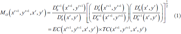
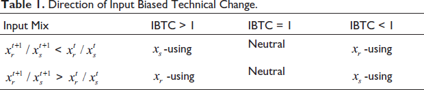
EC will be greater than one if there is an increase in efficiency. There is technological progress (regress) if the value of TC is greater (less) than unity. In practice, technological change is non-neutral in the input-output space at the various input mix points (Margaritis et al., 2007). Hence, technical change can be broken down into BTC and magnitude of technical change (MTC). The bias term can be further decomposed into output-biased technical change (OBTC) and input-biased technical change (IBTC) (Barros & Weber, 2009; Chen & Yu, 2014; Färe & Grosskopf, 1997). That is,

TC= [MTC] × [BTC]

= [MTC] × [OBTC] × [IBTC]

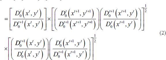
= [\frac{D_{0}^{t} (x^{t}, y^{t})}{D_{0}^{t + 1} (x^{t}, y^{t})}] \times {[(\frac{D_{0}^{t} (x^{t + 1}, y^{t + 1})}{D_{0}^{t + 1} (x^{t + 1}, y^{t + 1})}) (\frac{D_{0}^{t + 1} (x^{t + 1}, y^{t})}{D_{0}^{t} (x^{t + 1}, y^{t})})]}^{\frac{1}{2}} \times {[(\frac{D_{0}^{t + 1} (x^{t}, y^{t})}{D_{0}^{t} (x^{t}, y^{t})}) (\frac{D_{0}^{t} (x^{t + 1}, y^{t})}{D_{0}^{t + 1} (x^{t + 1}, y^{t})})]}^{\frac{1}{2}}

(2)

MTC denotes Hicks-neutral technical change. From Equation (2), if OBTC and IBTC are equal to one, then technical change is Hicks neutral. Conversely, if values of OBTC (or IBTC) are greater than unity, then technical change with bias amplifies growth in TFP, and is the reverse if values of OBTC (or IBTC) are less than one. Since we are interested in looking at the using/saving characteristics of inputs, in this study, TFP has been computed considering single output. This implies that OBTC = 1. Therefore, TC = [MTC] × [IBTC].¹

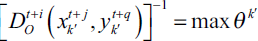
Re-dating the variables and reference technology, six output distance functions in Equation (2) can be computed using the DEA technique under CRS for each country/DMU (k’) as follows:

{[D_{O}^{t + i} (x_{k^{'}}^{t + j}, y_{k^{'}}^{t + q})]}^{- 1} = \max θ^{k^{'}}

subject to

$- θ^{k^{'}} y_{k^{'}, m}^{t + q} + \sum_{k = 1}^{K} z_{k}^{t + i} y_{k, m}^{t + i} \geq 0, m = 1, \dots, M$ (No. of outputs)

$x_{k^{'}, n}^{t + j} - \sum_{k = 1}^{K} z_{k}^{t + i} x_{k, m}^{t + i} \geq 0, n = 1, \dots, N$ (No. of inputs)

$z_{k}^{t + i} \geq 0, k = 1, \dots, K,$ (No. of DMUs)

where ${[D_{O}^{t} (x_{k^{'}}^{t}, y_{k^{'}}^{t})]}^{- 1}$ is calculated with (i, j, q) = (0,0,0), ${[D_{O}^{t + 1} (x_{k^{'}}^{t + 1}, y_{k^{'}}^{t + 1})]}^{- 1}$ with (i, j, q) = (1,1,1), ${[D_{O}^{t} (x_{k^{'}}^{t + 1}, y_{k^{'}}^{t + 1})]}^{- 1}$ with (i, j, q) = (0,1,1), ${[D_{O}^{t + 1} (x_{k^{'}}^{t}, y_{k^{'}}^{t})]}^{- 1}$ with (i, j, q) = (1,0,0), ${[D_{O}^{t} (x_{k^{'}}^{t + 1}, y_{k^{'}}^{t})]}^{- 1}$ with (i, j, q) = (0, 1, 0) and ${[D_{O}^{t + 1} (x_{k^{'}}^{t + 1}, y_{k^{'}}^{t})]}^{- 1}$ with (i, j, q) = (1,1,0). The scalar of the proportional expansion in output for a given input vector is denoted by θ and $z_{k}^{t + i}$ depicts the intensity in which production unit k is employed in production.

There is evidence of neutral or non-neutral technology. While considering the shift in inward or outward technological frontier (as seen previously), the direction in the technical bias moves also becomes important because it helps to interpret whether the input mix of DMU coordinates with that of technical change, which subsequently would affect output and productivity. In this study, IBTC has been considered by utilizing the input distance function, which helps view the idea of bias direction by isoquants in a better way (Chen & Yu, 2014). The input function is a reciprocal of the output function under CRS and, thus, IBTC can be written as follows:

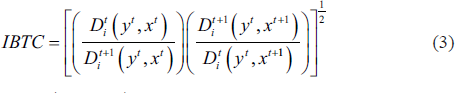
I B T C = {[(\frac{D_{i}^{t} (y^{t}, x^{t})}{D_{i}^{t + 1} (y^{t}, x^{t})}) (\frac{D_{i}^{t + 1} (y^{t}, x^{t + 1})}{D_{i}^{t} (y^{t}, x^{t + 1})})]}^{\frac{1}{2}}

(3)

where $D_{i}^{t} (y^{t}, x^{t})$ = sup{ρ: $(y^{t}, x^{t} / ρ) ϵ L^{t}$ } and the input set L^t = {(y^t, x^t ) : x^t can produce y^t }. If IBTC = 1, then it is a case of Hicks-neutral technical change, and it is non-neutral if IBTC ≠ 1. In the latter case, the direction of bias (Färe et al., 2001) can be shown by following Figure 1.

Figure 1.

Input Biased Technical Change.

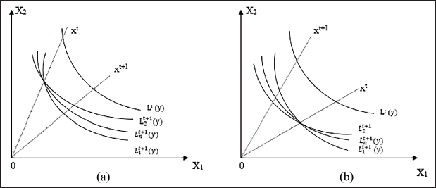
Assuming that technical progress occurs from period t to period t+1, the four input sets in Figure 1 ( $L^{t} (y),$ $L_{2}^{t + 1} (y), L_{n}^{t + 1} (y) a n d L_{1}^{t + 1} (y)$ ) produce y amount of output level. The latter three sets depict different types of technical change. x^t and x^t+1 are the input mix ratios in t and t+1 periods, respectively. Holding the input mix constant, there is Hicks-neutral technical progress if there is constant marginal rate of substitution (MRS) between two inputs, whereas if there is increase (decrease) of MRS between the two inputs, then technical progress is $x_{1}$ -using ( $x_{2}$ -using) (Barros & Weber, 2009; Chen & Yu, 2014). Correspondingly, $L_{n}^{t + 1} (y)$ shows input set with a Hicks-neutral technical change, $L_{1}^{t + 1} (y)$ , with $x_{1}$ -using and $L_{2}^{t + 1} (y)$ with $x_{2}$ -using technical change in time period t+1. The subscripts $1$ and $2$ denote the two inputs $x_{1}$ and $x_{2}$ , respectively.

Borrowing from Färe et al. (1994), it can be shown that different input mix (maybe due to difference in relative factor prices or some development strategy considerations) in two time periods along with the different IBTC values can yield varied direction of BTC results. This is depicted in Table 1 for inputs $r$ and $s$ ( $r$ , $s = 1, \dots, N, r \neq s)$ . When $x_{2}^{t + 1} / x_{1}^{t + 1}$ < $x_{2}^{t} / x_{1}^{t}$ (i.e., x^t+1 < x^t in Figure 1a),   $x_{1}$ -using ( $x_{2}$ -saving) technical change is analogous with IBTC > 1 and $x_{2}$ -using ( $x_{1}$ -saving) technical change corresponds with IBTC < 1. Conversely, $x_{2}$ -using ( $x_{1}$ -saving) technical change go hand-in-hand with IBTC > 1 and there is association of $x_{1}$ -using ( $x_{2}$ -saving) technical change with IBTC < 1 when $x_{2}^{t + 1} / x_{1}^{t + 1}$ > $x_{2}^{t} / x_{1}^{t}$ (i.e., x^t+1 > x^t in Figure 1b) (Barros & Weber, 2009; Färe et al., 2001). Regardless of what the input mix is, neutral technical change occurs if IBTC = 1. In addition, if $x_{2}^{t + 1} / x_{1}^{t + 1}$ = $x_{2}^{t} / x_{1}^{t}$ , then IBTC = 1. However, in this case, one cannot draw any inference about the type of technical change.

Table 1.

Direction of Input Biased Technical Change.

Input Mix	IBTC > 1	IBTC = 1	IBTC < 1
$x_{r}^{t + 1} / x_{s}^{t + 1}$ < $x_{r}^{t} / x_{s}^{t}$	$x_{s}$ -using	Neutral	$x_{r}$ -using
$x_{r}^{t + 1} / x_{s}^{t + 1}$ > $x_{r}^{t} / x_{s}^{t}$	$x_{r}$ -using	Neutral	$x_{s}$ -using

If there is mismatch between direction of technical progress and input mix, a negative bias effect on productivity is realized since cost of resource use would be higher (Chen & Yu, 2014).

Energy Efficiency—DEA Approach

By considering a DMU/country economy $k = 1,2, \dots, K$ as an entity, non-energy input vector $x = (x_{1 k}, x_{2 k}, \dots, x_{N k}) ϵ R_{+}^{N}$ and the scalar energy input $e ϵ R_{+}$ can be transformed into a vector of desirable output $y = (y_{1 k}, y_{2 k}, \dots, y_{M k}) ϵ R_{+}^{M}$ and a vector of undesirable output $z = (z_{1 k}, z_{2 k}, \dots, z_{J k}) ϵ R_{+}^{J}$ under a technology set $Q$ defined as $= \{(x, e; y, z) : x a n d e c a n p r o d u c e y a n d z\}$ (Banker et al., 1984). The technology for the input-oriented efficiency scores can then be represented by its production possibility set $T = {(x ϵ R_{+}^{N}, e ϵ R_{+}) : (x, e; y, z) ϵ Q}$ based on a few regularity assumptions of all observed input-output combinations, free disposability with respect to inputs and outputs, and convexity. In addition, constant returns to scale is assumed, which implies that all radial expansions and (non-negative) contractions of the feasible input-output combinations are feasible. The efficiency analysis under the by-production and joint-production approaches are on the lines of Rakshit and Mandal (2020).

By-Production Approach

Under this approach, energy efficiency estimates have been obtained using the output-oriented directional inefficiency (Ray et al., 2018) as was also computed by Rakshit and Mandal (2020). Following Murty et al. (2012) and Ray et al. (2018), the production possibility set is as follows:

T = \{(x, e; y, z) : (x, e; y) \in T^{y} a n d (e; z) \in T^{z}\} .

For a given input bundle $(x^{0}, e^{0})$ wherein the output set is $P (x^{0}, e^{0})$ , the output-oriented directional (in)efficiency can be represented as $(\vec{D}) (y_{0}, z_{0} | x^{0}, e^{0}) = m a x θ : ((1 + θ) y_{0}, (1 - θ) z_{0}) \in P (x^{0}, e^{0})$ (Rakshit & Mandal, 2020). Under the by-production approach, the objective of the DDF is to reduce the undesirable output and the energy input and to concurrently increase the desirable output to the largest extent possible without increasing non-energy inputs. Here, weakly disposability is assumed between the undesirable output and energy input (Rakshit & Mandal, 2020). The (in)efficiency measurement under CRS technology under DDF is derived by solving the following problem:

Model R

θ^{*} = \max θ

s . t . \sum_{k = 1}^{K} x_{n k} λ_{k} \leq x_{n 0}, n = 1, 2, \dots, N (Non-energy inputs)

(4a)

\sum_{k = 1}^{K} e_{k} λ_{k} = (1 - θ) e_{0} (Energy)

(4b)

\sum_{k = 1}^{K} y_{m k} λ_{k} \geq (1 + θ) y_{m 0}, m = 1, 2, \dots, M (Desirable output)

(4c)

\sum_{k = 1}^{K} z_{j k} λ_{k} = (1 - θ) z_{j 0}, j = 1, 2, \dots, J (Undesirable output)

(4d)

λ_{k} \geq 0, k = 1, 2, \dots, K (DMUs)

(4e)

DMU’s technical inefficiency is indicated by $θ^{*}$ . An efficient DMU operating on the frontier has $θ^{*} = 0$ and $θ^{*} > 0$ for an inefficient DMU. For Model R, technical efficiency (TE) is computed by subtracting the value of $θ^{*}$ from unity (Rakshit & Mandal, 2020).

Joint-Production Approach

Based on the benefit function (Luenberger, 1992) that was propounded by Chambers et al. (1996), good outputs are expanded and bad outputs are simultaneously reduced to the largest extent possible under the DDF following the joint-production approach without increasing energy and non-energy inputs (Rakshit & Mandal, 2020).

The technology set, $S$ , characterized by a convex hull, can be defined as $S = \{(y, e, x, z) : x a n d e c a n p r o d u c e y a n d z\}$ (Banker et al., 1984). It assumes the properties of ‘null-jointness’ between the good and the bad outputs, joint weak disposability between desirable and undesirable outputs, and strong disposability of the desirable output. Projecting the observed bundle $({x_{0}, y}_{0}, z_{0})$ onto the efficient frontier along the desired direction depicted by some reference input-output bundle $(g^{x}, g^{y}, - g^{z})$ , the directional technology distance function can be specified as $(\vec{D}) ({x_{0}, y}_{0}, z_{0} | 0, {y_{0}, - z}_{0}) = m a x θ : ((1 + θ) y_{0}, (1 - θ) z_{0}) \in S$ . The efficiency is measured in a direction portrayed by the direction vector $g = (g^{x}, g^{y}, - g^{z}) = (0, {y_{0}, - z}_{0})$ . Hence, given the technology and the direction vector, DDF evaluates the largest possible expansion of good output and contraction of bad output (Mandal & Madheswaran, 2010; Rakshit & Mandal, 2020). The DEA problem for the DDF is shown as follows:

Model C

θ^{*} = \max θ

s . t . \sum_{k = 1}^{K} x_{n k} λ_{k} \leq x_{n 0}, n = 1, 2, \dots, N (Energy and non-energy inputs)

(5a)

\sum_{k = 1}^{K} y_{m k} λ_{k} \geq (1 + θ) y_{m 0}, m = 1, 2, \dots, M (Desirable outputs)

(5b)

\sum_{k = 1}^{K} z_{j k} λ_{k} = (1 - θ) z_{j 0}, j = 1, 2, \dots, J (Undesirable outputs)

(5c)

λ_{k} \geq 0, k = 1, 2, \dots, K (DMUs

(5d)

Following Rakshit and Mandal (2020), the value of $θ^{*}$ represents technical inefficiency of the DMU. An efficient DMU that operates on the frontier will have $θ^{*} = 0$ , and $θ^{*} > 0$ for an inefficient DMU. TE from Model C can be computed by subtracting the value of $θ^{*}$ from 1. Constraints (5b) and (5c) show strong disposability of good output and weak disposability of bad output, respectively.

Since in Model C the energy input is not scaled down by a factor of $(1 - θ)$ as is carried out under Model R, the energy efficiency estimated from these two models may not be strictly comparable. Hence, an alternative would be to measure efficiency by considering the reduction in energy intensity. This is known as energy intensity efficiency (Mukherjee, 2010). From Model R, this efficiency can be computed as $\frac{\frac{e^{*}}{y^{*}}}{\frac{e^{0}}{y^{0}}} = \frac{(1 - θ^{*})}{(1 + θ^{*})}$ and the corresponding efficiency from Model C can be calculated as $\frac{\frac{e^{*}}{y^{*}}}{\frac{e^{0}}{y^{0}}} = \frac{1}{(1 + θ^{*})}$ .

Data Descriptions

In the present study, the sample data comprises of 149 economies that have been further grouped into low-income, middle-income and high-income economies² over the time period 1993–2013. The aggregate measures of output used in the analysis are gross domestic output (GDP) in million US$ in 2011 PPP and carbon dioxide emissions (CO₂) in million tonnes. Labour (in millions), capital (million 2011 US$) and energy (million metric tonnes of oil equivalent [Mtoe]) have been regarded as inputs in the analysis. Following along the lines of Rakshit and Mandal (2020), energy has been considered in the form of primary energy.³ This takes into account coal, petroleum, dry natural gas excluding supplemental gaseous fuels, nuclear energy, conventional hydroelectricity, geothermal energy, solar energy, wind energy, wood and wood-derived fuels, biomass waste, fuel ethanol and biodiesel, respectively. Data on GDP, labour and capital have been extracted from Penn World Table (PWT 9.0),⁴ energy from the U.S. Energy Information Administration and CO₂ from World Development Indicators. Since the data are at the country level, CRS technology is assumed (Ray et al., 2018). Table 2 depicts the descriptive statistics of the data. It can be discerned that there is substantial variation in variables across countries and time (Rakshit & Mandal, 2020).

Table 2.

Descriptive Statistics of the Data Variables (1993–2013).

	Labour (in Million Persons)	Capital  (in Million 2011 US$)	Energy  (in Million Mtoe)	GDP  (in Million 2011 US$ PPP)	CO₂  (in Million Tonnes)
Global
Mean	17.97	1,576,740	70.85	434,897.30	995.76
SD	71.25	4,788,226	260.28	1,444,741	5,314.46
Max	793.02	60,900,000	2,991.93	16,200,000	102,580.10
Min	0.03	919.15	0.03	155.72	0.33
Low-income
Mean	6.04	50,737.21	0.94	17,591.99	19.40
SD	6.85	63,136.48	1.07	18,628.57	26.89
Max	43.68	473,003.60	5.90	130,283.40	177.96
Min	0.11	1,976.57	0.03	293.22	0.70
Middle-income
Mean	24.56	1,139,897	57.93	330,848.20	1631.74
SD	93.37	3,726,017	216.02	1,088,932	7030.56
Max	793.02	60,900,000	2,991.93	15,900,000	102,580.10
Min	0.03	919.15	0.03	155.72	0.33
High-income
Mean	12.05	3,475,092	143.11	922,047.60	310.74
SD	24.02	7,150,524	383.32	2,224,015	860.08
Max	148.20	50,600,000	2,549.28	16,200,000	5,789.73
Min	0.14	15,676.92	0.83	5,318.82	2.06

The correlation matrix of the inputs and outputs is presented in Table 3. Significantly positive correlation coefficients imply that output values also go up when inputs are increased. This makes energy efficiency analysis feasible (Zhang & Choi, 2013).

Table 3.

Correlation Matrices for Inputs and Outputs (1993–2013).

	Labour	Capital	Energy	GDP	CO₂
Labour	1.000
Capital	0.603*	1.000
Energy	0.636*	0.942*	1.000
GDP	0.620*	0.984*	0.971*	1.000
CO₂	0.860*	0.582*	0.665*	0.591*	1.000

*Significance at the 5% level.

Results and Discussion

Total Factor Productivity and Its Decomposition

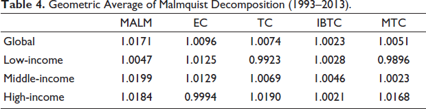
Using the approach described in Section 3, we first compute the MALM and its decompositions for economies at the global level as well as for low-, middle- and high-income economies in every adjacent pair of years and then calculate the geometric average of the same. The results are reported in Table 4. TFP had shown an improvement in the case of all the sample observations. It can be observed that from 1993 to 2013, TFP increased by 1.71% at the global level. It increased by 0.47%, 1.99% and 1.84% for low-, middle- and high-income economies, respectively. At the global level, this improvement has been contributed by both TE change (0.96%) and technical change (0.74%). In low-income economies, the increase in TFP was due to progress in TE (value of 1.0125). However, technical change experienced regress (value of 0.9923) in low-income economies. Middle-income economies witnessed an improvement in TFP (1.99%) due to progress in TE (1.29%) as well as in technical change (0.69%). TFP increased in high-income economies by 1.84%. This improvement in productivity can be attributed to progress in technical change (value of 1.0190). But there was TE regress (value of 0.9994) from 1993 to 2013 in high-income economies. Table 4 also shows that the average IBTC index equals 1.0023, 1.0028, 1.0046 and 1.0021 for the global, low-, middle- and high-income economies. The value of the IBTC index being very close to one reflects that there have been relatively smaller biased technical changes. In addition, except for low-income economies, other groups of economies have displayed neutral technology progress over the period, as observed from the MTC values.

Table 4.

Geometric Average of Malmquist Decomposition (1993–2013).

	MALM	EC	TC	IBTC	MTC
Global	1.0171	1.0096	1.0074	1.0023	1.0051
Low-income	1.0047	1.0125	0.9923	1.0028	0.9896
Middle-income	1.0199	1.0129	1.0069	1.0046	1.0023
High-income	1.0184	0.9994	1.0190	1.0021	1.0168

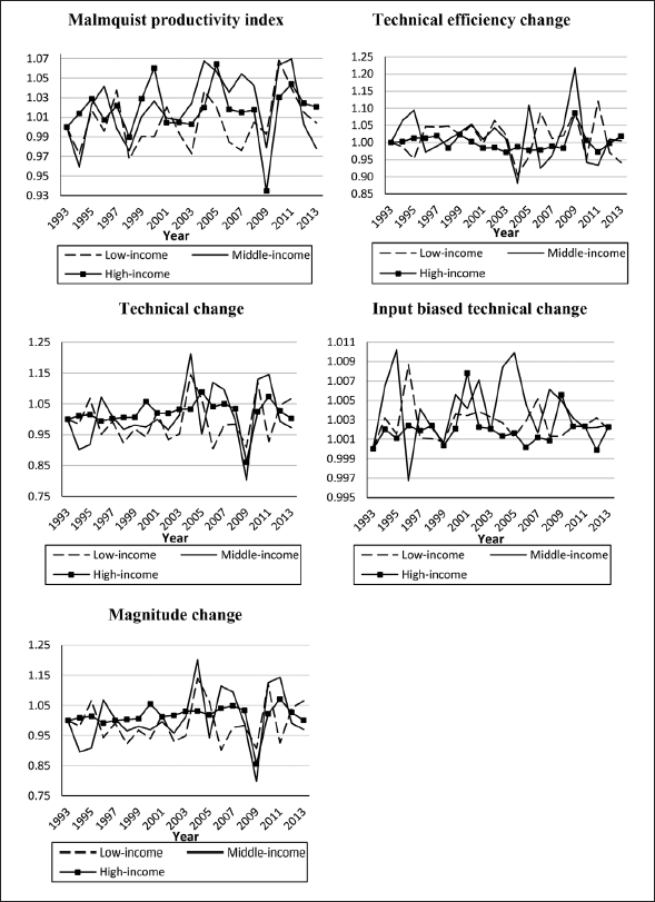
The variations in productivity among different income groups of economies have been further examined. The evolution of change in TFP and its decompositions for low-, middle- and high-income economies during the study period are presented in Figure 2. The three groups of economies seem to display an increasing, albeit fluctuating, trend in TFP change over the years. This fluctuation in TFP change is more pronounced for high-income economies, followed by middle-income economies and then by low-income economies. It implies that the rise and fall of productivity in high-income economies have been relatively more distinct compared to in middle and low-income economies over the years. The trend of technical change follows the trend of productivity change for all the economies, suggesting that the progress and regress in technical change is reflected in the corresponding increase and decrease in TFP. This implies that technical innovation is crucial for improving TFP for all the economies. The TE change, in contrast, exhibits a trend opposite of that seen under TFP change for all the economies. It can be inferred that more efficient production is necessary to complement the growth in productivity.

Figure 2.

Productivity and Its Decomposition for Different Income Groups of Economies.

Total Factor Productivity, Technical Change and Energy Efficiency at the Global Level

Table 5 reports the annual index of both models of energy efficiency scores as well as productivity index and its decompositions. The average energy efficiency based on the DDF model considering the reduction in polluting input (energy) and undesirable output and the proportionate increase in the desirable output (Model R) is found to be substantially lower than that obtained from the model considering only the contraction in undesirable output along with simultaneous expansion in the desirable output (Model C). This is because Model R involves an added restriction and therefore leads to a lower value of the objective function in the maximization problem. The Wilcoxon Rank-Sum test has been employed⁵ to verify whether adding the restriction in the efficiency model results in significantly different estimates of energy efficiency. Since the value of two-tailed ‘p’ statistic is found to be less than 0.0005, the null hypothesis can be rejected at 1% level, implying that the additional constraint considered in Model R results in significantly different energy efficiency estimates. As also observed by Rakshit and Mandal (2020), over the time period 1993–2013, there was improvement in energy efficiency, except in 1994, 1998 and 2009 when it witnessed a marginal dip that coincided with the Mexican peso crisis, the Asian financial crisis and the 2008 recession, respectively. In these years, oil prices also fell.⁶ Overall, there has been efficient usage of energy when there has been rise in oil prices. This demonstrates that induced innovation hypothesis has been important at the global level in the short run.

Table 5.

Measures of Productivity Index and Energy Efficiency at the Global Level.

	Energy Efficiency		Productivity
Year^a	Model R	Model C	MALM	EC	TC	IBTC	MTC	Crude Oil Price^b
1993	0.254	0.613	1.0000	1.0000	1.0000	1.0000	1.0000	18.43
1994	0.248	0.610	0.9755	1.0356	0.9420	1.0030	0.9392	17.20
1995	0.249	0.611	1.0185	1.0671	0.9545	1.0021	0.9525	18.43
1996	0.255	0.613	1.0238	1.0189	1.0048	1.0018	1.0027	22.12
1997	0.262	0.612	1.0124	0.9955	1.0169	1.0015	1.0155	20.61
1998	0.254	0.608	0.9801	1.0133	0.9673	1.0013	0.9661	14.42
1999	0.260	0.608	1.0115	1.0218	0.9898	1.0008	0.9891	19.34
2000	0.273	0.613	1.0280	1.0398	0.9887	1.0018	0.9870	30.38
2001	0.278	0.614	1.0121	0.9864	1.0260	1.0037	1.0222	25.98
2002	0.281	0.612	1.0031	1.0494	0.9559	1.0046	0.9516	26.18
2003	0.284	0.612	1.0081	0.9885	1.0198	1.0015	1.0183	31.08
2004	0.301	0.620	1.0523	0.8627	1.2197	1.0040	1.2149	41.51
2005	0.327	0.633	1.0541	1.0519	1.0021	1.0041	0.9980	56.64
2006	0.340	0.639	1.0221	0.9654	1.0587	1.0018	1.0568	66.05
2007	0.362	0.650	1.0367	0.9850	1.0525	1.0016	1.0508	72.34
2008	0.384	0.660	1.0312	1.0235	1.0075	1.0017	1.0058	99.67
2009	0.371	0.648	0.9688	1.1875	0.8158	1.0048	0.8119	61.95
2010	0.400	0.663	1.0533	0.9606	1.0965	1.0012	1.0952	79.47
2011	0.436	0.686	1.0572	0.9577	1.1039	1.0015	1.1023	94.88
2012	0.447	0.692	1.0105	1.0079	1.0027	1.0013	1.0014	94.05
2013	0.447	0.693	0.9887	1.0087	0.9802	1.0014	0.9789	97.98

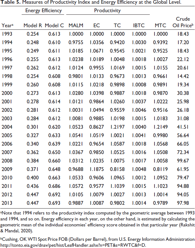
^aNote that 1994 refers to the productivity index computed by the geometric average between 1993 and 1994, and so on. Energy efficiency in each year, on the other hand, is estimated by calculating the geometric mean of the individual economies’ efficiency score obtained in that particular year (Rakshit & Mandal, 2020).

^bCushing, OK WTI Spot Price FOB (Dollars per Barrel), from U.S. Energy Information Administration http://tonto.eia.gov/dnav/pet/hist/LeafHandler.ashx?n=PET&s=RWTC&f=D.

A similar increase in trend was also be observed in the MALM. This can be discerned by the fact that the values of MALM are all greater than one except in 1994, 1998, 2009 and 2013. By observing the trends in the components of MALM over the years, it appears that both technical change and TE change have been important in driving TFP growth. Hence, innovation advancement as well as increase in the efficiency in production activities have played an important role in raising the TFP at the global level. As mentioned earlier, there has been neutral technical progress over the years. Further, the IBTC values being near one reflects the fact that there is almost consistency with Hicks neutrality on an average over the sample period.

Direction of Technical Change and Energy Efficiency in the Short-Run

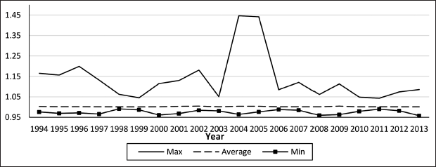
At the global level, countries have experienced a great level of technical bias, as observed in Figure 3. Hence, it becomes imperative to determine the input bias index and direction of technical change for each country. For this purpose, Table 6 summarizes the number of countries having a bias in using relative inputs along with classifying countries on the basis of three IBTC values, namely, >1, <1 and =1, at the global level. In most of the years (16 out of 20), the direction of technology bias matched with the input mix used, denoted by IBTC > 1, at the global level. This has aided in magnifying TFP growth and, subsequently, the GDP of these countries over the years. There are also countries where IBTC < 1, implying that adoption of technology has not coordinated with their input mix (factor markets). There are very few economies that have experienced neutral technical change.

Figure 3.

Maximum and Minimum of IBTC Values at the Global Level.

Table 6.

Distributions of Annual Input Biased Technological Change at the Global Level.

	IBTC			E vs. L			E vs. K			Energy Efficiency
Years	>1	<1	1	E-Using	E-Saving	Neutral	E-Using	E-Saving	Neutral	Model R	Model C
1994	82	65	2	76	71	2	74	73	2	0.254	0.613
1995	75	70	4	84	61	4	72	73	4	0.248	0.610
1996	71	77	1	73	75	1	85	63	1	0.249	0.611
1997	88	60	1	50	98	1	45	103	1	0.255	0.613
1998	87	61	1	83	65	1	88	60	1	0.262	0.612
1999	76	72	1	69	79	1	57	91	1	0.254	0.608
2000	83	64	2	93	54	2	73	74	2	0.260	0.608
2001	89	58	2	45	102	2	34	113	2	0.273	0.613
2002	93	53	3	68	78	3	66	80	3	0.278	0.614
2003	92	57	0	88	61	0	85	64	0	0.281	0.612
2004	76	73	0	59	90	0	68	81	0	0.284	0.612
2005	79	70	0	87	62	0	77	72	0	0.301	0.620
2006	69	79	1	80	68	1	90	58	1	0.327	0.633
2007	80	67	2	69	78	2	85	62	2	0.34	0.639
2008	77	70	2	87	60	2	72	75	2	0.362	0.650
2009	102	46	1	53	95	1	54	94	1	0.384	0.660
2010	72	75	2	65	82	2	72	75	2	0.371	0.648
2011	76	71	2	88	59	2	80	67	2	0.400	0.663
2012	66	79	4	79	66	4	78	67	4	0.436	0.686
2013	79	69	1	48	100	1	51	97	1	0.447	0.692

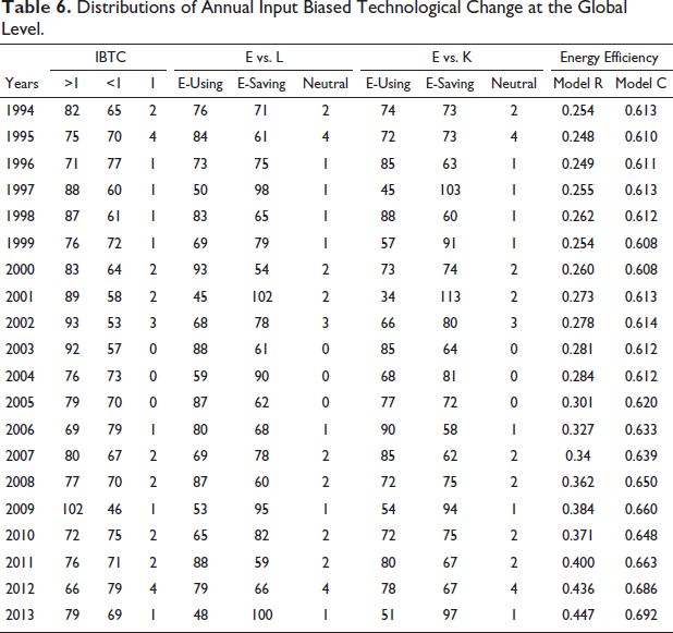
With three inputs, capital (K), labour (L) and energy use (E), two situations have been examined in this study to identify the direction of technological bias: E vs. L and E vs. K, presented in Table 5. Looking at the pairs of E vs. L and E vs. K, in almost half of the time period under consideration, the economies had E-saving (or L- and K-using) bias. It can be observed that during the years of the economic downturn (1999 and 2009–2010), when there was also a fall in energy efficiency, the economies went for E-saving (or L- and K-using) bias. It meant that energy-saving technology was adopted in these years to fuel the economic growth to keep the momentum of energy-efficiency improvement in place. This may be explained by the fact that during periods of economic instability, economies prefer to use domestic inputs rather than heavily rely on imported energy resulting in biased technical change (Binswanger, 1974). However, energy may still be consumed in using other inputs in the production process (embodied energy), leading to a marginal fall in energy efficiency.

Direction of Technical Change and Energy Efficiency in the Long-Run

Table 7 displays the distribution of IBTC and change in energy efficiency over the period 1993–2013 at the global level. The difference between Table 6 and Table 7 is that earlier the MALM for a given unit was compared at two different years by constructing a chain-link of adjacent productivity indexes cumulatively. However, there is also a need to determine the MALM and its components over the entire period as well as for each country since the chain version for panel data is not transitive (Barros & Weber, 2009; Chen & Yu, 2014). Through such a procedure, we can check whether, similar to short-run results, countries underwent neutral technical change in the long-run as well or not. Table 7 shows that in none of the situations (E vs. L and E vs. K), neutral technical change was experienced in the long run. These findings show that the extent of the bias is more visible over a longer period where its direction matched the input mix and technological advancement occurred due to series of dynamic evolutions. Most of the economies (68.46% countries of the total global sample) had IBTC > 1, implying that biased technical change magnified TFP growth over time. The bias is more towards E-using/L-saving in E vs. L situations (44.97% countries). These economies, in essence, went for energy-using technology and used relatively less labour than energy, leading to a relatively lesser increase in energy efficiency (2.50% and 0.52% under Model R and Model C, respectively) as compared to when economies went for energy-saving technology (3.20% and 0.90% under Model R and Model C respectively). Under the case of E vs. K, 51.68% of the economies at the global level had a technological bias towards E-saving/K-using technology. The use of relatively more energy than that of capital under E vs. K meant that the energy-efficiency improvement was more pronounced (3.05% under Model R and 0.76% under Model C) than when the economies used comparatively less energy vis-à-vis capital (1.73% under Model R and 0.33% under Model C).

Table 7.

Distribution of Input Biased Technical Change and Change in Energy Efficiency (%) at the Global Level: 1993–2013.

	E vs. L		E vs. K
	${(\frac{E}{L})}_{2013} > ({\frac{E}{L})}_{1993}$	${(\frac{E}{L})}_{2013} < ({\frac{E}{L})}_{1993}$	${(\frac{E}{K})}_{2013} > ({\frac{E}{K})}_{1993}$	${(\frac{E}{K})}_{2013} < ({\frac{E}{K})}_{1993}$
IBTC > 1	E-using (67)	E-saving (35)	E-using (25)	E-saving (77)
Model R	2.50	3.20	1.73	3.05
Model C	0.52	0.90	0.33	0.76
IBTC < 1	E-saving (22)	E-using (25)	E-saving (26)	E-using (21)
Model R	2.62	4.16	2.01	5.19
Model C	0.42	0.69	0.30	0.90
IBTC = 1	Neutral (0)	Neutral (0)	Neutral (0)	Neutral (0)

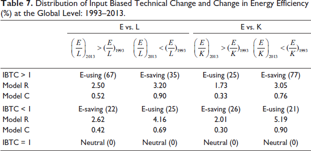
Focussing on the technology bias results of countries with IBTC < 1 from Table 7, it is observed that 16.78% of the economies showed E-using/L-saving bias (when E vs. L) in 1993–2013. These economies took up E-using technology but used comparatively less energy, experiencing an improvement of energy efficiency (4.16% and 0.69% under Model R and Model C, respectively) on the one hand but shrinking of TFP growth (since IBTC < 1) on the other hand. In E vs. K situations, most of the economies (17.45% countries of the global sample) went for E-saving/K-using technology but used relatively more energy than capital, leading to dampening of energy-efficiency improvement accompanied by the fall in TFP growth. This may be expounded by the fact that these economies might have a relatively abundant endowment of labour, and such a technological innovation would make them more productive. But in this process, the wages of these skilled workers start going up, making the producers to use relatively more energy than labour leading to a reduction in energy-efficiency improvement and increase in unemployment in these economies.

To better understand the direction of technical change, its coordination with input mix and its association with energy efficiency at the global level, this study further investigates these dynamics for each income group of economies.

Total Factor Productivity, Technical Change and Energy Efficiency for Low, Middle and High-Income Economies

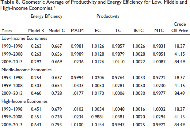
Table 8 exhibits the annual index of both models of energy-efficiency scores as well as productivity index and its decompositions for the low-, middle- and high-income economies in different sub-periods. Similar to the findings at the global level, the average energy efficiency under Model R is substantially lower than that obtained under Model C. From the Wilcoxon Rank-Sum test, it can be observed that the added restriction in Model R results in significantly different energy efficiency estimates. The energy efficiency in low-income economies have been low and have fluctuated over the years (Rakshit & Mandal, 2020). It is because these economies may not be utilizing the most advanced technologies in their energy-intensive sectors that comprise basic metals, non-metallic minerals, paper and paper products, coke, petroleum refining and so on. Their lower energy efficiencies can also be attributed to their dependence on low-quality fuels. 50%–80% of total primary energy use is constituted by traditional biomass in 75% of low-income economies comprising least developed countries (LDCs) as of 2014. In the remaining LDCs, oil products contribute a major share in total primary energy use. However, there is utilization of natural gas, coal and renewable energy (hydroelectricity in Malawi and Mozambique) in few LDCs (UNCTAD, 2017). Since relatively fewer low-income economies use oil hence, it can be observed from Table 9 that the trend in energy efficiency does not entirely correspond with the trend in oil prices. Thus, it may be inferred that change in oil prices may not have much bearing on low-income economies’ energy efficiency.

Table 8.

Geometric Average of Productivity and Energy Efficiency for Low, Middle and High-Income Economies.⁷

	Energy Efficiency		Productivity
Years	Model R	Model C	MALM	EC	TC	IBTC	MTC	Crude Oil Price
Low-Income Economies
1993–1998	0.263	0.667	0.9981	1.0126	0.9857	1.0026	0.9831	18.37
1999–2008	0.263	0.656	0.9989	1.0128	0.9879	1.0028	0.9851	41.15
2009–2013	0.292	0.669	1.0236	1.0126	1.0110	1.0022	1.0087	84.49
Middle-Income Economies
1993–1998	0.254	0.637	0.9994	1.0206	0.9764	1.0033	0.9722	18.37
1999–2008	0.303	0.654	1.0333	1.0050	1.0281	1.0050	1.0230	41.15
2009–2013	0.460	0.728	1.0177	1.0170	1.0006	1.0030	0.9977	84.49
High-Income Economies
1993–1998	0.451	0.679	1.0102	1.0054	1.0048	1.0016	1.0032	18.37
1999–2008	0.551	0.738	1.0234	0.9881	1.0381	1.0020	1.0294	41.15
2009–2013	0.643	0.793	1.0100	1.0154	0.9947	1.0025	0.9922	84.49

Table 9.

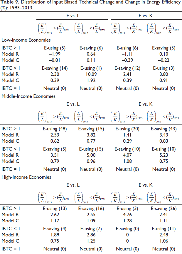
Distribution of Input Biased Technical Change and Change in Energy Efficiency (%): 1993–2013.

	E vs. L		E vs. K
	${(\frac{E}{L})}_{2013} > ({\frac{E}{L})}_{1993}$	${(\frac{E}{L})}_{2013} < ({\frac{E}{L})}_{1993}$	${(\frac{E}{K})}_{2013} > ({\frac{E}{K})}_{1993}$	${(\frac{E}{K})}_{2013} < ({\frac{E}{K})}_{1993}$
Low-Income Economies
IBTC > 1	E-using (5)	E-saving (6)	E-using (6)	E-saving (5)
Model R	–1.99	0.64	–1.11	0.10
Model C	–0.81	0.11	–0.39	–0.22
IBTC < 1	E-saving (14)	E-using (1)	E-saving (12)	E-using (3)
Model R	2.30	10.09	2.41	3.80
Model C	0.39	1.92	0.39	0.91
IBTC = 1	Neutral (0)	Neutral (0)	Neutral (0)	Neutral (0)
Middle-Income Economies
	E vs. L		E vs. K
	${(\frac{E}{L})}_{2013} > ({\frac{E}{L})}_{1993}$	${(\frac{E}{L})}_{2013} < ({\frac{E}{L})}_{1993}$	${(\frac{E}{K})}_{2013} > ({\frac{E}{K})}_{1993}$	${(\frac{E}{K})}_{2013} < ({\frac{E}{K})}_{1993}$
IBTC > 1	E-using (48)	E-saving (15)	E-using (20)	E-saving (43)
Model R	2.53	3.82	1.41	3.43
Model C	0.62	0.77	0.29	0.83
IBTC < 1	E-saving (5)	E-using (15)	E-saving (10)	E-using (10)
Model R	3.51	5.00	4.07	5.23
Model C	0.79	0.96	1.08	0.75
IBTC = 1	Neutral (0)	Neutral (0)	Neutral (0)	Neutral (0)
High-Income Economies
	E vs. L		E vs. K
	${(\frac{E}{L})}_{2013} > ({\frac{E}{L})}_{1993}$	${(\frac{E}{L})}_{2013} < ({\frac{E}{L})}_{1993}$	${(\frac{E}{K})}_{2013} > ({\frac{E}{K})}_{1993}$	${(\frac{E}{K})}_{2013} < ({\frac{E}{K})}_{1993}$
IBTC > 1	E-using (13)	E-saving (16)	E-using (3)	E-saving (26)
Model R	2.62	2.55	4.76	2.41
Model C	1.17	1.09	1.28	1.11
IBTC < 1	E-saving (4)	E-using (7)	E-saving (0)	E-using (11)
Model R	1.89	2.86	0	2.48
Model C	0.75	1.25	0	1.06
IBTC = 1	Neutral (0)	Neutral (0)	Neutral (0)	Neutral (0)

As also observed at the global level, middle-income economies’ energy efficiency trend follows a similar pattern. It improved over the period 1993–2013, except in 1994, 1998 and 2009, coinciding with the Mexican peso crisis, the Asian financial crisis and the 2008 recession, respectively. Since the turn of the century, there has been an improvement in energy-efficiency levels in the middle-income economies that can be contributed to energy-efficiency advancements in the industrial sector, especially after 2010 (Rakshit & Mandal, 2020). 39% of the global savings in the upper-middle-income economies were due to industrial energy-intensity improvement during 2010–2015. In the same time period, lower-middle-income economies also experienced improvement in industrial energy intensity (International Energy Agency et al., 2018). During the years of economic downturn, the oil prices had also gone down. For instance, in the later quarter of 2008, the slowdown in economic activity led to fall in oil prices from US$ 99.67/barrel to US$ 61.95/barrel in 2009, rendering the use of energy less efficient. However, the rise in oil prices contributed to efficient usage of energy, highlighting the important role played by induced innovation hypothesis in middle-income economies (Rakshit & Mandal, 2020).

There has been improvement in energy efficiency in high-income economies over the period 1993–2013, except in 2009 when it experienced a drastic decline and coincided with the 2008 recession (Rakshit & Mandal, 2020). The development of renewable energy power generation capacity and a consistent decline in energy demand after 2008–2009 have contributed to improvements in energy efficiency in high-income economies.

Similar to energy efficiency, the fluctuating trend was also observed in the MALM in low-income economies. By observing the trends in the components of MALM over the years, it appears that the TE change has been more important in driving TFP growth than the technical change. Hence, policies in low-income economies may be directed towards advancements in innovation in order to spur TFP growth. In addition, there has been neutral technical progress over the years. Further, the IBTC values being near 1 reflects the fact that there is almost consistency with Hicks neutrality on an average over the sample period. An increase in trend was observed in the MALM in middle-income economies. Moreover, the increase in the efficiency in production activities has played an important role in raising the TFP for middle-income economies. The IBTC values being near 1 for most of the years reflects the fact that there is almost consistency with Hicks neutrality on an average over the sample period. The trend in the MALM of high-income economies reveals that there has been productivity growth in all the years except 1998 and 2009. By observing the trends in the components of MALM over the years, it appears that technical change was vital in facilitating TFP growth. Hence, an increase in the technological innovation have played an important role in raising the TFP for high-income economies.

Tables 9 displays the distribution of IBTC and change in energy efficiency over the period 1993–2013 for the low-, middle- and high-income economies. Table 9 shows that in none of the situations (E vs. L and E vs. K), neutral technical change was experienced. Most of the low-income economies (15 out of 26) had IBTC < 1, implying that biased technical change hindered TFP growth over time. This finding is contrary to what was observed in the short run when the direction of technology bias matched with the input mix used in most of the years. In the long run, the technological bias is more towards E-saving (or L- and K-using) in E vs. L (53.84% of the countries from the low-income economies’ sample) and E vs. K (46.15% countries) situations. In essence, these economies went for energy-saving technology and used relatively less labour and capital than energy. This implies that low-income economies have not fully utilized their resource endowments to the maximum potential. This is because of the mismatch between factor endowment and the technologies available in these economies. This has led to energy efficiency improving at a slower rate. This can be discerned from Table 9 when the change in energy efficiency for economies that underwent E-saving technical bias under Model R and Model C has been 2.30% and 0.39% in E vs. L case and 2.41% and 0.39% in E vs. K case, respectively. Focussing on the technology bias results of countries with IBTC > 1 from Table 9, it is observed that 23.08% of the low-income economies showed E-saving/L-using bias (when E vs. L) in 1993–2013. These economies took up E-saving technology and utilized relatively more labour than energy, resulting in energy-efficiency improvements over time. However, when the economies took up E-using technology, there was a decline in energy-efficiency improvement. In the E vs. K situation, most of the economies went for E-using/K-saving technology (23.08% of the countries from the sample of low-income economies) and used relatively more energy than capital. However, these economies witnessed dampening in energy-efficiency improvement as represented by the negative energy efficiency change seen in Table 9.

Most of the middle-income economies (63 out of 83) had IBTC > 1, implying that biased technical change augmented TFP growth over time. In the long run, the technological bias is more towards E-using/L-saving when E vs. L situation (57.83% countries from the sample of middle-income economies) is considered. This brings out the importance of energy as a critical input in the production processes in middle-income economies. However, the utilization of relatively less labour than energy resulted in unemployment in these economies. Looking at the combination of E vs. K, it is observed that 51.81% of economies had a bias towards E-saving/K-using technology in the short- and long-run. Their corresponding energy-efficiency improvement has been 3.43% and 0.83% under Model R and Model C, respectively. The technology bias results of countries with IBTC < 1 from Table 9 also reveals that most of the economies (18.07% countries from the middle-income economies’ sample) showed E-using/L-saving bias (when E vs. L) in 1993–2013 and experienced increase in energy efficiency (5.00% and 0.96% under Model R and Model C, respectively). However, when the economies took up E-saving technology but utilized relatively more energy than labour, energy efficiency increased by only 3.51% and 0.79% under Model R and Model C, respectively, from 1993 to 2013. As under the E vs. L situation, similar observations can also be noticed for the E vs. K pair.

Like the middle-income economies, most of the high-income economies (29 out of 40) had IBTC > 1. In the long run; the technological bias is more towards E-saving (or L- and K-using) when E vs. L (40% countries from the sample of high-income economies), and E vs. K (65% countries from the high-income economies’ sample) situations are considered. Under the outcomes of both E-using and E-saving technical change, high-income economies have had positive energy efficiency advancements over the years. However, from Table 9, it can be observed that economies that went for E-using technology had higher energy-efficiency improvements than those economies that went for E-saving technology. This may be explained by the fact that high-income economies are technology innovators and can develop technologies appropriate for their factor endowment. The technology bias results of countries with IBTC < 1 reveals that most of the economies showed E-using (or L- and K-saving) bias (when E vs. L and E vs. K) in 1993–2013 accompanied by greater increase in energy efficiency. However, when the economies took up E-saving technology but utilized relatively more energy than labour, energy efficiency increased only by 1.89% and 0.75% under Model R and Model C, respectively, from 1993 to 2013.

Conclusion

This paper examines the direction of technical change, its coordination with input mix and its association with energy efficiency at the global level as well as for different income groups of economies (low, middle and high) over the period 1993–2013 using DEA-based MALM and energy efficiency models. The findings reveal that, in most of the years, the bias in the direction of technical change coordinated with the input mix for all the groups of economies in the short-run thereby magnifying TFP growth. This is also observed in the long-run, with the exception of many low-income economies where the direction of technical change did not coordinate with the input mix. This implies that although low-income economies introduce the technology that adapts to their factor markets, these economies are unable to promote the provision of inputs that can make use of the technology they adopt (Chen & Yu, 2014). Since unskilled labour is abundant in these economies, appropriate policies should be formulated to enhance human capital formation and developing their skill so that they adopt to advanced technologies (UNCTAD, 2014).

With respect to labour and capital, except for low-income economies, the rest of the sample of economies’ energy-saving technical change has a positive association with energy-efficiency improvements implying that energy-saving innovation is consistent with achieving higher energy efficiency over time. This reinforces the fact that in low-income economies, the labour as an input in the production processes may not be possessing the required skill and knowledge of the latest technology to carry out improvements in energy efficiency optimally. In middle-income economies, energy-efficiency improvement occurred at the cost of using other inputs, leading to the displacement of labour and unemployment. This can be overcome by efficiently utilizing available resources through the provision of employment opportunities and fostering capital accumulation in different sectors of the economy. The results of this study also suggest that there is substitution of input use between capital, labour and energy and change in technical bias direction due to change in oil prices in different groups of economies.

In this study, it was also observed that there are a considerable number of countries in each group of economies that have a mismatch of technical bias direction, input mix and corresponding advancements in energy efficiency, indicating the need to adjust the direction of research in technologies or to provide an environment in factor market appropriate for these countries in accordance with the structural characteristics of the individual economy. This will aid in improving their productivities as well as energy efficiency.

One important limitation of this analysis is that it does not consider undesirable output, which may lead to biased results in estimating technical change and its direction. A possible area of research in this regard may be to compute BTC by considering both desirable and undesirable outputs. Another possible area of research may be to explore detailed linkages between technology, energy efficiency and productivity by considering different energy inputs at micro and macro levels.

Footnotes

Declaration of Conflicting Interests

The authors declared no potential conflicts of interest with respect to the research, authorship and/or publication of this article.

Funding

The authors received no financial support for the research, authorship and/or publication of this article.

Notes

ORCID iD

Sabuj Kumar Mandal

References

Acemoglu

, & Zilibotti

(2001). Productivity differences. Quarterly Journal of Economics , 116(2), 563–606.

Adesokan

M. B.

(2008). Global productivity growth from 1980–2000: A regional view using the Malmquist total factor productivity index. International Journal of Business and Management , 10(4), 374–390.

Ahmed

E. M.

, & Krishnasamy

(2013). Human capital investment to achieve knowledge-based economy in ASEAN5: DEA applications. Journal of the Knowledge Economy , 4(4), 331–342.

Álvarez-Ayuso

, Delgado-Rodríguez

M. J.

, & Salinas-Jiménez

M. D. M.

(2011). Explaining TFP growth in the European Union at the sector level. Journal of Economic Policy Reform , 14(3), 189–199.

Apergis

, Aye

G. C.

, Barros

C. P.

, Gupta

, & Wanke

(2015). Energy efficiency of selected OECD countries: A slacks based model with undesirable outputs. Energy Economics , 51, 45–53.

Azadeh

, Amalnick

M. S.

, Ghaderi

S. F.

, & Asadzadeh

S. M.

(2007). An integrated DEA PCA numerical taxonomy approach for energy efficiency assessment and consumption optimization in energy intensive manufacturing sectors. Energy Policy , 35(7), 3792–3806.

Banker

R. D.

, Charnes

, & Cooper

W. W.

(1984). Some models for estimating technical and scale inefficiencies in data envelopment analysis. Management Science , 30(9), 1078–1092.

Barros

C. P.

, & Weber

W. L.

(2009). Productivity growth and biased technological change in UK airports. Transportation Research Part E: Logistics and Transportation Review , 45(4), 642–653.

Berndt

E. R.

(1990). Energy use, technical progress and productivity growth: A survey of economic issues. Journal of Productivity Analysis, 2(1), 67–83.

10.

Binswanger

H. P.

(1974). The measurement of technical change biases with many factors of production. American Economic Review , 64(6), 964–976.

11.

Brock

W. A.

, & Taylor

M. S.

(2005). Economic growth and the environment: A review of theory and empirics. In S. Durlauf & P. Aghion (Eds), Handbook of economic growth (Vol. 1, pp. 1749–1821). Elsevier.

12.

Chambers

R. G.

, Chung

, & Färe

(1996). Benefit and distance functions. Journal of Economic Theory , 70(2), 407–419.

13.

Chang

C. C.

, & Luh

Y. H.

(1999). Efficiency change and growth in productivity: The Asian growth experience. Journal of Asian Economics , 10(4), 551–570.

14.

Charnes

, Cooper

W. W.

, & Rhodes

(1978). Measuring the efficiency of decision making units. European Journal of Operational Research, 2(6), 429–444.

15.

Chen

P. C.

, & Yu

M. M.

(2014). Total factor productivity growth and directions of technical change bias: Evidence from 99 OECD and non-OECD countries. Annals of Operations , 214(1), 143–165.

16.

Costello

D. M.

(1993). A cross-country, cross-industry comparison of productivity growth. Journal of Political Economy , 101(2), 207–222.

17.

de Castro Camioto

, Moralles

H. F.

, Mariano

E. B.

, & do Nascimento Rebelatto

D. A.

(2016). Energy efficiency analysis of G7 and BRICS considering total-factor structure. Journal of Cleaner Production , 122, 67–77.

18.

Dogan

N. O.

, & Tugcu

C. T.

(2015). Energy efficiency in electricity production: A data envelopment analysis (DEA) approach for the G-20 countries. International Journal of Energy Economics and Policy , 5(1), 246–252.

19.

Ezcurra

, Iraizoz

, & Pascual

(2009). Total factor productivity, efficiency, and technological change in the European regions: A nonparametric approach. Environment and Planning A , 41(5), 1152–1170.

20.

Färe

, & Grosskopf

(1997). Intertemporal production frontiers: With dynamic DEA. Journal of the Operational Research Society , 48(6), 656–656.

21.

Färe

, Grosskopf

, & Lee

W. F.

(2001). Productivity and technical change: The case of Taiwan Journal of Applied Economics , 33(15), 1911–1925.

22.

Färe

, Grosskopf

, & Margaritis

(2001). APEC and the Asian economic crisis: Early signals from productivity trends. Journal of Asian Economics , 15(3), 325–341.

23.

Färe

, Grosskopf

, & Margaritis

(2006). Productivity growth and convergence in the European Union. Journal of Productivity Analysis , 25(1), 111–141.

24.

Färe

, Grosskopf

, Lindgren

, & Roos

(1992). Productivity changes in Swedish pharamacies 1980–1989: A non-parametric Malmquist approach. Journal of Productivity Analysis , 3(1), 85–101.

25.

Färe

, Grosskopf

, Lovell

C. K.

, & Pasurka

(1989). Multilateral productivity comparisons when some outputs are undesirable: A nonparametric approach. The Review of Economics and Statistics , 71(1), 90–98.

26.

Färe

, Grosskopf

, Lovell

C. K.

, & Yaisawarng

(1993). Derivation of shadow prices for undesirable outputs: A distance function approach. The Review of Economics and Statistics , 106(3), 374–380.

27.

Färe

, Grosskopf

, Noh

D. W.

, & Weber

(2005). Characteristics of a polluting technology: Theory and practice. Journal of Economics , 126(2), 469–492.

28.

Färe

, Grosskopf

, Norris

, & Zhang

(1994). Productivity growth, technical progress, and efficiency change in industrialized countries. American Economic Review , 8(2), 66–83.

29.

Färe

R. S.

, Grosskopf , & Margaritis

(2010). A dynamic Malmquist productivity index [Paper presentation]. 4th Symposium on Data Envelopment Analysis, Jiaosi, Taiwan.

30.

Farrell

M. J.

(1957). The measurement of productive efficiency. Journal of the Royal Statistical Society , 120(3), 253–290.

31.

Filippini

, & Hunt

L. C.

(2011). Energy demand and energy efficiency in the OECD countries: A stochastic demand frontier approach. Energy Journal , 32(2), 59–80.

32.

Filippini

, Hunt

L. C.

, & Zori

(2014). Impact of energy policy instruments on the estimated level of underlying energy efficiency in the EU residential sector. Energy Policy , 69, 73–81.

33.

Førsund

(2009). Good modelling of bad outputs: Pollution and multiple-output production. International Review of Environmental and Resource Economics , 18(3), 1–38.

34.

Grosskopf

, & Self

(2006). Factor accumulation or TFP? A reassessment of growth in Southeast Asia. Pacific Economic Review , 11(1), 39–58.

35.

Harvey

A. C.

, & Marshall

(1991). Inter-fuel substitution, technical change and the demand for energy in the UK economy. Applied Economics , 23(6), 1077–1086.

36.

Henderson

D. J.

, & Russell

R. R.

(2005). Human capital and convergence: A production? Frontier approach. International Economic Review , 46(4), 1167–1205.

37.

Hicks

(1932). The theory of wages (6th ed.). Macmillan.

38.

Hicks

(1939). Value and capital: An inquiry into some fundamental principles of economic theory (2nd ed.). Oxford University Press.

39.

Hitoshi

(2013). On biased technical change: Was technological change in Japan electricity-saving ? [Discussion papers]. Research Institute of Economy, Trade and Industry (RIETI).

40.

International Energy Agency, International Renewable Energy Agency, United Nations World Bank Group, World Health Organization. (2018). Tracking SDG7: The Energy Progress Report 2018 . World Bank.

41.

Jaffe

A. B.

, Newell

R. G.

, & Stavins

R. N.

(2003). Technological change and the environment. In K. G. Maler, & J. R. Vincent (Eds.), Handbook of environmental economics (Vol. 1, pp. 461–516). Elsevier.

42.

Jebali

, Essid

, & Khraief

(2017). The analysis of energy efficiency of the Mediterranean countries: A two-stage double bootstrap DEA approach. Energy , 134, 991–1000.

43.

Jin

, & Jorgenson

D. W.

(2010). Econometric modeling of technical change. Journal of Economics , 157(2), 205–219.

44.

Karanfil

, & Yeddir-Tamsamani

(2010). Is technological change biased toward energy? A multi-sectoral analysis for the French economy. Energy Policy , 38(4), 1842–1850.

45.

Kaüger

J. J.

, Cantner

, & Hanusch

(2000). Total factor productivity, the East Asian miracle, and the world production frontier. Weltwirtschaftliches Archiv , 136(1), 111–136.

46.

Kumar

, & Russell

R. R.

(2002). Technological change, technological catch-up, and capital deepening: Relative contributions to growth and convergence. American Economic Review , 92(3), 527–548.

47.

Lin

, & Du

(2014). Measuring energy efficiency under heterogeneous technologies using a latent class stochastic frontier approach: An application to Chinese energy economy. Energy , 76, 884–890.

48.

Llorca

, & Jamasb

(2017). Energy efficiency and rebound effect in European road freight transport. Transportation Research Part A: Policy and Practice , 101, 98–110.

49.

Lopez

(1994). The environment as a factor of production: The effects of economic growth and trade liberalization. Journal of Environmental Economics and Management , 27(2), 163–184.

50.

Lozano

(2015). A joint-inputs network DEA approach to production and pollution-generating technologies. Expert Systems with Applications , 42(21), 7960–7968.

51.

Luenberger

D. G.

(1992). Benefit functions and duality. Journal of Mathematical Economics , 21(5), 461–481.

52.

, Oxley

, Gibson

, & Kim

(2008). China’s energy economy: Technical change, factor demand and interfactor/interfuel substitution. Energy Economics , 30(5), 2167–2183.

53.

Mahmood

, & Afza

(2008). Total factor productivity growth in east Asia: A two pronged approach. Journal of Economics, Finance and Administrative Science , 14(14), 93–111.

54.

Makridou

, Andriosopoulos

, Doumpos

, & Zopounidis

(2015). A two-stage approach for energy efficiency analysis in European Union countries. Energy Journal , 36(2), 47–69.

55.

Makridou

, Andriosopoulos

, Doumpos

, & Zopounidis

(2016). Measuring the efficiency of energy-intensive industries across European countries. Energy Policy , 88, 573–583.

56.

Mandal

S. K.

, & Madheswaran

(2010). Environmental efficiency of the Indian cement industry: An interstate analysis. Energy Policy , 38(2), 1108–1118.

57.

Margaritis

, Färe

, & Grosskopf

(2007). Productivity, convergence and policy: A study of OECD countries and industries. Journal of Productivity Analysis , 28(1), 87–105.

58.

Misra

, Memili

, Welsh

D. H.

, Reddy

, & Sype

G. E.

(2015). Cross-country technology gap in Latin America: Growth accounting and non-parametric approaches. International Journal of Cross Cultural Management , 22(4), 630–648.

59.

Mukherjee

(2010). Measuring energy efficiency in the context of an emerging economy: The case of Indian manufacturing. European Journal of Operational Research , 201(3), 933–941.

60.

Murty

, Russell

R. R.

, & Levkoff

S. B.

(2012). On modeling pollution-generating technologies. Journal of Environmental Economics and Management , 64(1), 117–135.

61.

Okushima

, & Tamura

(2010). What causes the change in energy demand in the economy?: The role of technological change. Energy Economics , 32, S41–S46.

62.

Otto

V. M.

, Löschel

, & Dellink

(2007). Energy biased technical change: A CGE analysis. Resource and Energy Economics , 29(2), 137–158.

63.

Raab

R. L.

, & Feroz

E. H.

(2007). A productivity growth accounting approach to the ranking of developing and developed nations. International Journal of Accounting , 42(4), 396–415.

64.

Rakshit

, & Mandal

S. K.

(2020). A global level analysis of environmental energy efficiency: An application of data envelopment analysis. Energy Efficiency , 13(5), 889–909.

65.

Ray

S. C.

, & Desli

(1997). Productivity growth, technical progress, and efficiency change in industrialized countries: Comment. American Economic Review , 87(5), 1033–1039.

66.

Ray

S. C.

, Mukherjee

, & Venkatesh

(2018). Nonparametric measures of efficiency in the presence of undesirable outputs: A by-production approach. Empirical Economics , 54(1), 31–65.

67.

Riccardi

, Oggioni

, & Toninelli

(2012). Efficiency analysis of world cement industry in presence of undesirable output: Application of data envelopment analysis and directional distance function. Energy Policy , 44, 140–152.

68.

Sanstad

A. H.

, Roy

, & Sathaye

J. A.

(2006). Estimating energy-augmenting technological change in developing country industries. Energy Economics , 28(5–6), 720–729.

69.

Sato

(1970). The estimation of biased technical progress and the production function. International Economic Review , 11(2), 179–208.

70.

Schmookler

(1966). Invention and economic growth . Harvard University Press.

71.

Shao

, Luan

, Yang

, & Li

(2016). Does directed technological change get greener: Empirical evidence from Shanghai’s industrial green development transformation. Ecological Indicators , 69, 758–770.

72.

UNCTAD. (2014). Transfer of technology and knowledge-sharing for development: Science, technology and innovation issues for developing countries . Retrieved 25 December 2019, from https://unctad.org/en/PublicationsLibrary/dtlstict2013d8_en.pdf

73.

UNCTAD. (2017). The Least Developed Countries Report 2017 . Retrieved 18 November 2018, from https://unctad.org/en/PublicationChapters/ldcr2017_ch2_en.pdf

74.

Vlontzos

, Niavis

, & Manos

(2014). A DEA approach for estimating the agricultural energy and environmental efficiency of EU countries. Renewable and Sustainable Energy Reviews , 40, 91–96.

75.

Wang

, Liao

, Pan

S. Y.

, Zhao

L. T.

, & Wei

Y. M.

(2014). The fluctuations of China’s energy intensity: Biased technical change. Applied Energy , 135, 407–414.

76.

Young

(1995). The tyranny of numbers: Confronting the statistical realities of the East Asian growth experience. Quarterly Journal of Economics , 110(3), 641–680.

77.

Zha

, & Zhou

(2014). The elasticity of substitution and the way of nesting CES production function with emphasis on energy input. Applied Energy , 130, 793–798.

78.

Zha

, Kavuri

A. S.

, & Si

(2017). Energy biased technology change: Focused on Chinese energy-intensive industries. Applied Energy , 190, 1081–1089.

79.

Zhang

, & Choi

(2013). Environmental energy efficiency of China’s regional economies: A non-oriented slacks-based measure analysis. Journal of Social Sciences , 50(2), 225–234.

80.

Zhang

X. P.

, Cheng

X. M.

, Yuan

J. H.

, & Gao

X. J.

(2011). Total-factor energy efficiency in developing countries. Energy Policy , 39(2), 644–650.

81.

Zhou

, & Ang

B. W.

(2008). Linear programming models for measuring economy-wide energy efficiency performance. Energy Policy , 36(8), 2911–2916.

82.

Zhou

, Ang

B. W.

, & Zhou

D. Q.

(2012). Measuring economy-wide energy efficiency performance: A parametric frontier approach. Applied Energy , 90(1), 196–200.

Direction of Technical Change and Energy Efficiency: Empirical Evidences at the Global Level

Abstract

Keywords

Introduction

Review of Literature

Methodology

Direction of Technical Change: The Malmquist Index and Its Decomposition

Input Biased Technical Change.

Direction of Input Biased Technical Change.

Energy Efficiency—DEA Approach

By-Production Approach

Joint-Production Approach

Data Descriptions

Descriptive Statistics of the Data Variables (1993–2013).

Correlation Matrices for Inputs and Outputs (1993–2013).

Results and Discussion

Total Factor Productivity and Its Decomposition

Geometric Average of Malmquist Decomposition (1993–2013).

Productivity and Its Decomposition for Different Income Groups of Economies.

Total Factor Productivity, Technical Change and Energy Efficiency at the Global Level

Measures of Productivity Index and Energy Efficiency at the Global Level.

Direction of Technical Change and Energy Efficiency in the Short-Run

Maximum and Minimum of IBTC Values at the Global Level.

Distributions of Annual Input Biased Technological Change at the Global Level.

Direction of Technical Change and Energy Efficiency in the Long-Run

Distribution of Input Biased Technical Change and Change in Energy Efficiency (%) at the Global Level: 1993–2013.

Total Factor Productivity, Technical Change and Energy Efficiency for Low, Middle and High-Income Economies

Geometric Average of Productivity and Energy Efficiency for Low, Middle and High-Income Economies. 7

Distribution of Input Biased Technical Change and Change in Energy Efficiency (%): 1993–2013.

Conclusion

Footnotes

Declaration of Conflicting Interests

Funding

Notes

ORCID iD

References

Geometric Average of Productivity and Energy Efficiency for Low, Middle and High-Income Economies.⁷