Modelling urban growth incorporating spatial interactions between the cities: The example of the Tehran metropolitan region

Abstract

Interactions between cities play a significant role in the development of metropolitan regions. Although these interactions and their role in the urban growth modelling have already been investigated, there is still room for more studies. In this research, in addition to conventional urban growth factors, spatial interactions between the cities (SIBC) are incorporated into urban growth modelling. This causes directional trends in urban growth (DTUG). Therefore, first the DTUG of each city was measured using a developed indicator based on the history of urban growth that was extracted from satellite images and spatial statistics. The SIBC was then estimated by integrating the DTUG of the cities. Finally, the SIBC and other driving forces, including the physical suitability, accessibility and neighbourhood effects, were integrated using a cellular automata-based model. The accuracy of the model in the Tehran metropolitan region was increased by 6.44% after considering the SIBC. The analysis of the DTUG and SIBC in the Tehran metropolitan region during 1991–2000–2007–2014 revealed specific patterns as the spatial interactions intensified over time and usually peaked in the periphery of the central business districts and intense interactions existed between the metropolises and other major cities. These findings could help urban managers with strategic decision-making in the metropolitan regions and adjust the science and practice relation in this field.

Keywords

Directional trends of urban growth spatial interactions between the cities Tehran metropolitan region urban growth modelling spatial statistics

Introduction

Over the last decade, urbanization has increased in both developed and developing countries (Al-Shalabi et al., 2013). Along with dramatic urbanization, metropolitan regions continue to emerge as regions comprising a number of large and small cities/towns (Taubenböck et al., 2014). The complexity of issues in metropolitan regions, along with a multiplicity of contributing factors, has inevitably led to the need to find innovative solutions and novel approaches to comprehensive planning and the management of land-use in these regions (Lalehpour, 2016; Li et al., 2013).

In a metropolitan region, cities have not been considered as isolated entities but, rather, as systems of interdependent cities/towns that are closely linked through a transportation network and interact with each other (Favaro and Pumain, 2011). These interactions often occur alongside urban flows such as the interflow of populations, information, material, capital and technologies (Seto et al., 2012; Zhu and Yu, 2002). The interactions between the cities play a key role in the evolution of the metropolitan region and the spatiotemporal analysis of their influences reveals various development policies (Favaro and Pumain, 2011; Fragkias and Seto, 2009; He et al., 2013).

Researchers who have focused on measuring the spatial interactions between the cities (SIBC) have mostly used Newton’s theory of gravity (He et al., 2013; Liang, 2009; Wang et al., 2011). According to this theory, the interaction strength between two cities depends on their socio-economic strength and their distance apart (He et al., 2013). The socio-economic strength of cities has often been calculated using parameters such as employment, population, gross domestic product (GDP) and basic services (Wang et al., 2011). Some researchers have modelled urban growth by incorporating the spatial interactions using gravity theory (He et al., 2013; Lin and Li, 2015; Weber and Puissant, 2003). Lin and Li (2015) measured the interactions between cities based on the co-occurrences of the cities’ names (toponyms) on significant web pages and Xiao et al. (2013) estimated the gravitational attraction of major cities based on air passenger data and calculated the interactions between cities using the reverse gravity model.

Previous studies have used socio-economic data to measure the SIBC. However, these data are rarely available or may be difficult or impossible to access, especially in developing countries. On the other hand, the expansion of remote sensing data has provided cost-effective and updated data (Sarvestani et al., 2011; Taubenböck et al., 2014). Therefore, the history of urban growth, extracted from satellite images, along with the analysis of the spatial distributions of urban growth is used for measuring the SIBC and its influence on urban growth.

In this paper, in addition to conventional urban growth factors, the SIBC is incorporated into the urban growth modelling. The SIBC is calculated based on the directional trend of the urban growth (DTUG) of cities. In the proposed approach, a spatial indicator was first developed to improve the measurement of the DTUG using urban growth histories derived from remote sensing data. This indicator is based on a spatial statistical tool known as the standard deviational ellipse (SDE). The SDE is a GIS tool for delineating the bivariate distributed features (Myint, 2008) which was firstly proposed by Lefever in 1926 and has extensive applications in various fields. It is used for showing the spatial distribution trend of the features concerned by summarizing both of their dispersion and orientation (Wang et al., 2015). Second, the cities within the region were categorized into four groups and the DTUG of each group was calculated. The SIBC was then estimated in respect of the DTUG of all categories. Finally, the SIBC was incorporated into the urban growth modelling.

The modelling was based on cellular automata (CA), a traditional urban growth simulation model (Karimi et al., 2017; White et al., 2012). In this model, the SIBC is integrated into the urban growth factors (including accessibility, environmental suitability and neighbourhood effects) using the CA-based logistic regression model (Logistic_CA_SIBC). To validate the proposed model we compared the Logistic_CA_SIBC model with a Logistic-CA model (without considering the SIBC). In addition, to compare the proposed model with a gravitational-based model that uses socio-economic data, we used the gravitational field model (GFM; He et al., 2008, 2013) that is based on the population data of cities to model the SIBC. We then incorporated it into the urban growth modelling and compared the results with the Logistic_CA_SIBC model.

The proposed methodology was applied on the Tehran metropolitan region (TMR), Iran with a population of more than 14.5 million, containing 53 large and small cities during 1991–2000–2007–2014. In the next section, the detailed descriptions of the developed model structure and methods used are explained. In the third section, the study area is presented and pre-processing of the data is expressed. The fourth section presents results of implementation of the developed model in the study area including calibration, validation and prediction phases. The final section concludes and discusses the results.

Methods

The directional trend of urban growth (DTUG)

Based on research by Dietzel et al. (2005), that inspired other researchers such as Chen et al. (2013) and Liu et al. (2014), the theory of urban growth phases is revealed through changes in urban landscapes and a general oscillation between the phases of diffusion and coalescence. According to this theory, the diffusion phase is defined as the dispersion of urban patches and coalescence refers to the fusion of the patches into one patch (Dietzel et al., 2005). Spatial interactions play a key role in these evolutions. The SIBC appears as trends in the distribution of urban growth around the cities. The SDE, fitted to the urban growth around each city, can provide a GIS tool to detect the meaningful trends in the growth history of that city.

SDE is an ellipse that is centred on the mean coordinate of point data. The angle of rotation and deviation along the major and minor axes of the SDE reveal the directional distributions in the point data (Myint, 2008). To produce the SDE, we first derived the urban growth history from satellite images that are arranged as cells. We then converted the urban grown cells into points. We used buffer analysis to understand the urban growth trends around each city. We assumed that the DTUG might change at different distances around a city. Therefore, we created buffers at different distances around each city and SDEs were fitted onto the urban growth points inside each buffer. In locating the buffers, we tested a number of different distance intervals, such as 500 m, 1 km, 2 km, and 5 km, and we finally decided that 1 km intervals (1 km, 2 km, 3 km, etc.) would best reflect the DTUG in the study region. Therefore, buffers were constructed at 1 km intervals around the core urban areas (CUA) of each city. The SDEs were then fitted to the growth points inside each buffer (Figure 1(a)). In addition, an example of the SDEs at different distances from the CUA of one city is shown in Figure 1(b).

Figure 1.

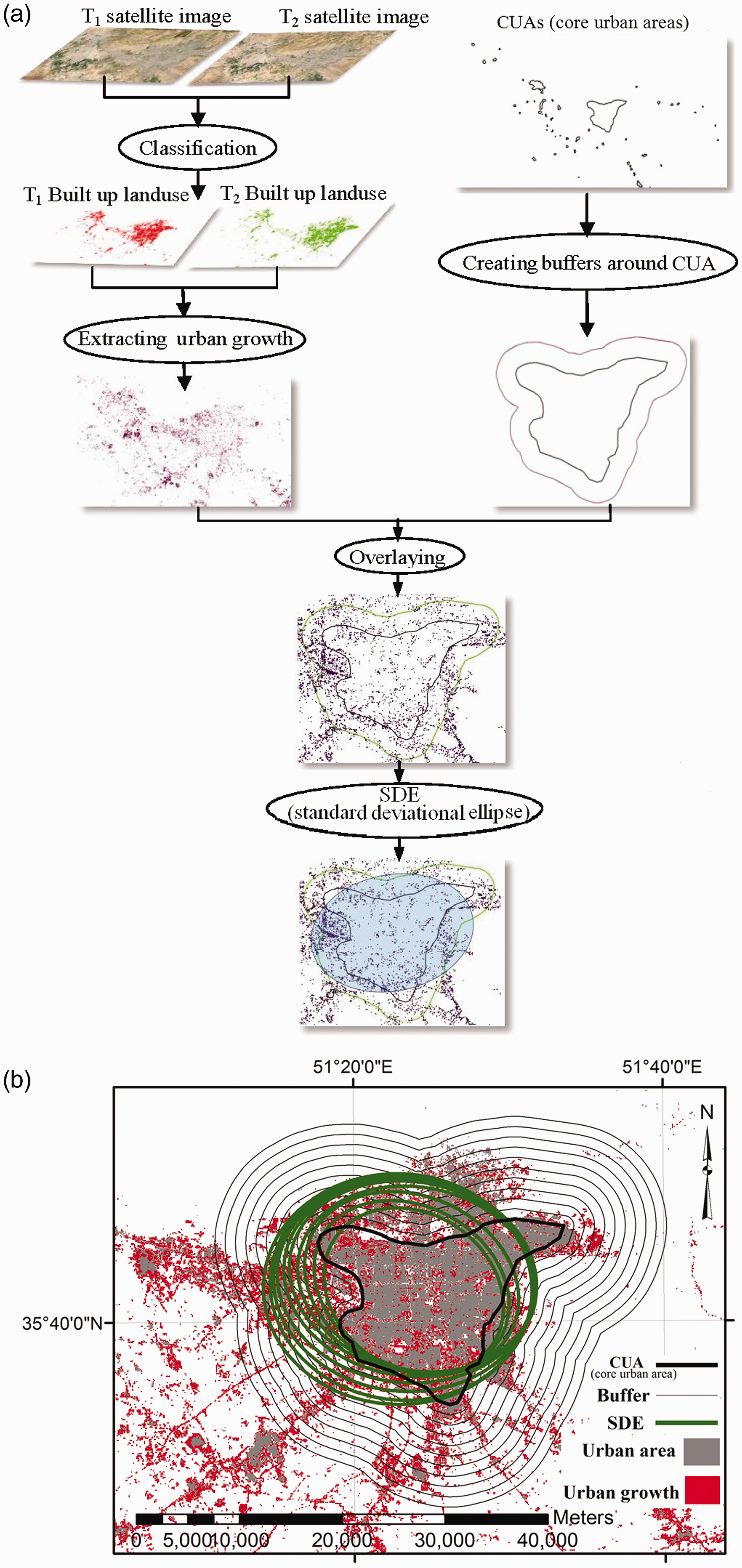
(a) Stages of fitting a standard deviational ellipse (SDE) on grown points around the core urban area (CUA) and (b) Fitting the SDEs on urban grown points in the interval buffers around the CUA of a city.

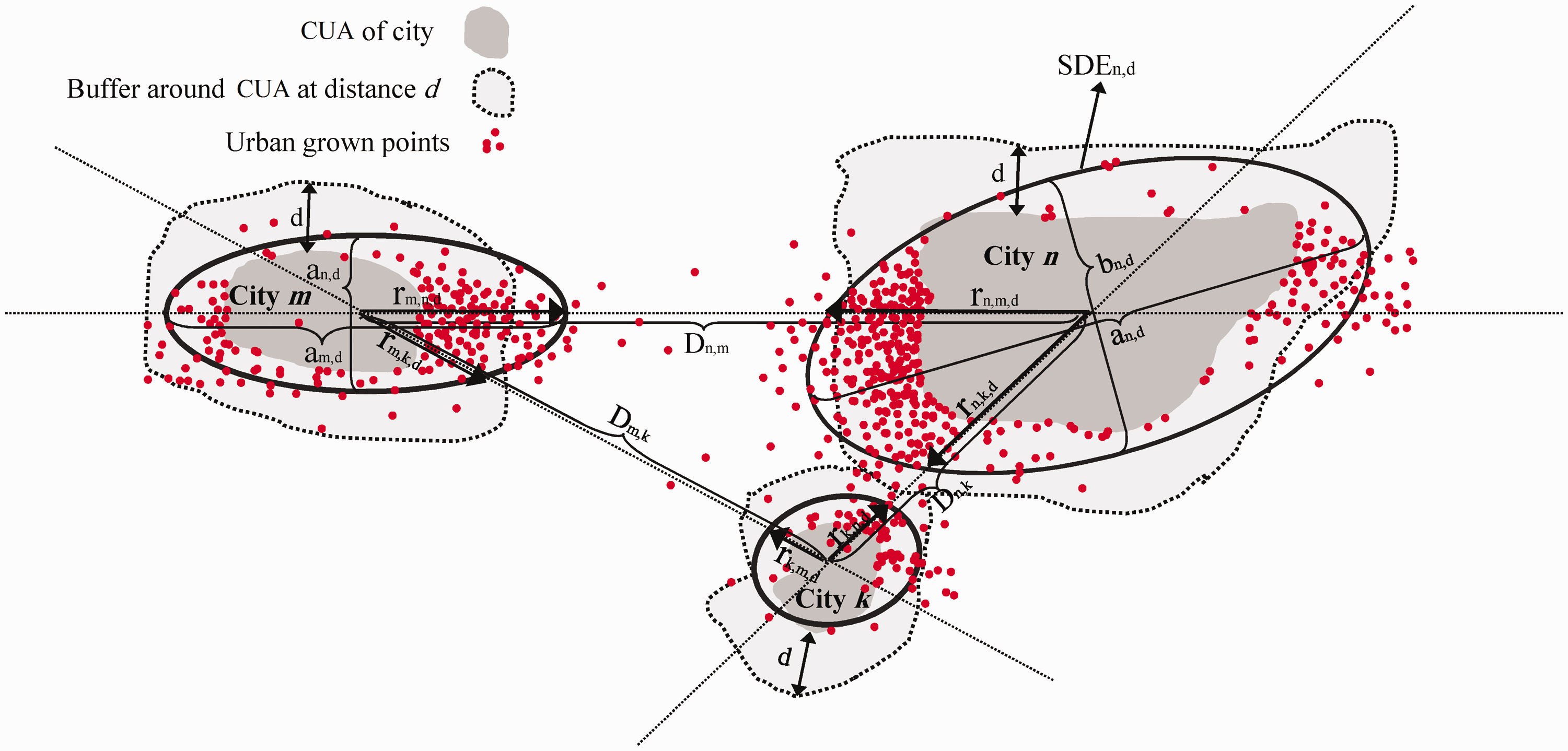
Based on the SDE parameters, the following equation is proposed to measure the DTUG that is due to the influence of city m on the urban growth of city n at a distance of d from city n

D T U G_{n, m, d} = \frac{r_{n, m, d} * G_{d}}{f_{n, d} * D_{n, m}}

(1)

f_{n, d} = b_{n, d} / a_{n, d}

(2)

Consider SDE_n,d as the SDE fitted on the urban points inside a buffer zone at distance d around the city n. Accordingly, $r_{n, m, d}$ is a diameter of SDE_n,d that is in the direction of city m, $f_{n, d}$ is the ratio of the length of the minor diameter of the SDE_n,d (b_n,d) to the length of the major diameter (a_n,d), $G_{d}$ is the urban growth rate at the buffer distance of d around the city n, where $G_{d}$ is measured based on the proportion of areas under urban growth and the area of buffer, excluding the CBD, and $D_{n, m}$ is the normalized distance between the centre of the SDE_n,d and the city m. The above parameters are shown schematically in Figure 2. Higher values of $D T U G_{n, m, d}$ represent a greater effect of the city m on the city n.

Figure 2.

The parameters of the DTUG indicator.

The four main parameters for measuring the $D T U G_{n, m, d}$ are $r_{n, m, d}$ , $G_{d}$ , $f_{n, d}$ and $D_{n, m}$ (r, G, f and D in the abstract). A conceptual model was provided to illustrate the role of each parameter of equation (1) in reflecting the directional trend of the urban growth of a city, as shown in Figure 3. Four scenarios were defined based on the four parameters. In each scenario, one parameter was changed and the other three were kept constant. In other words, this figure represents the way in which each parameter can reflect the influence of city m on city n. For instance, the first scenario (S1) supposes that there are three different states of distribution of the urban growth around city n and G, f and D are constant in the three times. In state one, the fitted SDE shows that the distribution of urban growth is almost horizontal (along the connection line between the two cities). However, in state three, the fitted SDE shows that the distribution of urban growth is almost vertical and in state two, the distribution of urban growth is diagonal. This reveals that the influence of city m on city n at time one (DTUG₁) is more than it is at time two and time three. Thus, it can be seen that the value of r in time one (r₁) is greater than in r₂ and r₃.

Figure 3.

The relative values of the DTUG in various scenarios.

The spatial interactions between the cities

In the study area, a location i is affected by the spatial interactions among the surrounding cities. The DTUG of different cities was integrated to measure the SIBC. It was supposed that i was at a distance of d from the city n. We then measured the total influence of other cities on the urban growth of city n at location i as follows

T D T U G_{n} (i) = \sum_{m = 1}^{k} \frac{D T U G_{n, m, d}}{(d i s t_{m, i} + d i s t_{n, i})}

(3)

where

d i s t_{m, i}

is the distance of i from the mth city. Now consider that the location i is at a distance of d₁, d₂, … d_n from city 1, city 2, … city n. First, we measured the related T

D T U G

₁(i), T

D T U G

₂(i), … and T

D T U G

_n(i). Second, the SIBC factor in the location i was defined as the maximum influence that cities exert on each other (Wang et al., 2011). For example, consider there are three cities in the study area. Thus, i is affected by the influence of each city on the other two to the extent of

T D T U G_{1} (i)

T D T U G_{2} (i)

and

T D T U G_{3} (i)

. Their maximum value will then be considered as IUF(i) (equation (4))

I U F (i) = max {T I_{1} (i), T I_{2} (i), \dots}

(4)

In addition, comparison of the results of the SIBC was calculated based on a GFM as follows (He et al., 2008, 2013)

t_{n, x, y} = \frac{F_{n}}{D_{(x, y, x_{n}, y_{n})}}

(5)

where

t_{i, x, y}

is the intensity of the influence of city n at cell (x,y);

D_{(x, y, x_{n}, y_{n})}

is the Euclidean distance from the city centre (

x_{n}, y_{n}

) to the cell (x, y); and

F_{n}

is the urban outflow from city n. In this study,

F_{n}

is the population of city n as a socio-economic factor.

Modelling the urban growth

Logistic-CA is one of the popular CA models for simulating urban land-use dynamics (Van Dessel et al., 2011) that was employed to simulate the urban growth in this study using the following equation

p_{i}^{0} = \frac{e^{z}}{1 + e^{z}} z_{i} = b_{0} + b_{1} x_{i}^{1} + b_{2} x_{i}^{2} + \dots . b_{n} x_{i}^{n}

(6)

$p_{i}^{0}$ is the potential for transforming a non-urban cell into an urban cell, ranging from 0 to 1. The factors ( $x_{i}^{n}$ ) include the SIBC, access to CUAs, highways, streets and major industrial zones, slope, height and the land-uses of neighbouring cells. These are normalized between 0 and 1. $b_{i}$ represents the coefficients of these factors. Taking into account the restriction on growth and the random variable, the above equation is amended as follows

P_{i} = p_{i}^{0} \times (1 + {(- l n γ)}^{α}) \times Ω_{i}

(6)

$Ω_{i}$ may assume 0 or 1, where 0 reflects the growth restrictions in cell i, $γ$ is a uniform random variable within the range of 0 – 1 and α is a parameter to control the size of the stochastic perturbation and its value is considered to be 0.3 on the basis of the radial dimension (Barredo et al., 2003).

The demand for urban land was estimated based on a linear regression of the historical data of the urban growth areas and the population. The urban growth map was then obtained according to the following equation (Lin and Li, 2015)

S_{i}^{t} = {\begin{array}{l} 1 & p_{i} \geq Threshold \\ 0 & p_{i} \leq Threshold \end{array}

(8)

If $S_{i}^{t}$ is equal to 1, the cell status will be converted into urban; otherwise, it will retain its previous land-use. The threshold of each step is specified according to the demand area. The figure of merit (FOM) was used to validate the modelling results (Pontius et al., 2008). In addition, we compared the results of the model that included the SIBC factor based on the proposed method (Logistic_CA_ SIBC), the GFM (Logistic_CA_GFM) and a similar model that did not consider this factor (Logistic_CA).

The study area and materials

The study area

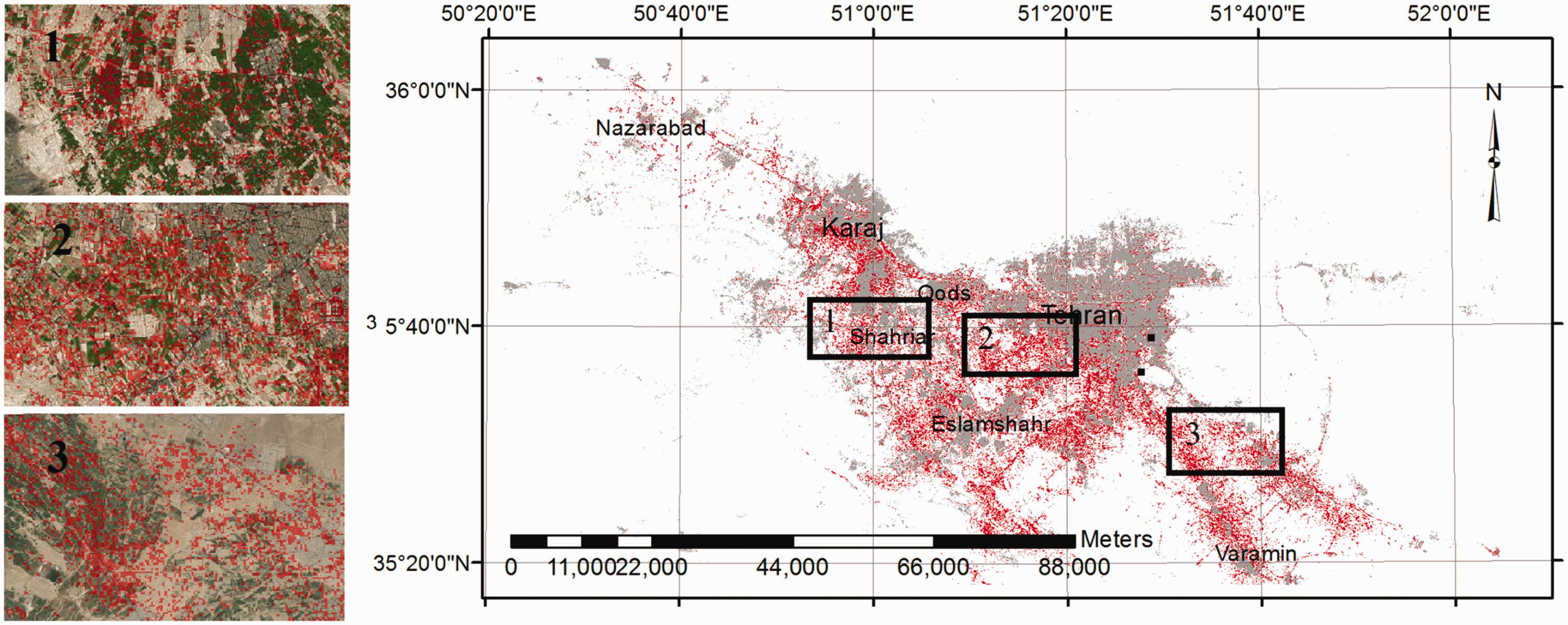
The TMR is located in the north of the central plateau of Iran, and it includes Tehran as the capital of Iran and one of the cities with the largest annual growth in Asia (World Gazetteer, 2012; Figure 4). The study area consists of Tehran and Alborz provinces, and covers a total area of 18,102 km², and the population reached 14.5 million in 2013. This region houses approximately 20% of Iran’s population and is the most industrialized region in Iran. Job opportunities, health and education services, and social welfare have led to widespread migration from all over the country to Tehran and the other cities in the study region (Sintusingha and Mirgholami, 2013; Tayyebi et al., 2011). Tehran’s population has overflowed in the last few decades into the surrounding cities due to high costs of living, severe traffic jams and air pollution in Tehran (Lalehpour, 2016).

Figure 4.

The limit of the TMR and counties.

Data collection

Land-use/cover maps for 1991, 2000, 2007 and 2014 were produced from the classification of Landsat 4, 5, 7 and 8 satellite images. The images were classified into six land-use/cover classes (built up, forest, water, arid, farmland, and mountain) using ENVI. To classify the images we selected 300 training samples and 300 test samples from the study area. Each sample formed a polygon around an area with a specific land-use. Therefore, each sample contained many cells. Classification was used for the training samples. We then reclassified the classes into two categories: urban and non-urban. Test samples were used to test the accuracy of the classification. The Kappa coefficient was calculated by comparing the land-use of the test samples with the land-use in the reclassified image. The Kappa coefficients were 0.84, 0.86, 0.85 and 0.87 for the years 1991, 2000, 2007 and 2014, respectively.

The CUA of the cities were manually plotted on the map with the help of expert knowledge. The neighbourhood effect map was obtained based on the number of urban land-uses in a window around the cells. Three-by-three, five-by-five and seven-by-seven window sizes were applied to examine the robustness of the logistic regression coefficients to window sizes. Moreover, the vector map of the transportation network and the parcel land-use map of the TMR were used to produce a highway, streets, major industrial and growth restrictions map. The rasterized digital terrain map (prepared by the National Cartographic Center of Iran) was used to prepare the slope and height maps. Figure 5 displays the factor maps. Based on previous studies and on the testing of different pixel sizes, a cell size of 100 m was considered to be best.

Figure 5.

The factor maps of urban growth, (a) proximity to CUAs, (b) proximity to highways, (c) proximity to streets, (d) proximity to major industries, (e) height, (f) slope and (g) local neighbourhood effect.

Implementation

Measuring and analysing the DTUG

The cities in the TMR were divided depending on their populations into four categories. (1) Tehran, (2) Karaj, (3) major cities (with a population more than 200,000 people) and (4) small cities (with a population less than 200,000 people). The DTUG values were obtained at various distances for each category using equation (1). Results have been displayed as graphs in Figure 6. In these graphs, the DTUG values at various distances from cities of each category are presented comparatively. For instance, a, b and c graphs illustrate the DTUG due to the effect of different cities on Tehran. Moreover, d, g and k graphs cover the influence of Tehran on the growth of other cities. In the calculation of DTUG of Tehran due to the major cities, the mean value of the DTUGs of four nearest major cities was considered. Similarly, the mean value was applied to other categories that have more than one city.

Figure 6.

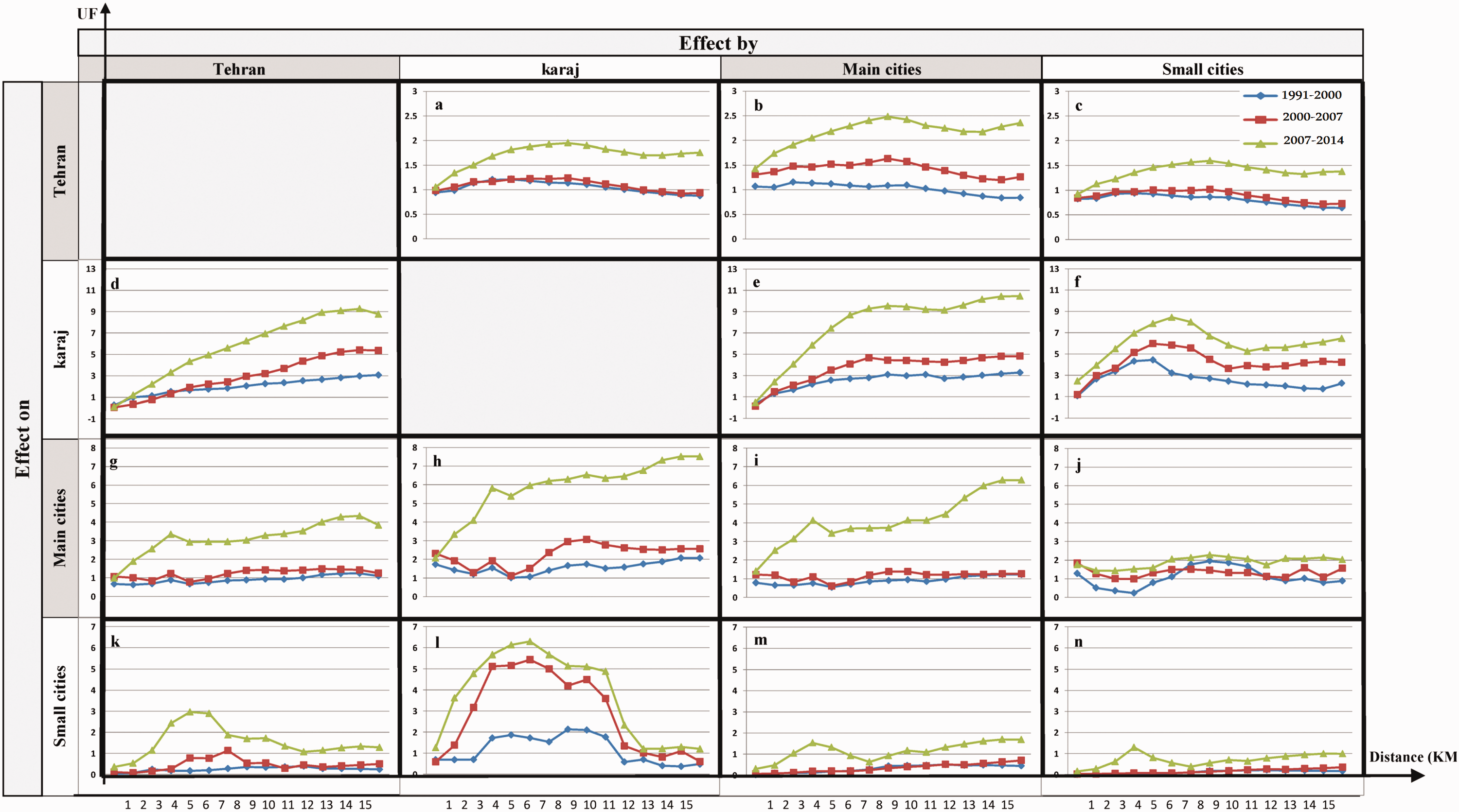
Spatio-temporal variations of the DTUG of four categories of the cities in the TMR.

In accordance with the graphs a, b and c, the expansion of Tehran tended toward the major cities. Such influence initially intensified farther away from the core area of Tehran and then gradually diminished. According to graphs d, g and k, Tehran had the greatest impact on Karaj and other major cities. Urban growth in Karaj was heavily influenced by Tehran and the neighbouring major cities. Karaj greatly affected the growth of major and small cities, where the most intense interactions in the region can be found. The major cities grew quite independently during 1991–2000 and 2000–2007 but, over time, they were influenced by their neighbouring cities. The periphery areas of small cities grew rather intensely toward Tehran, and Karaj, which was approximately independent of the surrounding major and small cities.

The graphs indicate that the interactions between the cities are asymmetric. However, a common feature shown in the graphs is that the DTUG increases over time. Moreover, the DTUG often intensifies on the periphery of the CUAs and overall growth has taken a southeast-northwest trend, and urban growth has further intensified toward the southern part of the region.

Calculating the SIBC

Using equations (3) and (4), the SIBC was calculated. First, to calculate the TDTUG, the DTGU values were extracted from the graphs that were based on the distance of a location from the cities. The TDTUG map derived for each category of cities is illustrated in Figure 7(a) and (b). Second, the maps of the SIBCs were derived using equation (4) (Figure 7(c)).

Figure 7.

The TDTUG map of each category of cities in (a) 2000–2007, (b) 2007–2014 and (c) the factor map of the SIBC.

These maps are more realistic than those derived from previous studies (He et al., 2013; Liang, 2009). As shown in Figure 7, in contrast to the results of previous methods, the influence of a city may not be identical in various directions around it or may not follow the distance decay relationship. In addition, the intensity of the SIBC generally increased between 2007 and 2014 compared to 2000 and 2007. During 2000–2007, the most intense SIBCs were found on the southern edge of Tehran and the central area of Karaj, whereas there were no significant interactions in other regions. However, during 2007–2014, the SIBC covered a wider area. Over the same period, the SIBC tended to be more intense in the southern half of Karaj and the west and southwest of Tehran, as well as the periphery of major and smaller cities. There were intense interactions between Karaj and its surrounding cities, as well as those that surround Tehran.

Model calibration and urban growth simulation

The coefficients of the models were calibrated using training samples for the two periods of 2000–2007 and 2007–2014. The coefficients were calibrated based on 5000 urban points and 5000 non-urban points as training data developed in each period. A training sample includes the value of the dependent variable (in this study it is 0 or 1 for urban or non-urban, respectively) and the values of the independent variables (in this study, distance to CBD, highways, slope, etc. in the location of the sample point). A 100 × 50 grid was fitted to the study area and for each cell of the grid one random urban growth point and one random non-urban point were selected. We used Pearson correlation coefficients to test the correlation between the factors (Table 1). The coefficients show that there were no significant correlations between the factors. Therefore, we were able to use all the factors in the modelling. The coefficients are presented in Table 2.

Table 1.

The Pearson correlation coefficients for the urban growth factors.

Factors	Proximity to CUAs	Proximity to highways	Proximity to main streets	Proximity to industrial regions	Slope	Height	Neighbour effect	SIBC
Proximity to CUAs	1.000	0.076	0.084	0.009*	0.053	−0.016*	−0.012*	−0.092
Proximity to highways	0.076	1.000	0.184	0.082	0.076	0.033*	0.006*	−0.092
Proximity to main streets	0.084	0.184	1.000	−0.042	0.155	−0.026*	−0.026*	−0.095
Proximity to industrial regions	0.009*	0.082	−0.042	1.000	−0.050	0.050	−0.069	0.006*
Slope	0.053	0.076	0.155	−0.050	1.000	0.051	0.209	−0.017*
Height	−0.016*	0.033*	−0.026*	0.050	0.051	1.000	0.102	0.016
Neighbourhood effect	−0.012*	0.006*	−0.026*	−0.069	0.209	0.102	1.000	0.058
SIBC	−0.092	−0.092	−0.095	0.006*	−0.017*	0.016*	0.058	1.000

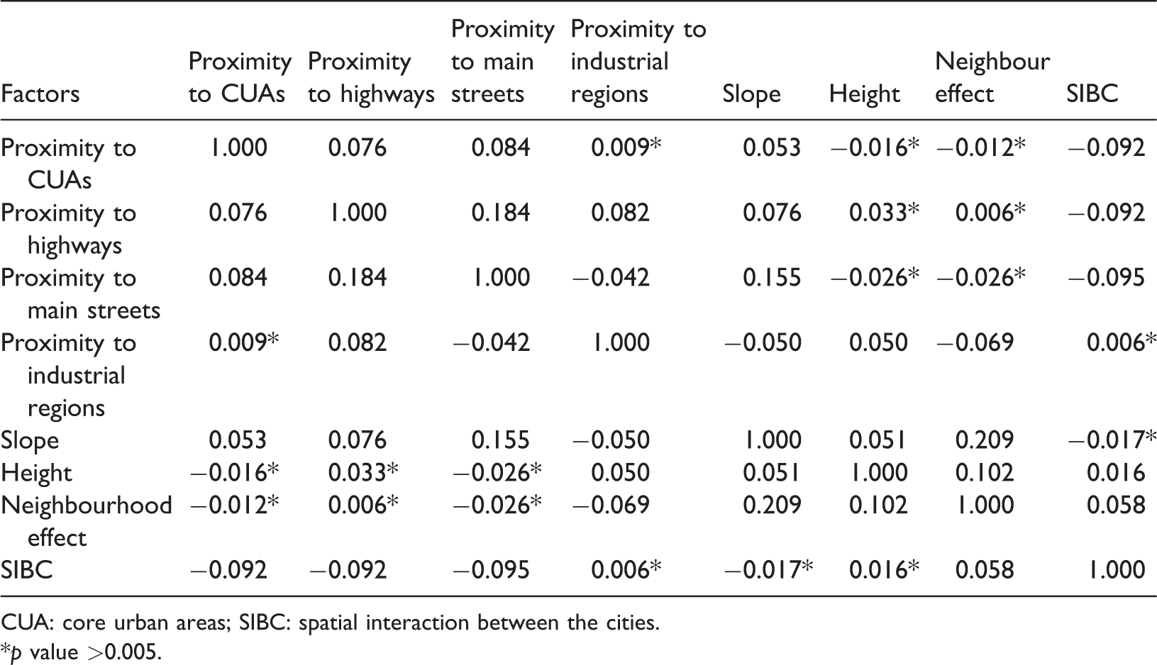
CUA: core urban areas; SIBC: spatial interaction between the cities.

*p value >0.005.

Table 2.

The coefficients of Logistic_CA_SIBC, Logistic_CA and Logistic_CA_GFM models.

	Logistic_CA_SIBC						Logistic_CA						Logistic_CA_GFM
	Neighbourhood effect windows size						Neighbourhood effect windows size						Neighbourhood effect windows size
	2000–2007			2007–2014			2000–2007			2007–2014			2000–2007			2007–2014
Factors	3 × 3	5 × 5	7 × 7	3 × 3	5 × 5	7 × 7	3 × 3	5 × 5	7 × 7	3 × 3	5 × 5	7 × 7	3 × 3	5 × 6	7 × 7	3 × 3	5 × 5	7 × 7
Intercept	1.161	1.172	1.173	1.189	1.200	1.204	1.297	1.362	1.296	1.344	1.348	1.319	1.202	1.180	1.181	1.172	1.210	1.165
Proximity to CUAs	−0.931	−0.946	−0.946	−0.280	−0.283	−0.279	−1.363	−1.364	−1.357	−0.576	−0.581	−0.564	−1.042	−1.038	−1.035	−0.461	−0.466	−0.468
Proximity to highways	−3.876	−3.887	−3.886	−1.901	−1.923	−1.924	−3.834	−3.841	−3.853	−1.777	−1.794	−1.794	−3.772	−3.760	−3.755	−1.885	−1.893	−1.904
Proximity to main streets	−1.078	−1.099	−1.094	−1.032	−1.046	−1.047	−1.236	−1.223	−1.216	−1.158	−1.149	−1.148	−1.102	−1.111	−1.108	−1.092	−1.054	−1.054
Proximity to industrial regions	−0.824	−0.828	−0.829	−0.936	−0.956	−0.956	−1.048	−1.065	−1.069	1.717	1.707	1.707	−1.046	−1.054	−1.058	−1.110	−1.117	−1.119
Slope	−10.183	−10.118	−10.067	−16.706	−16.720	−16.713	−10.200	−10.211	−10.191	−17.031	−17.042	−17.010	−9.873	−9.875	−9.789	−14.981	−14.975	−14.891
Height	−0.431	−0.425	−0.427	−0.529	−0.541	−0.543	0.0537	0.0539	0.0533	−0.168	−0.170	−0.170	−0.513	−0.509	−0.507	−0.524	−0.532	−0.528
Neighbourhood effect	2.920	2.910	2.909	1.865	1.863	1.863	2.843	2.841	2.846	1.913	1.910	1.900	2.892	2.889	2.873	2.125	2.129	2.120
SIBC	1.127	1.122	1.123	1.387	1.388	1.379	–	–	–	–	–	–	0.811	0.795	0.795	0.954	0.913	0.966

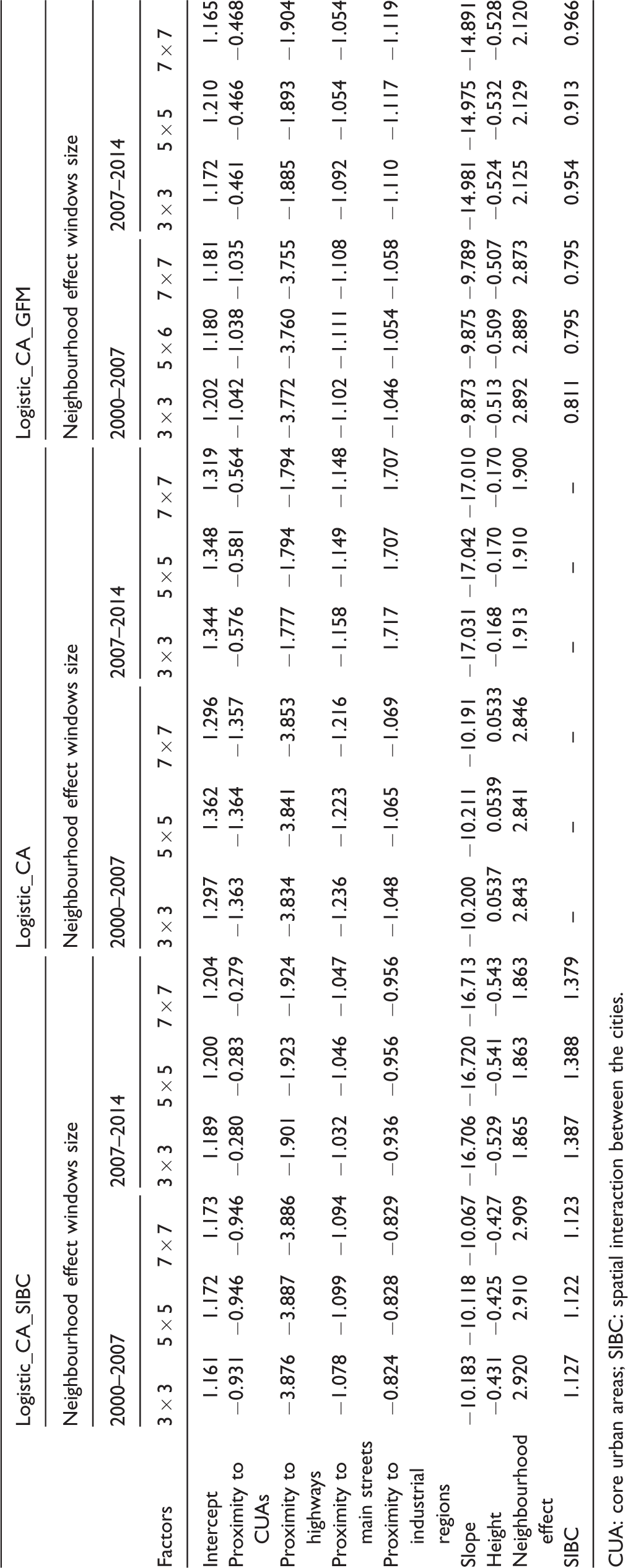
CUA: core urban areas; SIBC: spatial interaction between the cities.

As shown in Table 2, the SIBC is one of the important driving forces. This factor significantly increased during 2007–2014 compared to 2000–2007. We used the calibrated coefficients of the models in the 2000–2007 period to simulate urban growth in 2014. The potential for urban growth was calculated using equations (6) and (7). On the other hand, the urban demand area in 2014 was extracted from the classified images of 2014. The demand area is 353.75 km². We then selected a threshold for classifying the urban growth potential map into two, urban and non-urban classes using equation (8). The potential threshold was adjusted based on a trial/error method by considering the demand area. The simulated urban growth maps were produced using Logistic_CA, Logistic_CA_SIBC and Logistic_CA_GFM models and all three different window sizes for the neighbourhood effect were taken into account. Figure 8 shows the simulated urban growth maps in 2014 using the window size of 5 × 5 for the neighbourhood effect.

Figure 8.

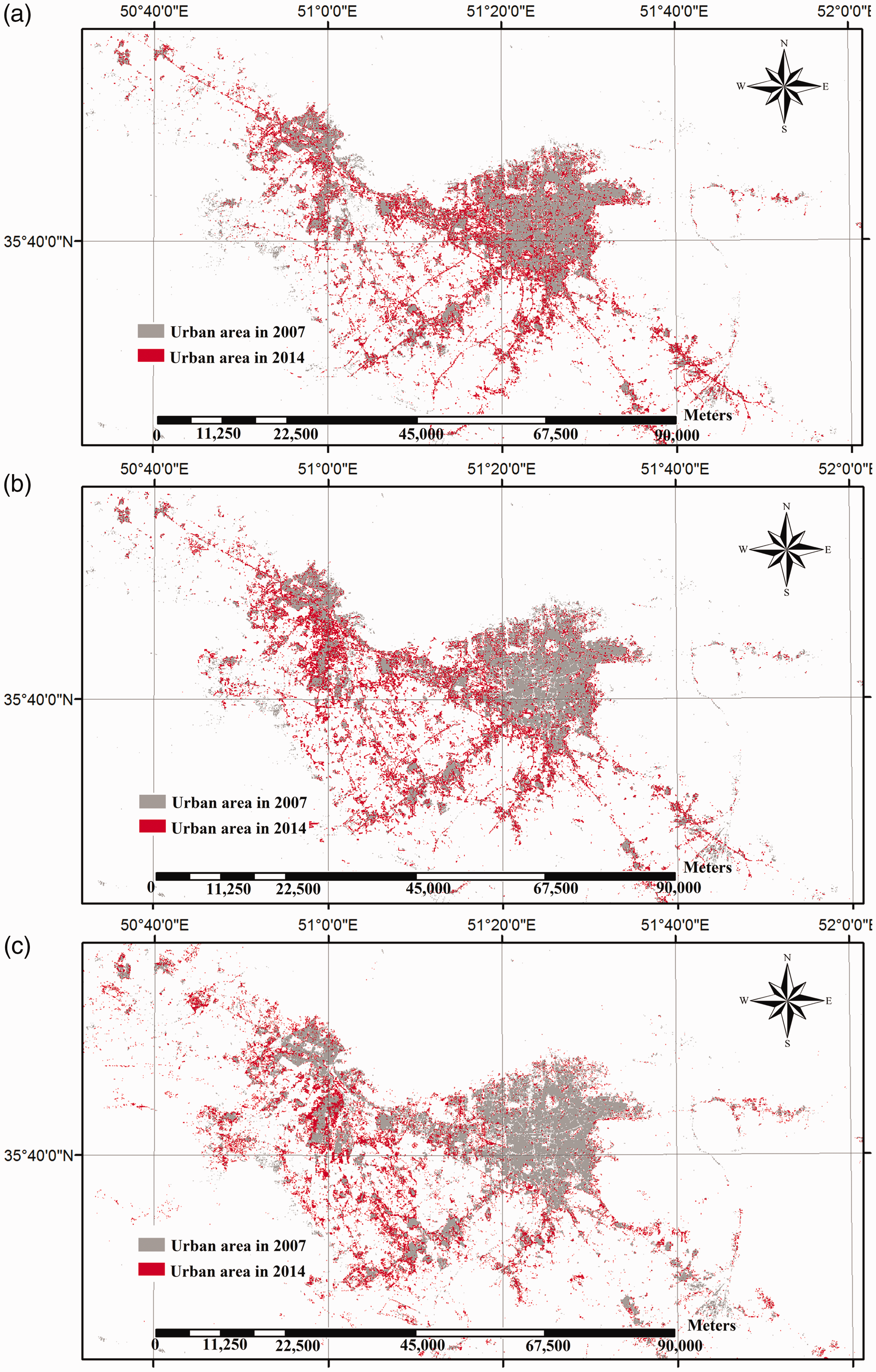
The simulated urban growth map (a) using the Logistic_CA, (b) using the Logistic_CA_SIBC and (c) the actual urban growth in 2014.

The validation results and prediction of urban growth

We compared the urban growth maps produced with the Logistic_CA, Logistic_CA_SIBC and Logistic_CA_GFM models with actual urban growth up to 2014. The FOM values were then calculated. The FOM values for the models at three different window sizes are presented in Table 3. The window size of 5 × 5 results was best for the FOMs. The FOM values for the Logistic_CA, Logistic_CA_SIBC and Logsitic_CA_GFM models were 18.55%, 24.99% and 20.70%, respectively. The above values represent more accurate results of the urban growth modelling (6.44%) by including the SIBC factor developed in this study and 2.15% better results by including the SIBC calculated on the basis of GFM.

Table 3.

The FOM values for results of Logistic_CA_SIBC, Logistic_CA and Logistic_CA_GFM models.

	Logistic_CA_SIBC			Logistic_CA			Logistic_CA_GFM
	3 × 3	5 × 5	7 × 7	3 × 3	5 × 5	7 × 7	3 × 3	5 × 5	7 × 7
FOM (%)	24.67	24.99	24.56	18.58	18.55	18.47	20.59	20.70	20.71
Average (%)		24.74			18.53			20.66

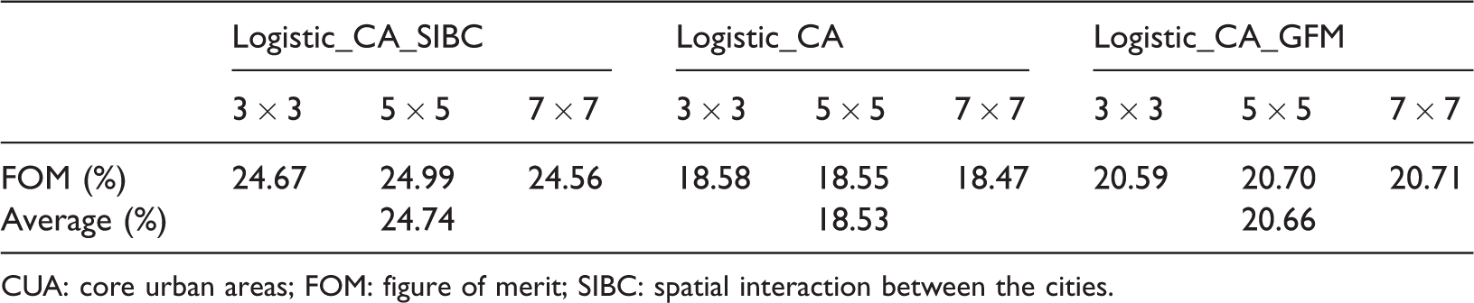
CUA: core urban areas; FOM: figure of merit; SIBC: spatial interaction between the cities.

For predicting urban growth in 2021, the urban demand area was estimated. Assuming the existing growth rate will continue, a linear regression was employed to calculate the total urban areas by 2021. The urban growth map for the TMR is simulated using the Logistic_CA_SIBC as shown in Figure 9. According to this map, the urban growth trend is to the south and southwest. There is a remarkable growth found in cities located in the southern and south-western areas of Tehran and southern and southeast of Karaj. It is seen that the process of urban development in this region is in the diffusion phase. If the current trend persists, the farmlands and green spaces across the southern areas of Karaj will vanish one after another. Another urban growth wave will be initiated in south-eastern Tehran forming a corridor trend near the main road. Moreover, the growth rate of Tehran will be greater in suburban areas.

Figure 9.

Urban growth prediction of the TMR in 2021.

Conclusion and discussion

In this study, we try to measure the SIBC based on measuring the DTUG using spatial statistics and the history of urban land change extracted from satellite images. Then, we consider it in the urban growth modelling.

The spatiotemporal analysis of the DTUGs characteristics in the TMR during the periods 1991–2000, 2000–2007 and 2007–2014 provided the potential to explore the urban growth pattern and processes. The overall growth trend of the study area covers the southeast-northwest alignment of the Tehran–Karaj–Qazvin axis. The results indicate that DTUG mostly peaked on the periphery of the CUAs. The expansion of Tehran tended toward the surrounding major cities. Moreover, due to the influence of Tehran on major cities, the DTUG peaked in its suburbs. Tehran had the greatest effect on the expansion of Karaj and major cities. Karaj largely led the growth of its surrounding small and large cities and the most intense SIBC can be found in this area. The expansion of the major cities was quite independent during 1991–2000 and 2000–2007. However, they were affected by their surrounding cities over time. The small cities expanded rather intensely toward Tehran, and particularly Karaj, and were almost independent of the surrounding major and small cities.

Unlike previous studies (He et al., 2013; Lin and Li, 2015), the results indicate that the SIBC varies in terms of direction and distance around the cities. This is because the influence of a city on the urban growth of its surrounding cities does not necessarily follow the distance decay effect (Tiefelsdorf, 2003), and may not necessarily be the same in the different directions of a city (radial effect; Lin and Li, 2015). Figure 8 demonstrates there are intense spatial interactions across the middle and southern parts of Karaj. Over time, the SIBC accelerated and expanded over the region.

A CA-based logistic regression model was used to evaluate the role of the SIBC in urban growth modelling. By considering the SIBC factor, the FOM of the results increased by 6.44%. The results show the SIBC increase the urban growth potential and its role in modelling becomes more important over time. In addition, we used the GFM to model interactions between the cities based on the population data of cities, which was incorporated into the Logsistic_CA model. The results show that the accuracy of this model increased by 2.15%. The difference between the two values of improved accuracy (6.5% and 2.15%) confirmed that the SIBC reflects the influence of some socio-economic factors, such as population, growth domestic product (GDP) and the level of service, which considering just one of them in the modelling slightly increased the accuracy. Instead, the directional trends of urban growth are considered as the consequence of these interactions between the cities for reflecting its influence of it.

The results indicate that the proposed methodology can provide a tool for planning the development of metropolitan regions. Moreover, analysing the spatiotemporal characteristics of the DTUG will reveal the results of development policies and help urban managers to make better decisions for the future of the metropolitan regions. For example, this may be useful when developing policies that determine land-use, such as facilities with a regional function that serve more than one city, making decisions about issues related to the urban flows or determining the cities’ sphere of influence.

It is recommended that future research implements the proposed model in other metropolitan regions and simulates urban growth in different scenarios. In addition, because of the experimental nature of the proposed indicator for the quantification of the SIBC, it is suggested that future research should involve a sensitivity analysis by changing its parameters. Finally, the size and shape of the CUA may impact on the ellipse parameters. So, we propose to investigate the relation between them in future research.

Footnotes

Declaration of conflicting interests

The author(s) declared no potential conflicts of interest with respect to the research, authorship, and/or publication of this article.

Funding

The author(s) received no financial support for the research, authorship, and/or publication of this article.

Sanaz Alaei Moghadam graduated from Khaje Nasire Din Toosy University in GIS field and she is working in a municipality as an urban administrator.

Mohammad Karimi graduated from the Khaje Nasire Din Toosy University in GIS field and he is an assistant professor in this university.

Kyoumars Habibi graduated from Iran University of Science & Technology in the urban planning field and he is an assistant professor in the Kurdistan University.

References

Al-Shalabi

Billa

Pradhan

, et al. (2013) Modelling urban growth evolution and land-use changes using GIS based cellular automata and SLEUTH models: The case of Sana’a metropolitan city, Yemen. Environmental and Earth Science 70(1): 425–437.

Barredo

Kasanko

McCormick

, et al. (2003) Modelling dynamic spatial processes: Simulation of urban future scenarios through cellular automata. Landscape and Urban Planning 64(3): 145–260.

Chen

Liu

, et al. (2013) Modeling urban land-use dynamics in a fast developing city using the modified logistic cellular automaton with a patch-based simulation strategy. International Journal of Geographical Information Science 28(2): 234–255.

Dietzel

Oguz

Hemphill

, et al. (2005) Diffusion and coalescence of the Houston Metropolitan Area: Evidence supporting a new urban theory. Environment and Planning B 32(2): 231–246.

Favaro

Pumain

(2011) Gibrat revisited: An urban growth model incorporating spatial interaction and innovation cycles. Geographical Analysis 43(3): 261–286.

Fragkias

Seto

(2009) Evolving rank-size distributions of intra-metropolitan urban clusters in South China. Computers, Environment and Urban Systems 33(3): 189–199.

Gonzalez

Aguilera-Benavente

Gomez-Delgado

(2015) Partial validation of cellular automata based model simulations of urban growth: An approach to assessing factor influence using spatial methods. Environmental Modelling & Software 69: 77–89.

He Ch, Okada N, Zhang Q, et al. (2008) Modelling dynamic urban expansion processes incorporating a potential model with cellular automata. Landscape and Urban Planning 86(1): 79–91.

He Ch Zhao

Tian

, et al. (2013) Modelling the urban landscape dynamics in a megalopolitan cluster area by incorporating a gravitational field model with cellular automata. Landscape and Urban Planning 113: 78–89.

10.

Karimi

Mesgari

Sharifi

, et al. (2017) Developing a methodology for modelling land-use change in space and time. Journal of Spatial Science 62(2): 1–20.

11.

Lalehpour

(2016) Recognition of management structure and spatial planning in Tehran metropolitan area. Journal of Urban Management 5(1): 3–15.

12.

Lefever

(1926) Measuring geographic concentration by means of the standard deviational ellipse. American Journal of Sociology 32(1): 88–94.

13.

(2013) Quantifying the speed, growth modes, and landscape pattern changes of urbanization: A hierarchical patch dynamics approach. Landscape Ecology 28: 1875–1888.

14.

Liang

(2009) Research on the urban influence domains in China. International Journal of Geographical Information Science 23(12): 1527–1539.

15.

Lin

(2015) Simulating urban growth in a metropolitan area based on weighted urban flows by using web search engine. International Journal of Geographical Information Science 29(10): 1721–1736.

16.

Liu

, et al. (2014) Simulating urban growth by integrating landscape expansion index (LEI) and cellular automata. International Journal of Geographical Information Science 28(1): 148–163.

17.

Myint

(2008) An exploration of spatial dispersion, pattern, and association of socio-economic functional units in an urban system. Applied Geography 28: 168–188.

18.

Pontius

Boersma

Castella

, et al. (2008) Comparing the input, output, and validation maps for several models of land change. The Annals of Regional Science 42(1): 11–37.

19.

Sarvestani

Latif Ibrahim

Kanaroglou

(2011) Three decades of urban growth in the city of Shiraz, Iran: A remote sensing and geographic information systems application. Cities 28: 320–329.

20.

Seto

Reenberg

Boone

, et al. (2012) Urban land teleconnections and sustainability. Proceedings of the National Academy of Sciences 109(20): 7687–7692.

21.

Sintusingha

Mirgholami

(2013) Parallel modernization and self-colonization: Urban evolution and practices in Bangkok and Tehran. Cities 30: 122–132.

22.

Taubenböck

Wienser

Felbier

, et al. (2014) New dimensions of urban landscapes: The spatio-temporal evolution from a polynuclei area to a mega-region based on remote sensing data. Applied Geography 47: 137–153.

23.

Tayyebi

Pijanowski

B Ch

Pekin

(2011) Two rule-based urban growth boundary models applied to the Tehran. Applied Geography 31: 908–918.

24.

Tiefelsdorf

(2003) Misspecifications in interaction model distance decay relations: A spatial structure effect. Journal of Geographical Systems 5(1): 25–50.

25.

Van Dessel

Van Rompaey

Szilassi

(2011) Sensitivity analysis of logistic regression parameterization for land-use and land cover probability estimation. International Journal of Geographical Information Science 25(3): 489–508.

26.

Wang

Deng

Liu

, et al. (2011) Research on urban spheres of influence based on improved field model in central China. Journal of Geographical Sciences 21(3): 489–502.

27.

Wang

Shi

Miao

(2015) Confidence analysis of standard deviational ellipse and its extension into higher dimensional Euclidean space. PloS One 10(3): e0118537.

28.

Weber

Puissant

(2003) Urbanization pressure and modelling of urban growth: example of the Tunis Metropolitan Area. Remote Sensing of Environment 86(3): 341–352.

29.

White

Uljee

Engelen

(2012) Integrated modelling of population, employment and land-use change with a multiple activity-based variable grid cellular automaton. International Journal of Geographical Information Science 26(7): 1251–1280.

30.

World Gazetteer (2012) Available at: http://www.world-gazetteer.com/ (accessed 2012).

31.

Xiao

Wang

Liu

, et al. (2013) Reconstructing gravitational attractions of major cities in China from air passenger flow data, 2001–2008: A particle swarm optimization approach. The Professional Geoghrapher 65(2): 265–282.

32.

Zhu Y and Yu N (2002) Urban flows in the Hu Ning Hang urban compact district. Urban Planning Forum 1: 31–33.