Measuring McCities: Landscapes of chain and independent restaurants in the United States

Abstract

Urban planners have a stake in preserving restaurants that are unique to local areas in order to cultivate a distinctive, authentic landscape. Yet, over time, chain restaurants (i.e. franchises) have largely replaced independently owned restaurants, creating a landscape of placelessness. In this research, we explored which (types of) locales have an independent food culture and which resemble McCities: foodscapes where the food offerings can be found just as easily in one place as in many other (often distant) places. We used a dataset of nearly 800,000 independent and chain restaurants for the Continental United States and defined a chain restaurant using multiple methods. We performed a descriptive analysis of chainness (a value indicating the likelihood of finding the same venue elsewhere) prevalence at the urban area and metropolitan area levels. We identified socioeconomic and infrastructural factors that correlate with high or low chainness using random forest and linear regression models. We found that car-dependency, low walkability, high percentage voters for Donald Trump (2016), concentrations of college-age students, and nearness to highways were associated with high rates of chainness. These high chainness McCities are prevalent in the Midwestern and the Southeastern United States. Independent restaurants were associated with dense pedestrian-friendly environments, highly educated populations, wealthy populations, racially diverse neighborhoods, and tourist areas. Low chainness was also associated with East and West Coast cities. These findings, paired with the contribution of methods that quantify chainness, open new pathways for measuring landscapes through the lens of unique services and retail offerings.

Keywords

Chain restaurants independent restaurants franchises local culture placelessness

Introduction

Restaurants are valuable parts of the city, perpetuating foot traffic and urban spending (Credit and Mack, 2017) and simultaneously expressing and preserving local culture (Onesti, 2017). They are a common outing destination and invitation to engage in public recreational life (Rosenbaum, 2006). Restaurants are also micro-sensors of urban neighborhoods, reflecting the underlying socioeconomic attributes of places (Dong et al., 2019), intensity of local economic activities, consumption segregation, and local economic inequality (Glaeser et al., 2017; Moro, 2019).

Much of the American food consumption landscape consists of “chain” (i.e. franchised, multi-outlet) restaurants, as a result of globalization and the mass manufacturing of food and dining experiences (Kunstler, 1994). Chain restaurants, ranging from fast food such as McDonalds to exclusive outlets such as Morton’s Steakhouse, can provide convenient, familiar dining options to patrons. These restaurants exhibit similar signage and offerings across locales and are often owned by distant corporations, many of which own multiple brands of restaurants. These restaurants are also gaining popularity. During 2017–2018, there was a 4% increase in fast-casual chain restaurants and a 3% decline in U.S. independently owned restaurants (about 10,952 closings) in the United States (The NPD Group, 2018).

Because of their ubiquity, chains, alongside big box stores and chain hotels, counter the uniqueness of a landscape, producing a conceptual McCity.¹ A lack of uniqueness in a landscape is associated with mourning, feelings of loss, a lack of meaning, and lack of attachment for those who experience the locale (Arefi, 1999). Such landscapes have been referred to as non-place realms (Webber, 1964), or embodying the characteristic of placelessness (Relph, 1976). Visitors find difficulty forming memories of and envisioning future interactions with placeless locales (Milligan, 1998), thus dulling their experience of place and preventing the occurrence of meaningful experiences in the built environment (Arefi, 1999).

We currently lack methods to measure and detect placelessness in the foodscape, despite ample data on restaurant type and location. In response, we defined the concept of “chainness” through four different metrics, to provide a measurable indicator of placelessness from a consumer’s perspective. These metrics have a clear numeric range, and are designed to be useful for researchers, practitioners and popular audiences (as in Lopez and Hynes, 2003).

We used these metrics to answer the following research questions: Which cities and regions tend to have the highest chainness? What kinds of place characteristics (walkability, political behavior, socioeconomic variables) correlate with high chainness? Do chain restaurants tend to locate disproportionately near certain geographic features (e.g., waterways and highways)?

We used a dataset of nearly 800,000 restaurants in the Continental United States, supplied by the Yellow Pages. We assigned each restaurant a chainness score, which represents the restaurant frequency and expanse, and analyzed average chainness at various spatial levels. We then tested whether chainness correlates with place characteristics and distance to geographic features.

The outcome is a better understanding of the characteristics of places that support independent, unique venues and those that tend to resemble McCities, whose foodscape is overseen by a set of distant corporations. This knowledge can be useful for understanding how to monitor or mitigate placelessness, guide inclusive growth, and answer philosophical inquiries into the future of placemaking.

In the following section, we briefly describe the history of U.S. restaurants, the theory of placelessness, and prior work on spatial and demographic factors in restaurant location analysis. We then describe the dataset and methods, and report on findings. We conclude with a discussion that contextualizes our findings within concerns about food offerings and initiatives to mitigate placelessness.

Background

History of U.S. restaurants and urban culture

In the United States, many restaurants emerged from the Post-Second World War economic boom, as the service industry responded to new demand for high-end amenities (Zukin, 1998). These “consumption spaces” gradually replaced production spaces (i.e. factories) after the Industrial Revolution (Harvey, 1993; Lash and Urry, 1993; Miller, 1995; Mullins et al., 1999; Zukin, 1998) and encouraged the extensive consumption of goods and services, including dining outside the home (Bocock, 2008; Featherstone, 2007; Miller, 1995). With the rise of restaurants also came fast food and restaurant franchises, such as the classic midcentury example of Howard Johnson’s. These options arose amid increased train passage and car culture, as well as the growth of highway driving (Belasco, 1979), wherein travelers enjoyed a trusted brand away from home. In the 1970s, chain restaurants were also proposed as “cheap and quick” solutions to revitalize decaying urban areas and were marketed as entrepreneurial opportunities to African Americans (Small, 2017).

Beginning in the 1980s and 1990s, restaurants and bars in downtown areas attracted young, educated individuals with disposable income (Lees et al., 2013). Dual-career families tended to spend less time on cooking at home (Karsten et al., 2015), a departure from the consumption patterns of traditional suburban families of the past (Mullins et al., 1999). These trends demanded new consumption infrastructure dedicated to food and drinking spaces (Bridge and Dowling, 2001; Zukin, 2009). Today, cities also continue to need high-end restaurants to host business transactions, special occasions, and tourists (Jones et al., 2004). Yet, some cities rely on independently spirited, local restaurants to serve these purposes and others on high-end chain restaurants.

Landscape authenticity vs. placelessness

As landscape features, restaurants simultaneously embody and contribute to larger theories of place authenticity vs. placelessness. Place authenticity that can be classified as a “transmitter of values and significance of cultural landscape” (Nezhad et al., 2015: p. 93), and authentic architecture, foodways, and shopping outlets support the local economy and help conserve the traditional landscape (Sims, 2009; Trubek, 2008; Zeng et al., 2014). Authenticity also contributes to place attachment, as the sense of association between an individual and place influences well-being and mental health (Rivlin, 1982; Scannell and Gifford, 2010; Shumaker and Taylor, 1983). When applied to foodscapes, authenticity can be codified as recipes, menu items, decor, and the use of local culture to convey an experience (Cohen, 1988).

Landscape authenticity can be found in urban contexts, specifically walkable downtown areas with public spaces and pedestrian activities (i.e. “Main Streets”). These streets are alive with sights, sounds, and smells that engage patrons (Jones et al., 2016; Mullins et al., 1999) and reflect the identity of the locale through historic buildings, and visitor centers. They offer unique activities and services that differ from the big box warehouse and car-oriented suburban areas (Talen and Jeong, 2019a, 2019b). They also serve as landing destinations for out-of-town visitors, and are often cultivated as the image that the city wants its visitors to see (Talen and Jeong, 2019b). Independently run businesses help perpetuate this image and branding. Accordingly, we posit that dense downtowns will have more independent restaurants, and lower “chainness” scores.

Placelessness is a condition where the diversity or significance of a place has deteriorated (Relph, 1976), often associated with loss of meaning (Buttimer, 1980). Placelessness arose from “mass culture” movements that purport that individuals have similar needs that can be satisfied uniformly and with a similar style (Kruft, 1994). Mass construction of goods and infrastructure, as well as a globalized consumer supply chain, has produced a dull and globalized environment, perpetuating placelessness (Harvey, 1993; Zukin, 2009).

Today, despite the shuttering of many brick-and-mortar institutions, restaurants remain a key part of the built environment, and thus, an appropriate point of interest (POI) for investigation of placelessness. As entertainment options have moved to the home, the service industry has emphasized activities and experiences (Pine and Gilmore, 1998), and dining out is no exception. Independent restaurants are well-suited to provide this coveted experience and enhance the story of dining (Mossberg and Eide, 2017; Pine and Gilmore, 1998). This is particularly true in a recreational leisure setting, as independent restaurants are used to enhance the uniqueness of the vacation experience (Piramanayagam et al., 2020; Sands et al., 2015). Because of the demand for a unique experience, and the use of landscape authenticity in drawing tourists (Sharpley, 1994), we hypothesize that vacation or tourist areas will have many independent restaurants.

Spatial and demographic factors of restaurant location

Several models have been developed to address restaurant location decisions. Commonly used theories include central place theory, spatial interaction theory, and linear city model. These models help explain economic motivations behind the high concentration of fast food chains in heavy (car or foot) traffic areas and the decentralization of independently owned restaurants (Brown, 1993; Melaniphy, 1992). Fast food restaurants tend to cluster (Leslie et al., 2012), and road density tends to predict their presence (Teixeira et al., 2004). Commercial land use areas (Kwate et al., 2009), interstate highways, and arterial roads also attract chain restaurants (Carroll and Torfason, 2011; Hurvitz et al., 2009). Planning regulations such as zoning and parking requirements also privilege chains that tend to cluster and serve customers traveling by car (Shoup, 2005).

Prior studies on restaurants and sociodemographic groups have largely focused on the connection between restaurant placement, food offerings, and health (e.g., Morland et al., 2002). These studies have illustrated that lower income populations are susceptible to unhealthy fast food (Austin et al., 2005) or likely to live in food deserts (Beaulac et al., 2009). High-income communities have a high percentage of independent restaurants (Carroll and Torfason, 2011), and chain restaurants are said to appear more frequently in African American and low-income neighborhoods (Block et al., 2004). In the United States, increased fast food consumption is associated with factors such as male gender, older age, non-Hispanic black race/ethnicity, and residing in the South (Bowman et al., 2004).

Politics can also affect the local chainness. Negative consequences of poor food choice include poor nutrition and diabetes, but it is interpreted differently as to whether food choice is a personal responsibility or a public health concern that can be mitigated with better options and messaging (Frederick et al., 2016; Kersh, 2009). In the case of the latter, planning regulations can be enforced by promoting or combating zoning policies that regulate fast food industries. Bobrowski (2012) identified 28 cities, including Left-leaning areas in California and Massachusetts, with local zoning power to restrict “formula businesses.” These factors call for investigation into the correlation between residents’ political orientation and the chain foodscape more broadly. We expect the results of our socio-economic analysis to reflect the findings in this collective body of research.

Data and methods

Restaurants dataset

We gathered data on restaurant locations from the Yellow Pages (www.yellowpages.com) in 2016–2017 for the Continental United States by retrieving records from the pre-coded “Restaurant” search button/icon for each zip code. The Yellow Pages is a reliable source of restaurant data that has similar accuracy as Google Maps (Deng and Newsam, 2017). Our dataset includes restaurant names and street address. Restaurants are geolocated to the coordinate level using the Google Geocoding API. Restaurants with no address, no resultant geocoding coordinates, or duplicate listings (instances with the same restaurant name and address) were removed, reducing the dataset from over one million records to 793,322 records. The final dataset contained 437,073 unique restaurant names. We validated samples of our data manually (80% were found to exist on Google Maps in early 2021) and cross-checked the total numbers with other sources (82-92% maximum overlap) (see S.I. Section I).

Chainness definitions

We found no prior numerical definition of a chain restaurant with which to classify each restaurant entry as chain or independent based on the frequency of occurrences. Thus, we applied the concept of chainness in multiple ways to capture more frequent appearances (in name), or more widespread placement. All restaurants with the same name have the same chainness values. Notably, there are problems with this definition, as two restaurants may have the same name but are unaffiliated.

Each restaurant in our dataset has a name n. First, we measured chainness as the frequency of number of restaurants f(n) with a common name (n). We referred to this value as restaurant “replicability.” For example, Subway was the most frequently found name (max(f(n))), with 21,358 instances (f(n) = 21,358). Thus, a city with only Subway restaurants will have an average replicability of 21,358. Most restaurants have f(n)=1, as 380,379 restaurants have only one instance (e.g., Old Ebbitt Grill). In addition, 123,558 have 2–5 instances (Table 1) where few restaurants have many outlets.only

Table 1.

Example restaurant listing and accompanying chainness attributes.

ID	Name (n)	Chain_id	City	Coordinates	f(n)	g(n)	d(ann)	d(ss)
1	Old Ebbitt Grill	279198	Washington, DC	37.898, –77.034	1	0	2799^a	0
2	Texadelphia	381086	Austin, TX	30.278, –97.744	16	1	29	409
3	Texadelphia	381086	Richardson, TX	32.676, –96.768	16	1	29	409
4	In-N-Out Burger	180692	Culver City, CA	34.135, –118.054	146	1	30	1681
5	Waffle House	421203	Marietta, GA	33.730, –117.788	2087	1	5	1052
6	Starbucks Coffee	360114	Washington, DC	33.449, –111.987	7027	1	3	2625
7	Subway	364386	Washington, DC	37.872, –122.269	21,358	1	3	2135

^aIndependent restaurants do not have “neighbors”, so we assigned them the max(d(ann)) + 1 (=2799) as the d(ann) value.

Second, we created a binary measure g(n) where a restaurant is classified as a chain if it has more than five outlets. That is, g(n) =1 if f(n) > 5, else g(n) = 0. We defined this threshold using domain knowledge of logistics—such that a restaurant owner of a small franchise could visit and manage his or her locations in one day. A city will have 100% chain restaurants if the within-city average of (g(n)) = 1.

Third, for sets of all restaurants with the same name, we measured the average nearest neighbor distance d(ann), which is the average distance (in miles) between one outlet to the next nearest outlet. Farther distances suggest a wide, dispersed distribution, while short distances suggest local concentration. The measurement can capture the insight that chain restaurants tend to cluster more than independent restaurants (Leslie et al., 2012).

Lastly, because d(ann) does not account for scale (a U.S. Southern regional chain like Waffle House, may have a similar d(ann) value as a national chain like McDonalds), we added spatial span d(ss), to capture expanse. This value is the 95th percentile of geodesic distance (in miles) between all restaurant pairs in the same name. This value does not account for local changes in point pattern density within the expanse and may not capture how locations concentrate in cities or jump between East or West Coasts.

The average of each of the four chainness values, f(n), g(n), d(ann), and d(ss), are 1242, 0.365, 1429, and 824, respectively. The medians are 2, 0, 960, and 4.329, respectively.

GIS data and census variables

Spatial units

We used U.S. Census-defined urbanized areas and urban clusters (3486 UAs) and core-based statistical areas (927 CBSAs) for city-level descriptive analyses. The same spatial units are used for ordinary least squared (OLS) regression. We used coordinate points and census tract boundaries (49,047 census tracts with more than four restaurants) for random forest models. Lastly, we represented restaurants at the coordinate level to measure distance from the restaurant to highway ramps, waterways, and coastlines. We obtained boundaries of UAs, CBSAs, states, census tracts, hydrological features (coastlines, rivers/streams, and lakes/ponds) and road features (interstate highway ramps) from the U.S. Census’ TIGER line files (U.S. Census Bureau, 2019).

Independent variables: Place characteristics

We used three types of variables to capture features of a place. First, we used Walk Score®, a proprietary index value ranging from 0 to 100, for each census tract. Walk Score is calculated by a walkability service company using a set of input factors such as the presence of sidewalks, speed limits, and density of points of interest (Walk Score, n.d.). Walk Score can quantitatively capture pedestrian-friendly environments (Duncan et al, 2011; Wasfi et al, 2016) but can be less accurate for low-income neighborhoods (Koschinsky et al., 2017). Next, we used county-level voting data representing the Donald Trump/Hillary Clinton 2016 presidential election results (MIT Election Data and Science Lab, 2018). Lastly, we used demographic factors collected from U.S. Census’s American Community Survey at the census tract level for years 2014–2018, including:

Total population: total population (imputed: population density per square mile).

Education: percent of population above 25 years old with bachelor’s degrees or higher.

Race: percent of white, African American/Black, Asian, and Hispanic population.

Age: percent of population in two different age groups (18–26 and above 60).

Income: median household income.

Methods

To find the cities and regions with the highest chainness, we calculated the mean of f(n), g(n), d(ann), and d(ss) for sets of points contained within UAs boundaries and reported on summary statistics and maps.

To find place characteristics (e.g. independent variables walkability, political behavior, and socioeconomic indicators) that correlate with high chainness at various spatial scales, we used random forest models and partial dependence plots (PDPs) at the point and census tract levels and OLS regression at the UA and CBSA levels.

Random forest is a non-parametric technique that captures nonlinear relationships by running different iterations of variable subsets, fitting a decision tree, and averaging between the outputs of the resulting trees (Liaw and Wiener, 2002) to determine which independent variables best predict the output values. We ran four separate random forest models to predict the point and census tract-level f(n), g(n), d(ann), and d(ss) values, using place characteristics at the tract or county level (the county is only used for voter outcomes).

For each random forest model, we used a combination of random search and grid search to find the best set of hyperparameters (Bergstra and Bengio, 2012). For each of the random forest model’s prediction, we applied 10-fold cross validations by training the model on 80% of the data and reserving 20% for testing. Before splitting, we shuffled the dataset to avoid any structured errors (see S.I. section V for model accuracy). Model outputs include importance scores and PDPs. A high importance score means that the input variable is more informative at predicting output values (Strobl et al., 2007). We used PDPs to reveal how the variable values influence the prediction of chainness. Point and census tract chainness variables are prone to anomalies and non-linearities (see Figure S3 and Section VI of the S.I.), and random forest is well-suited for detecting non-linear relationships. Next, to quantify how chainness changes with place characteristic variables, we used OLS regression at the UA and CBSA level after testing for linear assumptions (see Figure S3). We only reported OLS results at the UA level in the main text (see Table S10 for CBSA results).

For both random forest models and OLS regression, we systematically tested the collinearity between variables (see correlation Table S4) and compared the results between ridge regression and OLS regression. Based on the correlation table, we removed two variables (percentage of population who are white or percentage Clinton voters) that strongly correlate with the percentage of the population who are Black or percentage Trump voters, respectively. The OLS results are also robust with ridge regression (best estimated alpha = 0), indicating that the remaining correlations between variables do not impact the regression results (see S.I. Section II).

Finally, to find whether chain or independent restaurants tend to locate disproportionately near coastlines, waterways, and interstate highway ramps, we computed the nearest distance from all restaurants to these features and used T-tests to compare chainness at different distances within 1000 meters of the geographic features (Yang and Diez-Roux, 2012).

Analysis was performed in Esri ArcMap , and the Python Jupyter Notebook environment using Scikit-learn, Statsmodels, Scipy, and Geopandas packages.

Results

Descriptive analysis of U.S. Cities

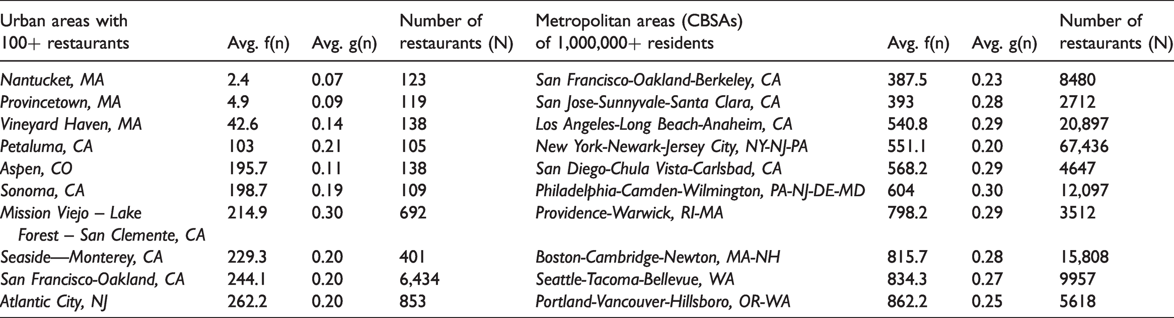
Small cities comprise many of the highest and lowest concentrations of chain and independent restaurants. Nantucket, MA, a wealthy coastal tourist area, has only 7.3% chain restaurants (denoted as average of g(n) of the UA), and nearby Provincetown and Vineyard Haven follow suit. Other tourist destinations, such as towns in California’s Wine Country; Atlantic City, NJ; the ski resort town of Aspen, CO; and wealthy retirement area, Sedona, AZ, also have low chainness rates (Table 2). Vacationing in these spots often requires a baseline amount of disposable income (for lodging, etc.), making expensive restaurants viable. In addition, seasonal restaurants that specialize in local cuisine tend to thrive herein tourist locations. Some tourist areas, such as Carmel, CA, Bristol, RI, and Port Townsend, WA, have even banned chain stores from their downtowns (Bobrowski, 2012). Cities marked with many chain restaurants are found in the South and toward Ohio and Kentucky and contain up to 65% chain restaurants. McCity-inclined foodscapes tend to be small towns and cities in the South and Midwest (Figure 1, see also Table S6).

Table 2.

Top 10 locales with the lowest chainness rates (see Table S6 for top 10 locales with the highest chainness rates).

Urban areas with 100+ restaurants	Avg. f(n)	Avg. g(n)	Number ofrestaurants (N)	Metropolitan areas (CBSAs) of 1,000,000+ residents	Avg. f(n)	Avg. g(n)	Number ofrestaurants (N)
Nantucket, MA	2.4	0.07	123	San Francisco-Oakland-Berkeley, CA	387.5	0.23	8480
Provincetown, MA	4.9	0.09	119	San Jose-Sunnyvale-Santa Clara, CA	393	0.28	2712
Vineyard Haven, MA	42.6	0.14	138	Los Angeles-Long Beach-Anaheim, CA	540.8	0.29	20,897
Petaluma, CA	103	0.21	105	New York-Newark-Jersey City, NY-NJ-PA	551.1	0.20	67,436
Aspen, CO	195.7	0.11	138	San Diego-Chula Vista-Carlsbad, CA	568.2	0.29	4647
Sonoma, CA	198.7	0.19	109	Philadelphia-Camden-Wilmington, PA-NJ-DE-MD	604	0.30	12,097
Mission Viejo – Lake Forest – San Clemente, CA	214.9	0.30	692	Providence-Warwick, RI-MA	798.2	0.29	3512
Seaside—Monterey, CA	229.3	0.20	401	Boston-Cambridge-Newton, MA-NH	815.7	0.28	15,808
San Francisco-Oakland, CA	244.1	0.20	6,434	Seattle-Tacoma-Bellevue, WA	834.3	0.27	9957
Atlantic City, NJ	262.2	0.20	853	Portland-Vancouver-Hillsboro, OR-WA	862.2	0.25	5618

Figure 1.

(Left) Average percentage of chain restaurants (average of (g(n)) in major U.S. urbanized areas and urban clusters (U.S. Census Bureau, 2019). Coastal regions have fewer chain restaurants than inland counterparts. Small towns in the U.S. Midwest and South have the highest concentration of chain restaurants. (Right) Average percentage chain values by CBSA range from 11% to 72%. Places with high chainness follow interstate highways and proliferate in the Midwest and South (see Figure S4 for f(n) by CBSA).

Figure 2.

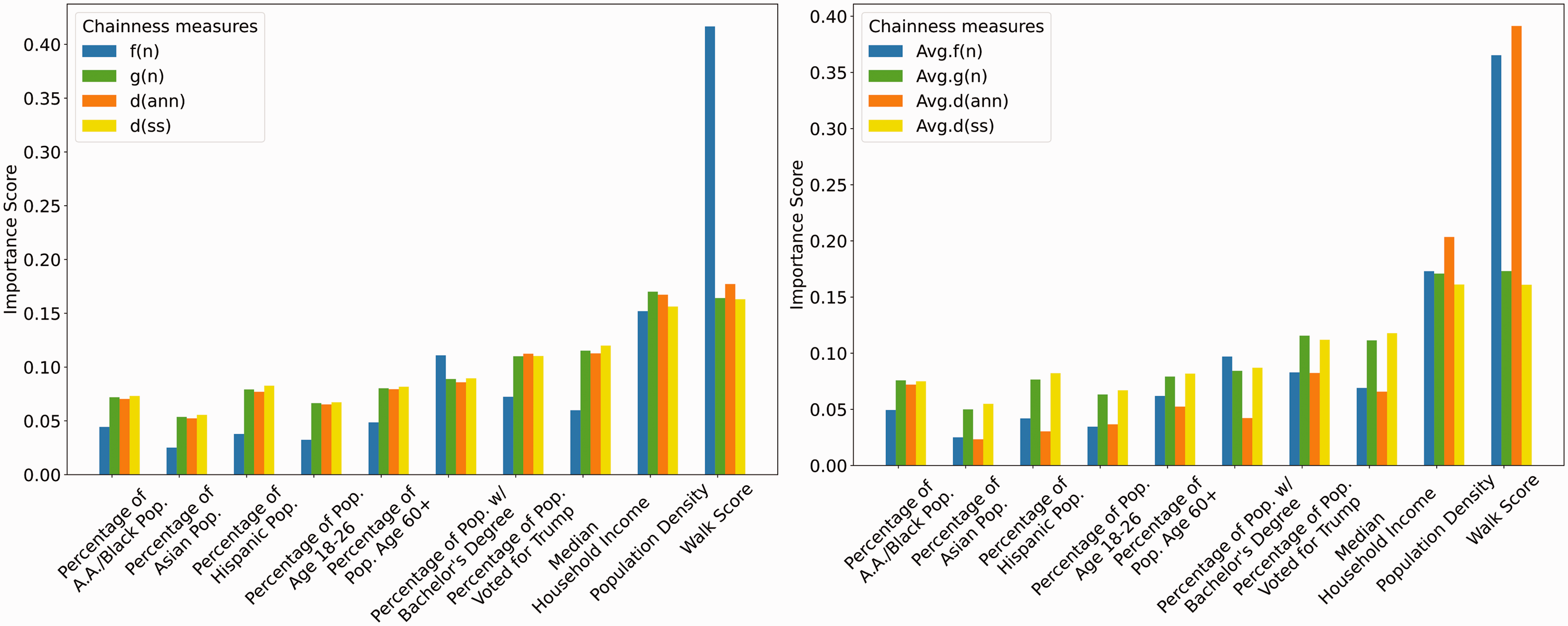
The random forest models output an importance score for each place characteristic, which represents the place characteristic’s ability to distinguish restaurants with high or low chainness. At left are results at the point level, at right, the census tract level. A.A.: African American.

The percent of chains (g(n)) and restaurant replicability (f(n)) at the CBSA level also exhibit similar regional trends. Coastal metropolitan areas such as New York (lowest in percent chain) and San Francisco (lowest in replicability) tend to have low chainness. In contrast, cities in the South (e.g., Nashville), Midwest (e.g., Indianapolis), or Southwest (e.g., Phoenix) are more subject to chains.

Random Forest models at the point and census tract level

According to the random forest results, walkability (i.e. Walk Score), population density, median household income, and the percentage of voters for Trump in 2016 are the top four factors in predicting chainness. In particular, Walk Score is very informative of restaurant frequency f(n) at both the point and census tract level. Among the four, population density and votes for Trump moderately correlate with walkability (Pearson’s r is 0.59 and –0.57, respectively), while median household income has only minimal correlation with either variables, indicating a separate pathway to predict chainness. Race, age, and education attainment contribute less to the random forest prediction.

We use PDPs to illustrate the influence of socioeconomic variables on the predicted chainness measures (see Figure 3). Results at the point and census tract levels are very similar. Areas with very low or very high Walk Score, population density, and median household income tend to have medium or low chainness, and thus maintain a locally run food scene. These areas may correspond to rural tracts or wealthy downtowns. In particular, areas with high Walk Score, such as pedestrian-friendly main streets or tourist areas, have the lowest predicted chainness across all sociodemographic features. Medium-density census tracts (i.e. 1000–4500 people per square mile) that are car-dependent (Walk Score 15 to 40) and have a medium household income (∼$50,000) are most likely to be McCities. Places with higher percentages of college-educated residents (∼40% population) exhibit low levels of chainness (see Figures S6, S7 and Tables S9, S10 for threshold values).

Figure 3.

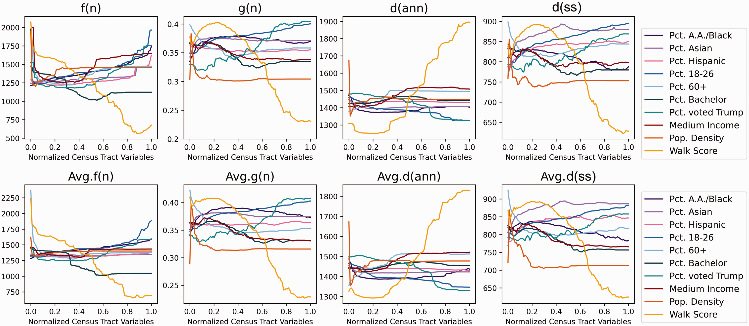
Partial dependence plots (PDPs) show how predicted chainness measures change with the normalized values of socioeconomic variables on the point and census tract level. Top-row plots show results at the point level, and at bottom, the census tract level. A.A.: African American. (See also Figures S5, S6, and Tables S8, S9.)

The predicted chainness measures based on the percentages of non-white population vary by chainness metric (see Figure 3), but this effect may be masked by the long-tail distribution of these variables (e.g., only 23 tracts have more than 80% Asian). Triangulated with quantile plots, T-tests, and a dynamic visualization tool (see Figures S6, S7, S8), we observed that urban niches dominated by white, Asian, Hispanic, mixed racial minority, or elderly (e.g., retirement communities) tend to have low chainness rates.

Areas with concentrations of Trump voters (2016) or college-age students attract chain restaurants. The increase of chainness becomes more drastic when the percentage of Trump voters reaches 50% or when distinctive college towns emerge (e.g., have more than 60% population between 18 and 26 years old) (see Figure 3 and Figure S5), as found in McLean-Meyinsse et al. (2015). Areas with a high percentage of Black residents show increased f(n), but decreased chainness in g(n), d(ann), and d(ss), which may be explained by a mixed pattern of national chains and independent restaurants in these neighborhoods, or regional chains.

OLS regression at the UA level

Consistent with the random forest results, Walk Score is associated with low chainness in the OLS regression (UA and CBSA level) (see Table 3 and Table S10). Chain restaurants tend to be more commonplace in less walkable cities, following findings on the nexus of chain restaurants and car culture (Belasco, 1979). OLS regression predicts that raising the Walk Score value by 10 units decreases restaurant replicability f(n) by 109 and percent chain g(n) by 4% (Table 3). Increases in median household income, education attainment, and the percentage of elderly resulted in reduced chainness across the four measures. Population density is not significant at the UA level, likely due to sustained high density within UAs.

Table 3.

OLS regression with sociodemographic variables and chainness measures.

	Dependent variables
	Avg. f(n)	Avg. g(n) (%)	Avg. d(ann) (mi)	Avg. d(ss) (mi)
Pct. of Pop. Age 60+ (10%)	–231.6 (36.1)***	–6.8 (0.8)***	181.1 (19.8)**	–85.3 (13.9)***
Pct. Pop. w/ Bachelor’s Degree (10%)	–176.6 (30.61)***	–2.3 (0.7)***	46.7 (16.8)***	–64.5 (11.8)***
Walk Score (10)	–109.1 (18.5)***	–3.6 (0.4)***	80.1 (10.1)***	–29.5 (7.1) ***
Median Income ($10,000)	–65.3 (18.3)***	–1.2 (0.4)**	25.1 (10.0)*	–3.9 (7.0)***
Pop. Density (1000 per mi²)	4.1 (9.2)	0.2 (0.2)	–1.7 (5.0)	–5.0 (3.5)
Pct. Asian Pop. (10%)	–44.1 (52.6)	2.4 (1.1)*	–64.9 (28.8)*	88.5 (20.2) ***
Pct. Hispanic Pop. (10%)	–55.9 (10.3)***	–0.2 (0.2)	3.6 (5.6)	12.3 (4.0) **
Pct. Pop. Age 18–26 (10%)	–17.7 (27.1)	0.6 (0.6)	–18.8 (14.8)	14.7 (10.4)
Pct. African American/Black Pop. (10%)	6.4 (12.8)	1.2 (0.3)***	–27.3 (7.0)***	0.8 (4.9)
Pct. Pop. Voted Trump (10%)	52.9 (12.9)***	1.9 (0.3)***	–51.3 (7.1)***	18.1 (4.98)***
Observation	671	671	671	671
R²	0.503	0.529	0.501	0.349
Adjusted R²	0.495	0.522	0.493	0.339

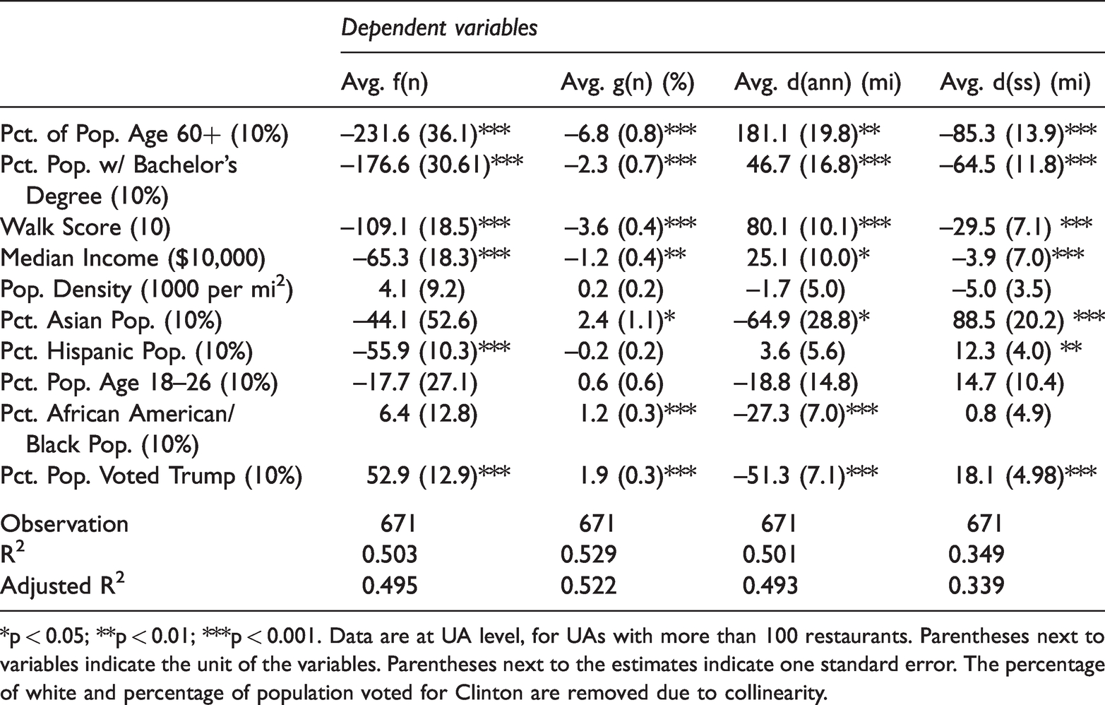
*p < 0.05; **p < 0.01; ***p < 0.001. Data are at UA level, for UAs with more than 100 restaurants. Parentheses next to variables indicate the unit of the variables. Parentheses next to the estimates indicate one standard error. The percentage of white and percentage of population voted for Clinton are removed due to collinearity.

The percentage of Trump voters is still the most indicative factor in defining a McCity, i.e. an area with high chainness, across spatial scales (census tracts, UA, or CBSA), even after controlling for race, age, income, and education (Table 3 and Table S10). The percentage of college-aged individuals does not correlate with chainness, but a concentration of young people, inferring college campuses, has higher chainness.

Race has inconclusive correlation with the chainness of a city as the statistical significance varies based on metric definition. For example, the OLS regression at UA level indicates that a higher percentage of Hispanic population will decrease replicability but increase spatial span. This inconsistency may come from the tendency for ethnic chain restaurants to expand in patches of ethnic neighborhoods that are not distributed evenly in geographic space or the fact that the Hispanic population may live in sparser areas.

Analysis by Restaurant Location

Thus far, we have largely examined the correlation of chainness with variables related to the population. However, the presence of water vistas and highway proliferation are also likely to drive chainness, as the former represents coveted commercial real estate and landscape experience, and the latter is a known covariate with fast food. We found that chain restaurants are more likely to locate close to interstate highway ramps, while independent restaurants are near water bodies and nearby coastlines. Seventy eight percent of restaurants near the water (less than or equal to zero meters) are independent, and the replicability (avg f(n)) is significantly less than those in the 900–1000 meter range.² Although highway and water bodies’ respective averages appear quite different (avg f(n) is 1000 vs. 1700) at 400 meters, T-tests show that avg f(n) of the restaurants are indistinguishable after 400 meters distance to highways and water bodies (see Figure S9). However, the replicability near the coastline continues to stay low beyond 1000 meters and is lower than the replicability of areas by the water bodies, indicating that coastal cities are attractive for independent restaurants for reasons beyond immediate ambiance of dining on the water.

Discussion and conclusion

This study tied the theoretical concept of “placelessness” to U.S. cities and neighborhoods by examining the location of chain vs. independent restaurants at multiple demographic and spatial scales. We outlined the locations demarcated with local restaurant decisions vs. decisions from large, distant corporations. We defined four different measures for restaurant chainness and conducted random forest and OLS linear regression to reveal which independent variables noted as influential in the literature correlated with high or low chainness.

We found that higher walkability, median income, education attainment, and percentage of elderly correlate with a unique foodscape. Within neighborhoods, dense urban cores and sociodemographic enclaves concentrated with majority white, Asian, Hispanic populations or racial diversity also host more independent restaurants. The seemingly contradictory result is due to simultaneous effects of low chainness in predominantly white retirement resorts and tourist areas, as well as ethnic enclaves. Nearness to coastlines and water bodies and distance from interstate highway ramps were also popular environments for individually run venues. We also found that U.S. Midwest, Great Plains, and the South have high chainness rates. It is notable that only 30% of census tracts and 33% of urban areas have more independent restaurants than chains (g(n) < 0.5), which speaks to “the death of American main street”, a provocative statement supported by a recent study (Talen and Jeong, 2019a).

This analysis can be used to foster an authentic landscape by promoting individual ownership of restaurants. Recommendations from the literature include the construction of a “sweet spot” of popular chains and smaller venues, as a mix of large and small successful businesses drives urban validity and uniqueness (Montgomery, 1998). While we did not test for causality in this work, the creation of mix-used and walkable projects along geographic features such as water bodies and coastlines may invite independent restaurants, and can attract both the creative class and tourists that favor unique landscapes (Florida, 2002). Policy makers can also encourage local entrepreneurs to create diverse and affordable food choices, and support mobile solutions (e.g., food trucks) that serve the high chainness communities (e.g., low-income neighborhoods, college campuses).

Our results also raised concerns about the politics of food choices. Inland cities in U.S. Midwest and South are more likely to be saturated with chain restaurants than their coastal counterparts. The percentage of the population voted to Trump (or Clinton) is the most consistent and significant indicator at predicting more (or less) chain restaurants at a locale. Little evidence is found directly linking conservative notions to chains, but industry reports found that Republican voters tend to patronize pizza chains; pizza chains are in turn notable donors to Republican campaigns (Martin, 2015; Krugman, 2015, Piacenza, 2018). Although political votes do not directly impact the decisions of restaurants opening, the values beyond the votes (i.e., attitudes on traditions, immigrants, etc.) and the sociodemographic groups representative in either camp (i.e., working-class for Trump) may drive the correlation. Seemingly unpolitical food choices can reveal people’s local vs. cosmopolitan orientation and whom they feel connected (through restaurant patronage) (Vavreck, 2020). Measuring the chainness of the landscape can provide information regarding how political and world outlooks influence geographic food choices.

We acknowledge that chainness can be very contextual: its value depends on the geographic unit of analysis used and definition of chainness. The statistics produced are sensitive to the scope and spatial scale used to capture the point patterns of restaurants. For example, a restaurant chain may seem sparsely located within a region (e.g., a large d(ann)), but clustered in the scope of the whole country (e.g., a small d(ss)). Even when paired, these statistics obfuscate the actual point pattern, which we encourage readers to investigate on the interactive map (https://doi.org/10.6084/m9.figshare.14675691 and see SI for screen captures).

We also did not measure whether independent restaurants spatially cluster with other independent restaurants, in general, as our approach highlighted each entity (restaurant name) as the major unit of analysis. In addition, our dataset did not include the location of food trucks, and the data may not be updated frequently, thus altering results. We also did not account for zoning regulations that prohibit chain restaurants.

Future research should address the extent to which chain venues have grown over time, and whether chains have taken the place of independent venues or of other chain venues. Research should also address public demand for chain restaurants. For example, a 2008 ban on fast food in the southern areas of Los Angeles (which had high obesity rates) was not met with widespread public approval (Sturm and Cohen, 2009), suggesting that chain restaurants can be a valued part of the local landscape.

The methodology used here can be also extended to address the issue of chain hotels vs. Airbnb and private hotels, and large retail outlets vs. smaller boutiques. This method can help us better link the costs of placelessness and loss, and benefits of unique landscapes, to actual case studies in the built environment.

COVID-19 note

Recently, the COVID-19 pandemic has left many to mourn the experience of dining out, and due to lack of customers, a number of independent restaurants may not survive the challenges faced with largescale dine-in closures (SafeGraph, 2020). This predicament is especially disheartening as restaurants that continued to provide indoor dining during the pandemic contributed to the spreading of COVID-19 significantly more than any other type of POI (Chang et al. 2021). As restaurants begin to open during safer conditions, the chainness metrics described here can be used to point customers to locales and restaurants under local ownership.

Supplemental Material

sj-pdf-1-epb-10.1177_23998083211014896 - Supplemental material for Measuring McCities: Landscapes of chain and independent restaurants in the United States

Supplemental material, sj-pdf-1-epb-10.1177_23998083211014896 for Measuring McCities: Landscapes of chain and independent restaurants in the United States by Xiaofan Liang and Clio Andris in Environment and Planning B: Urban Analytics and City Science

Footnotes

Acknowledgement

We thank Sorhab Rahimi for assistance with data gathering and suggestions for literature.

Notes

Xiaofan Liang is a PhD student of the School of City and Regional Planning at the Georgia Institute of Technology. She studies urban spatial and social networks and how to make cities a more equitable, livable, and connected.

Clio Andris is an assistant professor in the School of City & Regional Planning and the School of Interactive Computing at the Georgia Institute of Technology.

References

Arefi

(1999) Non-place and placelessness as narratives of loss: Rethinking the notion of place. Journal of Urban Design 4(2): 179–193.

Austin

Melly

Sanchez

, et al. (2005) Clustering of fast-food restaurants around schools: A novel application of spatial statistics to the study of food environments. American Journal of Public Health 95(9): 1575–1581.

Beaulac

Kristjansson

Cummins

(2009) A systematic review of food deserts. Preventing Chronic Disease. Preventing Chronic Disease 6(3): A105.

Belasco

(1979) Toward a culinary common denominator: The rise of Howard Johnson’s, 1925–1940. The Journal of American Culture 2(3): 503–518.

Bergstra

Bengio

(2012) Random search for hyper-parameter optimization. Journal of Machine Learning Research 13(2): 281–305.

Block

Scribner

Desalvo

(2004) Fast food, race/ethnicity, and income: A geographic analysis. American Journal of Preventive Medicine 27(3): 211–217.

Bobrowski

(2012) The regulation of formula businesses and the dormant commerce clause doctrine. The Urban Lawyer 44(1): 227–264.

Bocock

(2008) Consumption. London: Routledge.

Bowman

Gortmaker

Ebbeling

, et al. (2004) Effects of fast-food consumption on energy intake and diet quality among children in a national household survey. Pediatrics 113(1): 112–118.

10.

Bridge

Dowling

(2001) Microgeographies of retailing and gentrification. Australian Geographer 32(1): 93–107.

11.

Brown

(1993) Retail location theory: Evolution and evaluation. The International Review of Retail, Distribution and Consumer Research 3(2): 185–229.

12.

Buttimer

(1980) Home, reach, and the sense of place. In: Seamon

Buttimer

(eds) The Human Experience of Place and Space. Kent, UK: Croom Helm Publishers.

13.

Carroll

Torfason

(2011) Restaurant organizational forms and community in the U.S. in 2005. City & Community 10(1): 1–24.

14.

Chang

Pierson

Koh

, et al. (2021) Mobility network models of COVID-19 explain inequities and inform reopening. Nature 589: 82–87.

15.

Cohen

(1988) Authenticity and commoditization in tourism. Annals of Tourism Research 15(3): 371–386.

16.

Credit

Mack

(2017) Place-making and performance: The impact of walkable built environments on business performance in Phoenix and Boston. Environment and Planning B: Urban Analytics and City Science 46(2): 264–285.

17.

Deng

Newsam

(2017) Quantitative comparison of open-source data for fine-grain mapping of land use. In: Proceedings of the 3rd ACM SIGSPATIAL Workshop on Smart Cities and Urban Analytics (pp. 1-8). New York: Association for Computing Machinery.

18.

Dong

Ratti

Zheng

(2019) Predicting neighborhoods’ socioeconomic attributes using restaurant data. Proceedings of the National Academy of Sciences of the United States of America 116(31): 15447–15452.

19.

Duncan

Aldstadt

Whalen

, et al. (2011) Validation of Walk Score® for estimating neighborhood walkability: An analysis of four US metropolitan areas. International Journal of Environmental Research and Public Health 8(11): 4160–4179.

20.

Featherstone

(2007) Consumer Culture and Postmodernism Theories of Consumer Culture. London: SAGE Publications.

21.

Florida

(2002) Rise of the Creative Class and How it's Transforming Work, Leisure, Community, and Everyday Life. New York: Basic Books.

22.

Frederick

Saguy

Gruys

(2016) Culture, health, and bigotry: How exposure to cultural accounts of fatness shape attitudes about health risk, health policies, and weight-based prejudice. Social Science & Medicine 165: 271–279.

23.

Glaeser

Kim

Luca

(2017) Nowcasting the local economy: Using Yelp data to measure economic activity. National Bureau of Economic Research. Working Paper No. w24010.

24.

Harvey

(1993) From space to place and back again: Reflections on the condition of postmodernity. In: Bird

Curtis

, and Tickner

(eds) Mapping the Futures. London: Routledge, pp. 17–44.

25.

Hurvitz

Moudon

Rehm

, et al. (2009) Arterial roads and area socioeconomic status are predictors of fast food restaurant density in King County, WA. International Journal of Behavioral Nutrition and Physical Activity 6(1): 46.

26.

Jones

Ram

Abbas

(2004) Ethnic minority enterprise in an inner-city context: The case of the independent restaurant sector in Birmingham. In: Parkinson

Boddy

(eds) City Matters: Competitiveness, Cohesion and Urban Governance. Bristol, UK: Policy Press, pp. 307–322.

27.

Jones

Al-Shaheen

Dunse

(2016) Anatomy of a successful high street shopping Centre. Journal of Urban Design 21(4): 495–511.

28.

Karsten

Kamphuis

Remeijnse

(2015) ‘Time-out’ with the family: The shaping of family leisure in the new urban consumption spaces of cafes, bars and restaurants. Leisure Studies 34(2): 166–181.

29.

Kersh

(2009) The politics of obesity: A current assessment and look ahead. Milbank Quarterly 87(1): 295–316.

30.

Koschinsky

Talen

Alfonzo

, et al. (2017) How walkable is walker’s paradise? Environment and Planning B: Urban Analytics and City Science 44(2): 343–363.

31.

Kruft

H-W

(1994) History of Architectural Theory. Hudson, NY: Princeton Architectural Press.

32.

Krugman P (2015) Pepperoni turns partisan. Available at: https://www.nytimes.com/2015/03/06/opinion/paul-krugman-pepperoni-turns-partisan.html (accessed 31 May 2020).

33.

Kunstler

(1994) Geography of Nowhere: The Rise and Decline of America’s man-made landscape. New York: Simon and Schuster.

34.

Kwate

NOA

Yau

Loh

, et al. (2009) Inequality in obesigenic environments: Fast food density in New York City. Health & Place 15(1): 364–373.

35.

Lash

Urry

(1993) Economies of Signs and Space. London: SAGE Publications.

36.

Lees

Slater

Wyly

(2013) Gentrification. London: Routledge.

37.

Leslie

Frankenfeld

Makara

(2012) The spatial food environment of the DC metropolitan area: Clustering, co-location, and categorical differentiation. Applied Geography 35(1–2): 300–307.

38.

Liaw

Wiener

(2002) Classification and regression by randomForest. R News 2(3): 18–22.

39.

Lopez

Hynes

(2003) Sprawl in the 1990s: Measurement, distribution, and trends. Urban Affairs Review 38(3): 325–355.

40.

Martin A (2015) Inside the powerful lobby fighting for your right to eat pizza. Available at: https://www.bloomberg.com/news/features/2015-03-03/junk-food-s-last-stand-the-pizza-lobby-is-not-backing-down (accessed 31 May 2020).

41.

McLean-Meyinsse

Taylor

Gager

(2015) Self-reported consumption of fast-food meals by university students. Journal of Food Distribution Research 46: 1–7.

42.

Melaniphy

(1992) Restaurant and Fast Food Site Selection. New Jersey: John Wiley.

43.

Miller

(1995) Acknowledging Consumption: A Review of New Studies. London: Routledge.

44.

Milligan

(1998) Interactional past and potential: The social construction of place attachment. Symbolic Interaction 21(1): 1–33.

45.

MIT Election Data and Science Lab (2018) U.S. President Precinct-Level Returns (2016). Available at: https://dataverse.harvard.edu/dataset.xhtml?persistentId=doi:10.7910/DVN/LYWX3D (accessed 31 May 2020).

46.

Montgomery

(1998) Making a city: Urbanity, vitality and urban design. Journal of Urban Design 3(1): 93–116.

47.

Morland

Wing

Diez Roux

, et al. (2002) Neighborhood characteristics associated with the location of food stores and food service places. American Journal of Preventive Medicine 22(1): 23–29.

48.

Moro

(2019) The Atlas of Inequality. Available at: https://inequality.media.mit.edu/ (accessed 31 May 2020).

49.

Mossberg

Eide

(2017) Storytelling and meal experience concepts. European Planning Studies 25(7): 1184–1199.

50.

Mullins

Natalier

Smith

, et al. (1999) Cities and consumption spaces. Urban Affairs Review 35(1): 44–71.

51.

Nezhad

Eshrati

(2015) A definition of authenticity concept in conservation of cultural landscapes. International Journal of Architectural Research: Archnet-IJAR 9(1): 93–107.

52.

Onesti A (2017) Built environment, creativity, social art: The recovery of public space as engine of human development. Region: the journal of ERSA 4(3): 87–118.

53.

Piacenza

(2018) Partisan divide: Why pizza chains are more popular among republicans. Morning Consult. Available at: https://morningconsult.com/2018/01/25/partisan-divide-why-pizza-chains-are-more-popular-among-republicans/ (accessed 31 May 2020).

54.

Pine

Gilmore

(1998) Welcome to the experience economy. Harvard Business Review 76(4): 97–105.

55.

Piramanayagam

Sud

Seal

(2020) Relationship between tourists’ local food experiencescape, satisfaction and behavioural intention. Anatolia 31(2): 316–330.

56.

Relph

(1976) Place and Placelessness. London: Pion.

57.

Rivlin

(1982) Group membership and place meanings in an urban neighborhood. Journal of Social Issues 38(3): 75–93.

58.

Rosenbaum

(2006) Exploring the social supportive role of third places in consumers’ lives. Journal of Service Research 9(1): 59–72.

59.

SafeGraph (2020) U.S. consumer activity during COVID-19 pandemic. Available at: www.safegraph.com/dashboard/covid19-commerce-patterns (accessed 31 May 2020).

60.

Sands

Oppewal

Beverland

(2015) How in-store educational and entertaining events influence shopper satisfaction. Journal of Retailing and Consumer Services 23: 9–20.

61.

Scannell

Gifford

(2010) Defining place attachment: A tripartite organizing framework. Journal of Environmental Psychology 30(1): 1–10.

62.

Sharpley

(1994) Tourism, Tourists and Society. Huntingdon, UK: Elm Publications.

63.

Shoup

(2005) The High Cost of Free Parking. Chicago: Planners Press, American Planning Association.

64.

Shumaker

Taylor

(1983) Toward a clarification of people-place relationship: A model of attachment to place. In: Geller

Feimer

(eds) Environmental Psychology. Directions and Perspectives. London: SAGE Publications, p. 12571.

65.

Sims

(2009) Food, place and authenticity: Local food and the sustainable tourism experience. Journal of Sustainable Tourism 17(3): 321–336.

66.

Small

(2017) How fast food concerned the urban market. Available at: www.citylab.com/life/2017/03/how-fast-food-chains-cornered-the-urban-market/521148/ (accessed 31 May 2020).

67.

Strobl

Boulesteix

Zeileis

, et al. (2007) Bias in random forest variable importance measures: Illustrations, sources and a solution. BMC Bioinformatics 8(1): 25.

68.

Sturm

Cohen

(2009) Zoning for health? The year-old ban on new fast-food restaurants in South LA: The ordinance isn’t a promising approach to attacking obesity. Health Affairs 28(6): 1088–1097.

69.

Talen

Jeong

(2019) Does the classic American main street still exist? An exploratory look. Journal of Urban Design 24(1): 78–98.

70.

Talen

Jeong

(2019) What is the value of ‘main street’? Framing and testing the arguments. Cities 92: 208–218.

71.

Teixeira

Palmeira

Branco

, et al. (2004) Who will lose weight? A reexamination of predictors of weight loss in women. International Journal of Behavioral Nutrition and Physical Activity 1: 12.

72.

The NPD Group (2018) Total U.S. restaurant count reaches 647,288, a drop from last year due to decline in independent restaurant units, Reports NPD. Available at: www.prweb.com/releases/2018/02/prweb15204703.htm (accessed 31 May 2020).

73.

Trubek

(2008) The Taste of Place. Berkeley, CA: University of California Press.

74.

U.S. Census Bureau (2019) TIGER/line shapefiles. Available at: www.census.gov/geographies/mapping-files/time-series/geo/tiger-line-file.html (accessed 1 June 2020).

75.

Vavreck

(2020) Bernie Sanders, and how Indian food can predict vote choice. Available at: www.nytimes.com/2020/01/30/upshot/bernie-sanders-indian-food.html (accessed 31 May 2020).

76.

Wasfi

Dasgupta

Eluru

, et al. (2016) Exposure to walkable neighbourhoods in urban areas increases utilitarian walking: Longitudinal study of Canadians. Journal of Transport & Health 3(4): 440–447.

77.

Walk Score (n.d.) Walk Score Methodology. Available at: www.walkscore.com/methodology.shtml (accessed 1 June 2020).

78.

Webber

(1964) The urban place and the nonplace urban realm. In: Webber

(ed) Explorations into Urban Structure. Philadelphia, PA: University of Pennsylvania Press, pp. 79–153.

79.

Yang

Diez-Roux

(2012) Walking distance by trip purpose and population subgroups. American Journal of Preventive Medicine 43(1): 11–19.

80.

Zeng

Zhao

Sun

(2014) Sustainable development mechanism of food culture’s translocal production based on authenticity. Sustainability 6(10): 7030–7047.

81.

Zukin

(1998) Urban lifestyles: Diversity and standardisation in spaces of consumption. Urban Studies 35(5–6): 825–839.

82.

Zukin

(2009) Naked City: The Death and Life of Authentic Urban Places. Oxford, UK: Oxford University Press.

Supplementary Material

Please find the following supplemental material available below.

For Open Access articles published under a Creative Commons License, all supplemental material carries the same license as the article it is associated with.

For non-Open Access articles published, all supplemental material carries a non-exclusive license, and permission requests for re-use of supplemental material or any part of supplemental material shall be sent directly to the copyright owner as specified in the copyright notice associated with the article.

0.00 MB

3.75 MB