Determinants of Urban land development: A panel study for U.S. metropolitan areas

Abstract

This study examines the extent and determinants of urban land expansion and fragmentation for 104 U.S. metropolitan areas for the time period 2001-2019. It leverages temporally and spatially consistent, satellite-based data. The analysis distinguishes among four different intensity levels of urban development and makes use of a number of landscape fragmentation metrics. Estimation relies on two-way fixed-effects panel techniques. Our time fixed-effects indicate that high-intensity urban developments grew by about 25% from 2001 to 2019, low-intensity developments by about 5%. The percentage increases for the corresponding fragmentation statistics are higher, at about 40% and 15%, respectively. Higher gasoline prices are associated with less urban land expansion and fragmentation.

Keywords

Urban land development sprawl U.S. metropolitan areas satellite data panel data estimators

Introduction

This study contributes to the research on the extent and determinants of the spatial size and fragmentation of urban areas that developed with the seminal work on the monocentric city model by Brueckner and Fansler (1983). Our data set covers 104 U.S. metropolitan areas (MSAs) and about ⅔ of the country-wide population at the mid-point of our sample. We leverage newly available, temporally and spatially consistent, satellite-based data (NLCD-2019).¹ Our data set covers 8 years over the time period 2001-2019 for a maximum of 832 year/MSA observations.

Similar to more recent empirical work in this area, such as Deng et al. (2008) for China, Paulsen (2012) for the U.S., as well as Oueslati et al. (2015) and Garcia-López (2019) for Europe, our study goes beyond least squares estimates on cross-section data (e.g., Spivey, 2008) or empirical extensions to multiple-year data sets (e.g., McGrath, 2005). We employ panel data estimators to break some of the main endogeneity issues arising from omitted time-invariant variables. Importantly, we go beyond earlier panel data work with fixed-effects estimators in that we also use time fixed-effects to account for omitted time-varying variables that affect all metro areas.

However, what truly sets our study apart is that we can draw on the NLCD-2019 data set. This allows us to leverage more years, more detail, and better time-consistency than was previously possible for the U.S. We acknowledge that eight years over a time horizon of close to two decades does not even approximate the time horizon of the collaborative project that resulted in the Atlas of Urban Expansion (Angel et al., 2012). However, we cover far more locations for the U.S. (104) than the Atlas (14 in its latest rendition of 2016), and we provide estimates of the economic factors associated with urban land expansion and fragmentation.

Importantly, the NLCD-2019 data allow us to work with four different intensities of urban development, from largely open-space areas to high-intensity developments.² This is a move away from binary urban/rural classifications, which are central to efforts by the U.S. Census Bureau to identify urban areas based on the population density of standard geographical units, such as Census tracts. This binary classification has been used for analyzing the determinants of urban land expansion in numerous studies (e.g., Wassmer, 2006, 2016; Song and Zenou, 2006; Geshkov and DeSalvo, 2012; Paulsen, 2012).

In the spirit of Burchfield et al. (2006), Oueslati et al. (2015), and Garcia-López (2019), our analysis is not confined to studying factors influencing urban land expansion over time. We also examine the change in urban fragmentation associated with urban expansion. For that, we make use of a number of fragmentation metrics with a long history in landscape analysis (McGarigal and Marks,1995). These metrics not only ease replicability, they also have been applied in recent urban sprawl studies and shown to be fully consistent with population-based sprawl measures (Debbage et al., 2017).

Our study goes beyond much of the earlier panel data work in the tradition of the monocentric model in that we consider several less commonly used variables with the potential to improve our understanding of urban land expansion and fragmentation over time. That includes numerous proxies for transportation costs, indicators for the influence of political parties, and the types of buildings (single-family vs. multi-family housing) that receive construction permits.

Related literature

Urban land development is studied in numerous academic fields, including but not limited to economics, real estate, environmental studies, urban and regional planning, and geography. Consistent with this broad interest in land use, the issues addressed in the literature are wide-ranging. They include, for example, methods to better identify changes in land use, the drivers of land use, its consequences, and potential policies to curb or better channel land use. We will limit our brief review to studies on potential determinants of urban land use, which is the focus of our contribution.

Numerous studies analyzed urban growth and sprawl in the aftermath of the seminal study by Brueckner and Fansler (1983). Reviews of the literature up to the early 2000s are provided by Nechyba and Walsh (2004) and by Patacchini and Zenou (2009) for Europe. In the last two decades, the empirical literature on land expansion and sprawl has expanded in terms of both the scope and quality of the data and the sophistication of the estimation techniques. To place our contribution, it is useful to consider a few central guide posts.

One key aspect that differentiates studies on the determinants of urban growth and sprawl is the type of data employed for the dependent variable. Most studies on the U.S. use either the Census definitions of urban areas or data derived from satellite imagery; a few employ both, typically to accommodate data problems (e.g., Burchfield et al., 2006; Paulsen, 2012). Some draw on entirely different data, such as Paulsen (2014), who uses Census data on housing density and related metrics, or Mustafa et al. (2018), who rely on cadastral data on land ownership in the province of Wallonia (Belgium).

Studies based on U.S. Census data rely on the Census definitions of urban areas to measure urban expansion (sprawl). The Census Bureau counts tracts or block groups on the fringes of urban areas as urban as opposed to rural if the population density is above a certain threshold. This binary classification is not directly tied to built-up land or sprawl, but driven by population. Numerous studies use these data to examine whether urban areas respond on their fringes to growth containment policies (e.g., McGrath, 2005; Wassmer, 2006, 2016; Song and Zenou, 2006; Hamidi and Ewing, 2014). One practical issue with these data is that Census updates of urban areas happen only after each decennial census. That significantly limits the number of observations available for study. Another limitation is related to the fact that there are far fewer variables available for urban areas (to explain their changes over time) than for alternative classifications, such as MSAs.

Satellite-based data on urban development can capture changes in built-up land independent of population changes and across the entire space of geographical entities, not just along their fringes. In addition, research is not limited to areas classified by the Census Bureau as urban areas. Satellite-based data can be applied to any geographical entity, including MSAs as, for example, in Debbage et al. (2017) or in this study. In fact, it can be applied to any area of the world, regardless of the sophistication of the local statistical data collection agencies or their willingness to adhere to common standards (e.g., Deng et al., 2008; Oueslati et al., 2015; Ehrlich et al., 2018; Garcia-López, 2019). However, their use to study the driving forces behind urban growth and sprawl tends to be a more recent occurrence.³ What sets our study apart from earlier satellite-based work on the U.S. is our ability to make use of NLCD-2019 data. This new NLCD version is unprecedented in detail, year coverage as well as spatial and temporal consistency. This naturally allows for a wider range of applications than was possible with earlier, more limited NLCD versions (e.g., Burchfield et al., 2006; Paulsen, 2012; Debbage et al., 2017).

Studies on urban growth and sprawl can also be organized along the scope of the analysis. Most studies tend to discuss numerous determinants of sprawl, without a specific focus. The present study also falls into this category. Some studies zero in on a single issue. For example, Garcia-López (2019) looks at the impact of roads on sprawl, Young et al. (2016) at gasoline prices and urban parking costs, Hurst and West (2014) at public transit systems, Song and Zenou (2006) and Wassmer (2016) at property taxes, and Dempsey and Plantinga (2013) at urban growth boundaries. Gielen et al. (2021) examine the connection between sprawl and the local government cost of public services.

A final aspect by which we can distinguish among studies on urban growth and sprawl relates to the estimation methods that are employed. That methods matter has been discussed in numerous papers (e.g., Deng et al., 2008; Paulsen, 2012; Wassmer, 2016; Garcia-López, 2019). By now, it is accepted that the traditional least squares approach on cross-section data is likely subject to endogeneity issues arising, among others, from an omitted variables problem. That extends, in principle, also to those studies that rely on standard least squares in a multi-year data setting (e.g., McGrath, 2005). Instrumental variables estimators, as in Garcia-López (2019), or a treatment-effects approach of the difference-in-differences type Dempsey and Plantinga (2013) offer one solution. But most studies going beyond standard least squares employ panel data estimators, either of the random-effects variety (Oueslati et al., 2015) or the fixed-effects type (e.g., Deng et al., 2008; Paulsen, 2012; Wassmer, 2016). Our study also uses a fixed-effects panel estimator, but with the addition of time fixed-effects to capture U.S.-wide influences and with interaction terms between population and some time-invariant factors to highlight the significant variability across MSAs in responding to population growth.

Data and methodology

Data

Our dependent variables on urban land development and fragmentation (Tables 1 and S10) draw on the 2019 version of the National Land Cover Database (NLCD-2019) of the U.S. Geological Service (USGS). NLCD-2019 provides spatially and temporarily consistent land cover classifications for 8 years between 2001 and 2019.⁴ We combine these data with spatial outlines of 104 MSAs taken from the U.S. Census Bureau’s TIGER/Line shapefiles for the year 2013. Section 1 of the Supplemental Material provides a detailed account.

One important aspect that distinguishes our work from earlier studies on the forces behind urban land expansion and fragmentation (e.g., Paulsen, 2012) is our ability to consider four classes of urban development (Tables 1 and S10). Another aspect is our measurement of sprawl. We follow recent work on the measurement of urban sprawl in the U.S. (Debbage et al., 2017) and employ a number of fragmentation metrics developed originally for the measurement of landscape fragmentation. These can be applied directly to our four urban development classes. As shown in Debbage et al. (2017), they tend to be significantly correlated with population-based sprawl indices.

Tables S1 to S8 provide numerous comparisons across MSAs and time of our measures of urban expansion and fragmentation. That includes rankings of MSAs by growth rates in (a) urban land use (Tables S1 to S3) and (b) fragmentation (Tables S4 to S8). What stands out from these comparisons is that growth in urban land use of the medium- and high-intensity classes was an order of magnitude higher for the 2001-19 period than growth in open-space and low-intensity areas. The increase in fragmentation followed a similar pattern, with growth rates even exceeding those of land use. Section 1 of the Supplemental Material gives more detail.

Table 1 provides definitions of our variables; Table S10 adds more detail on the construction of the dependent variables. Table S11 shows the data sources, and Table S13 provides summary statistics. We include standard variables, such as population, income, and proxies for transportation costs, found in most earlier work on the drivers of urban land expansion and sprawl. However, we also consider variables that are not commonly employed in panel data studies. That includes, for example, pre-existing levels of population density or the percentage of undevelopable land. One would expect in this context that a given population increase generates less land expansion in metro areas that are more densely populated to begin with, given that high population density is not a random occurrence but typically a response to natural or man-made constraints. We capture one of the constraints with our variable Undev, the percentage of undevelopable land. Its construction largely follows (Saiz, 2010) and is discussed in Section 1.3 of the Supplemental Material, with Table S9 showing example data.

Table 1.

Variable definitions.

Variable	Definition
Dependent variables—urban area by development class
open-space	Count of 30 × 30 meter areas (900 m²) of class developed, open-space, by MSA and year
low-dens	Count of 30 × 30 meter areas of class developed, low-intensity
med-dens	Count of 30 × 30 meter areas of class developed, medium-intensity
high-dens	Count of 30 × 30 meter areas of class developed, high-intensity
Dependent variables—fragmentation metrics
Np	Number of patches, by MSA, year, and development class
Pd	Patch density: number of patches per 100 hectares
Ai	Aggregation index: 0 = max. fragmented, 100 = one contiguous area
Clumpy	Clumpiness index: −1 = max. fragmented; 0 = randomly distributed; 1 = one contiguous area
Key independent variables
Pop	Population, total
Income	Per capita personal income per year, in USD
Density	Population-weighted density in 2000, in 000s
Undev	Percentage of undevelopable land, defined as the MSA’s area that is covered by water or is steeper than 5%
Transportation cost
GasPrice	Gasoline price—all grades, annual average; either MSA-specific or state-wide and, if unavailable, region-wide averages allocated to individual MSAs
CommRR	0/1 indicator variable, 1 for the presence of a commuter railroad
HeavyR	0/1 indicator variable, 1 for the presence of a heavy rail system (typically subway)
HybridR	0/1 indicator variable, 1 for the presence of a hybrid rail system
LightR	0/1 indicator variable, 1 for the presence of a light rail system
Business climate
Trif_Rep	0/1 indicator variable; 1 if the Republican Party is in control of the state house, the state senate and the governorship; annual data by state
Trif_Dem	0/1 indicator variable; 1 if the Democratic Party is in control of the state house, the state senate and the governorship; annual data by state
Tax	Average per capita state and local tax burden in 2000, by state, allocated to all MSAs in the state; derived for each state as state and local tax revenue per capita in 2000 divided by per capita personal income in 2000
Industry structure
Employm	Total employment
Union_rep	Percentage of employed wage and salary workers (16 years and older) represented by labor unions; average state data allocated to MSAs in the state
Other
BP_Total	Building permits of new, privately owned housing units
BP_pct_1U	Percentage of building permits for single-family houses (base: all housing building permits)

Notes: More detail on the data is given in Tables S10 and S11; summary statistics are in Tables S12 and S13.

Transportation costs are a fundamental driver of land use in the monocentric city model and gasoline prices are likely a key to understanding urban land expansion and fragmentation in the U.S.⁵ Detailed historical gasoline price data are available only for some of the larger MSAs. That is why we have to allocate average state or regional data to the majority of MSAs. The presence of a rail-based transit system by year and MSA is available for several different types of rail systems (Table S11). Given their high construction costs, there is very little variation by MSA over time. This exacerbates the potential problem of reverse causality, which makes it difficult to attach a causal interpretation to the coefficients. Rail systems tend to lower commuting costs for many outlying areas that would otherwise have been inaccessible to commuters. That can open large swaths of land for potential development and may, therefore, generate above-average land expansion and sprawl. Some recent empirical evidence on a positive impact of light rail systems on built-up land is provided by Hurst and West (2014) and Lee and Sener (2017). By contrast, existing rail systems may induce more dense developments close to existing lines and, therefore, avoid sprawl in outlying areas.

Table 1 contains three variables that are meant to proxy the business climate. We hypothesize that the dominance of either the Republican or the Democratic party in the state government has a distinct impact on land use, with Republican dominance being associated with fewer restrictions and, therefore, more land use and fragmentation and Democratic dominance with less land use. A high tax burden from local and state taxes typically involves high property taxes on real estate. The cross-section results of Song and Zenou (2006) suggest that higher property taxes are associated with less sprawl; the panel data findings of Wassmer (2016) point into the opposite direction. We employ pre-existing tax burden data from 2000 to avoid reverse causality issues.

Employment is included as a separate variable to allow for the fact that population and employment may not change in equal proportions. In particular, we would expect an MSA with an increase in employment relative to population to also show more land use. Although it would be useful to explicitly distinguish among the presence of different industries, assuming that they have different space requirements, missing data for many years and MSAs make that impossible. Instead, we use the percentage of union representation as a proxy for industry structure and its change over time. We consider a decline in union representation to be a good indicator for a reduction in manufacturing employment, which is heavily unionized, and a corresponding increase of employment in the service sector, which has little union representation.

The last two variables in Table 1 allow us to examine the role of housing units in predicting land use. The number of construction permits of new housing units is sometimes used as a proxy for land use (e.g., Bimonte and Stabile, 2017). We also have available the percentage of building permits for single-family homes. As urban sprawl is often epitomized by endless rows of newly built, single-family houses, we suspect that a larger share of these housing units could be a sensible predictor of both land use and fragmentation.

Estimation methodology

To identify the determinants of urban development and fragmentation, we employ the following panel data specification with both unit (MSA) and time fixed-effects, the combination of which is also known as two-way fixed-effects

\ln B_{i t} = α \ln {p o p}_{i t} + γ^{'} X_{i t} + {F E}_{i} + {F E}_{t} + \sum_{k = 1}^{K} β_{k} \ln {p o p}_{i t} \cdot Z_{i k} + ε_{i t} .

(1)

Dependent variable $B_{i t}$ in equation (1) is defined in a number of alternative ways (Table 1) to capture urban land expansion or fragmentation for alternative urban development classes. The variable is measured for MSA i $(i = 1, \dots, 104)$ at 8 different points in time t over the period 2001 to 2019. The pre-fix ln stands for the natural logarithm. The disturbance term is given by $ε_{i t}$ .

Population (pop) is our central driving force. $X_{i t}$ is a vector of time-varying variables that capture other drivers of built-up land, such as gasoline prices. The number of variables contained in $X_{i t}$ is relatively modest compared to pure cross-section studies. This has a simple reason: all variables that vary by MSA i but not over time t drop out of equation (1) as a result of our unit (MSA) fixed-effects specification. Importantly, their impact is not lost; it is summarily absorbed by the unit (MSA) fixed-effects, which are identified by ${F E}_{i}$ in equation (1). The time fixed-effects ( ${F E}_{t}$ ) in equation (1) serve an equally important role. They capture the impact of omitted time-varying variables that affect all urban areas over time, such as changes in U.S. inflation, GDP, or interest rates. For our study of urban development for the U.S. after 2000, the term ${F E}_{t}$ in equation (1) also absorbs the string of financial deregulations and innovations after 2001, which together with an unusually expansionary monetary policy set in motion an unprecedented housing boom. Also absorbed by the time fixed-effects is the impact of the Great Recession following the housing bust and the period of intense monetary easing in its aftermath.

We note that Oueslati et al. (2015) uses a random-effects panel estimator instead of a fixed-effects estimator to make the impact of time-invariant regressors explicit. For our data, a standard Hausman test decidedly rejects the random-effects model in favor of the fixed-effects model. However, we are similarly interested in the impact of time-invariant variables because they allow us to see how urban expansion in a given MSA may deviate systematically from the average change across all urban areas, as predicted by the coefficients $α$ and $γ$ .⁶ To allow for potentially heterogeneous responses across metro areas, we make use of interaction terms between our central driving variable population and the k variables identified by $Z_{k}$ .⁷

The interaction term in equation (1) conditions the impact of population on $Z_{i k}$

\frac{\partial \ln B_{i t}}{\partial \ln {p o p}_{i t}} = α + \sum_{k = 1}^{K} β_{k} \cdot Z_{i k} .

(2)

Equation (2) reveals that the elasticity of urban land expansion/fragmentation (B) with respect to population varies systematically with $Z_{i k}$ ( $k = 1, \dots, K$ ) and the estimated coefficients $β_{k}$ . If Z is a 0/1 indicator variable, the elasticity of B with respect to population is given as

\frac{\partial \ln B_{i t}}{\partial \ln {p o p}_{i t}} = α + \sum_{k = 1}^{K} β_{k}

(3)

for those MSAs for which

Z = 1 .

For MSAs for which

Z = 0

, the elasticity equals

α .

If Z is a continuous variable, the population elasticity can be derived as

\frac{\partial \ln B_{i t}}{\partial \ln {p o p}_{i t}} = α + \sum_{k = 1}^{K} β_{k} {\bar{Z}}_{k}

(4)

where

{\bar{Z}}_{k}

is either the mean value of

Z_{i k}

over all MSAs or the mean value for a particular MSA.

Estimation results

Tables 2 and 3 show two-way panel fixed-effects estimation results (equation (1)) for urban land expansion and urban fragmentation (sprawl), respectively.⁸ Both tables distinguish among 3 aggregated classes of urban development: open-space and low-intensity developments (Columns 1 and 2), medium- and high-intensity developments (Columns 3 and 4), and the sum of all four development classes (Columns 5 and 6). For each of the three aggregated classes we show two model versions, a bare-minimum model with just 4 independent variables and a model with a complete set of determining variables. Individual results for each development class and for two additional metrics of fragmentation are available in Tables S14 to S17.

Table 2.

Panel fixed-effects estimates of 900 m² area counts: aggregated classes of development.

	open-space+low-dens		med-dens+high-dens		Sum of all 4 classes
Variables	(1)	(2)	(3)	(4)	(5)	(6)
ln Pop	0.222***	0.324**	0.991***	0.753***	0.341***	0.417***
ln Pop	(0.027)	(0.159)	(0.061)	(0.225)	(0.029)	(0.142)
ln Income	−0.046**	−0.063**	−0.051	−0.017	−0.051**	−0.071**
ln Income	(0.020)	(0.026)	(0.038)	(0.043)	(0.023)	(0.027)
ln Pop * Density	0.006	0.006	−0.093***	−0.072***	0.015	0.023*
ln Pop * Density	(0.009)	(0.010)	(0.014)	(0.015)	(0.012)	(0.012)
ln Pop * Undev	−0.518***	−0.491***	−0.794***	−0.820***	−0.661***	−0.681***
ln Pop * Undev	(0.110)	(0.114)	(0.240)	(0.228)	(0.138)	(0.136)
ln GasPrice		0.017		−0.128***		−0.017
ln GasPrice		(0.021)		(0.036)		(0.022)
ln Pop * CommRR		0.000		0.000		0.000
ln Pop * CommRR		(0.000)		(0.001)		(0.000)
ln Pop * HeavyR		−0.007		−0.131*		−0.148
ln Pop * HeavyR		(0.102)		(0.073)		(0.101)
ln Pop * HybridR		−0.001**		−0.002		−0.001**
ln Pop * HybridR		(0.000)		(0.001)		(0.000)
ln Pop * LightR		0.001		0.000		0.001
ln Pop * LightR		(0.001)		(0.001)		(0.001)
Trif_Rep		0.004*		0.003		0.003**
Trif_Rep		(0.002)		(0.003)		(0.002)
Trif_Dem		0.000		−0.006*		0.001
Trif_Dem		(0.001)		(0.003)		(0.001)
ln Pop * Tax		−1.666		2.020		−1.658
ln Pop * Tax		(1.639)		(2.022)		(1.429)
ln Employm		0.053		−0.013		0.071
ln Employm		(0.047)		(0.108)		(0.048)
ln Union_rep		−0.001		−0.021*		−0.008*
ln Union_rep		(0.005)		(0.011)		(0.004)
ln BP_pct_1U		0.003		0.018**		0.007*
ln BP_pct_1U		(0.004)		(0.008)		(0.004)
Time fixed-effects
dt_2004	0.005***	0.002	0.024***	0.053***	0.010***	0.015***
dt_2006	0.035***	0.027**	0.072***	0.139***	0.044***	0.056***
dt_2008	0.038***	0.028*	0.104***	0.202***	0.055***	0.074***
dt_2011	0.044***	0.035**	0.119***	0.223***	0.062***	0.086***
dt_2013	0.038***	0.028*	0.142***	0.245***	0.064***	0.087***
dt_2016	0.043***	0.041***	0.164***	0.204***	0.074***	0.088***
dt_2019	0.040***	0.037***	0.198***	0.257***	0.083***	0.100***
LSDV R²	0.9996	0.9997	0.9994	0.9994	0.9997	0.9997
within R²	0.7500	0.7582	0.9567	0.9605	0.9199	0.9281

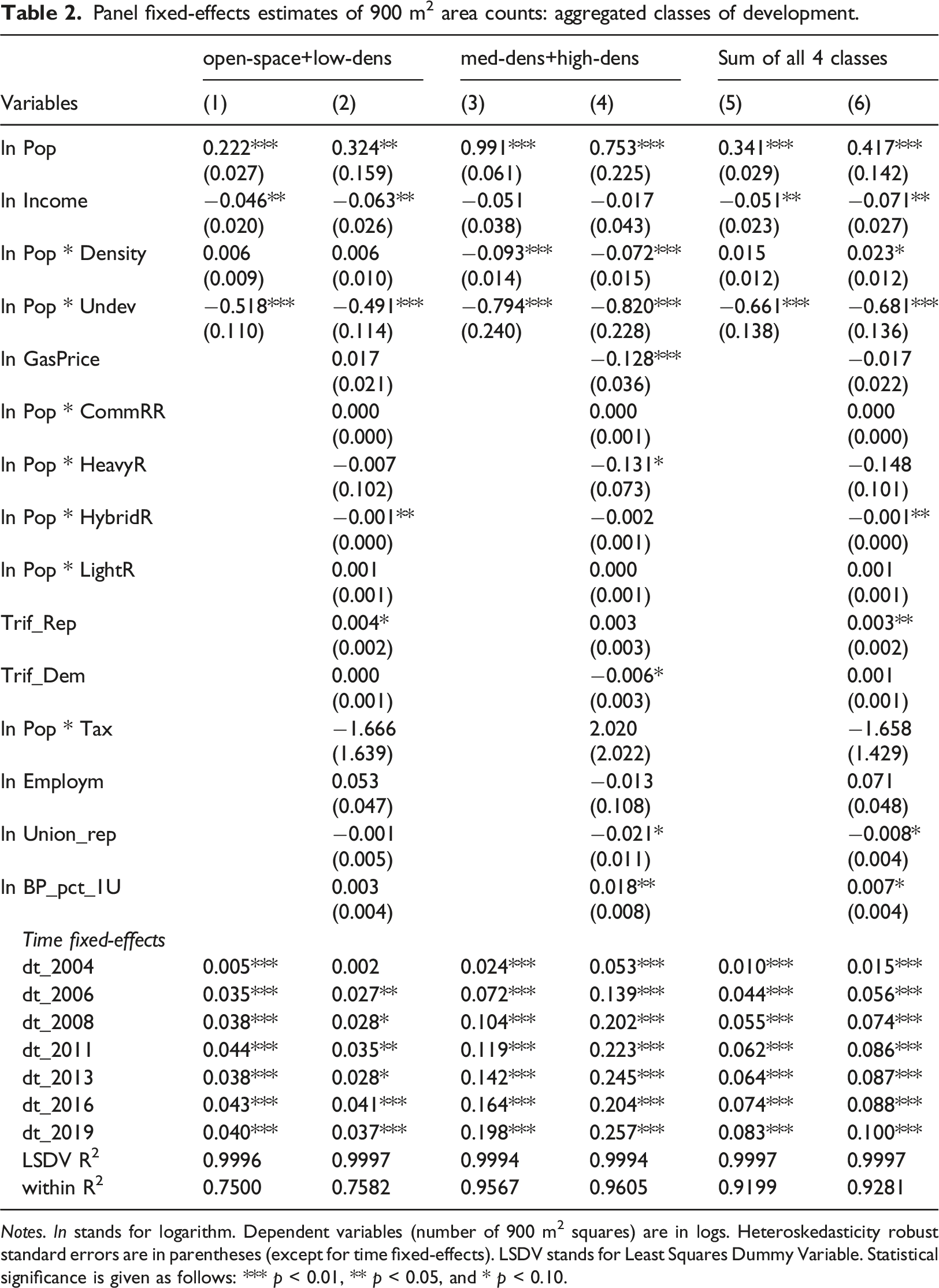
Notes. ln stands for logarithm. Dependent variables (number of 900 m² squares) are in logs. Heteroskedasticity robust standard errors are in parentheses (except for time fixed-effects). LSDV stands for Least Squares Dummy Variable. Statistical significance is given as follows: *** p < 0.01, ** p < 0.05, and * p < 0.10.

Table 3.

Panel fixed-effects estimates of patch counts or density: aggregated classes of development.

Variables	open-space+low-dens		med-dens+high-dens		Sum of all 4 classes
Variables	(1)	(2)	(3)	(4)	(5)	(6)
ln Pop	0.419***	0.925***	1.041***	1.208***	0.515***	0.989***
ln Pop	(0.037)	(0.234)	(0.067)	(0.307)	(0.047)	(0.303)
ln Income	−0.047*	−0.045	−0.014	0.013	−0.044	−0.055
ln Income	(0.028)	(0.032)	(0.038)	(0.047)	(0.033)	(0.036)
ln Pop * Density	−0.015	−0.002	−0.130***	−0.102***	−0.027**	−0.013
ln Pop * Density	(0.011)	(0.011)	(0.014)	(0.013)	(0.013)	(0.013)
ln Pop * Undev	−0.430**	−0.291*	−0.748***	−0.644**	−0.390*	−0.258
ln Pop * Undev	(0.165)	(0.168)	(0.257)	(0.253)	(0.207)	(0.201)
ln GasPrice		−0.086***		−0.138***		−0.112***
ln GasPrice		(0.023)		(0.052)		(0.029)
ln Pop * CommRR		0.000		−0.001		0.000
ln Pop * CommRR		(0.001)		(0.001)		(0.001)
ln Pop * HeavyR		−0.097*		−0.182		−0.135**
ln Pop * HeavyR		(0.050)		(0.117)		(0.054)
ln Pop * HybridR		−0.001***		−0.002*		−0.002***
ln Pop * HybridR		(0.001)		(0.001)		(0.001)
ln Pop * LightR		0.000		−0.001		0.000
ln Pop * LightR		(0.001)		(0.001)		(0.001)
Trif_Rep		0.003		0.008**		0.003
Trif_Rep		(0.002)		(0.004)		(0.002)
Trif_Dem		−0.002		−0.009*		−0.002
Trif_Dem		(0.002)		(0.005)		(0.002)
ln Pop * Tax		−6.404***		−2.865		−6.535**
ln Pop * Tax		(2.393)		(2.901)		(3.069)
ln Employm		0.059		0.011		0.110
ln Employm		(0.066)		(0.112)		(0.074)
ln Union_rep		−0.006		−0.026*		−0.011
ln Union_rep		(0.007)		(0.016)		(0.008)
ln BP_pct_1U		0.006		0.023**		0.011*
ln BP_pct_1U		(0.005)		(0.012)		(0.006)
Time fixed-effects
dt_2004	0.018***	0.040***	0.050***	0.083***	0.025***	0.055***
dt_2006	0.046***	0.095***	0.114***	0.187***	0.061***	0.126***
dt_2008	0.064***	0.135***	0.164***	0.275***	0.086***	0.182***
dt_2011	0.070***	0.150***	0.197***	0.315***	0.099***	0.207***
dt_2013	0.078***	0.157***	0.247***	0.363***	0.117***	0.224***
dt_2016	0.091***	0.127***	0.289***	0.336***	0.138***	0.189***
dt_2019	0.108***	0.158***	0.357***	0.427***	0.169***	0.238***
LSDV R²	0.9994	0.9995	0.9982	0.9984	0.9991	0.9993
within R²	0.9046	0.9187	0.9635	0.9665	0.9378	0.9476

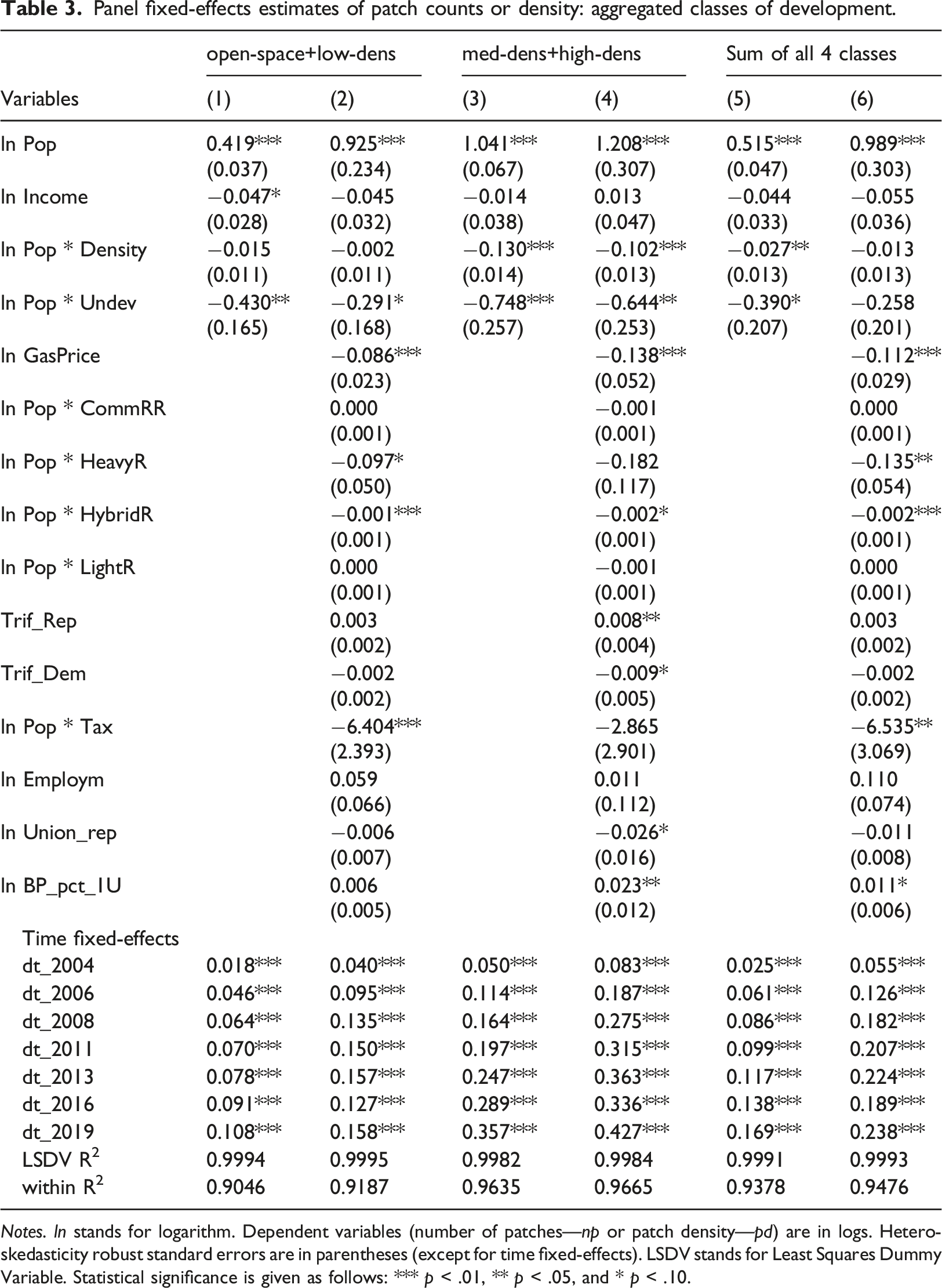
Notes. ln stands for logarithm. Dependent variables (number of patches—np or patch density—pd) are in logs. Heteroskedasticity robust standard errors are in parentheses (except for time fixed-effects). LSDV stands for Least Squares Dummy Variable. Statistical significance is given as follows: *** p < .01, ** p < .05, and * p < .10.

Tables 2 and 3 reveal that including more independent variables than the four given in the bare-minimum model improves the statistical fit, but the gain in explanatory power is small even by the within- $R^{2}$ metric, which measures the fit based on variation over time, the key to the fixed-effects estimator. Similarly, a more complete model has no impact on the coefficient signs and little impact on the statistical significance of the core variables. That changes if one omits the time fixed-effects (Table S18), which are highly significant statistically, both individually and jointly. The explanatory power drops perceptively and the sign and significance of the income variable changes. What also matters for model fit and the behavior of coefficients is the development class that is studied. There are economically meaningful differences between the classes in both Tables 2 and 3 and in the companion Tables S14 to S17.

In discussing the results, it is worthwhile to start with the time fixed-effects. They provide us with an average estimate over all MSAs of the percentage change in urban expansion and fragmentation relative to the base year 2001. According to Table 2, the number of open-space/low-intensity areas increased very little over nearly two decades, by merely 4%, with little to no growth in the last ten years of the sample period. Table S14 shows that all of the growth in this aggregated class was due to growth in the low-density class and none to growth in the open-space class. The growth rates are dramatically higher for the number of medium-/high-intensity areas with an average growth rate of about 25% from 2001 to 2019. Interestingly, most of that growth was accomplished by 2008 during the unprecedented housing boom before the Great Recession. The time fixed-effects of Table 3 show similar dynamics for the fragmentation metric np (pd), but with the difference that the growth rates of fragmentation exceed those of urban expansion by a sizable margin, regardless of the development class. The percentage changes in the fragmentation metrics ai and clumpy (Tables S16 and S17) tend to be far lower.

If one ignores the interaction terms between population and numerous time-invariant variables, our panel data generate an elasticity of urban development with respect to population of 0.28 for the sum of all four development classes (Table S18), with the elasticity being markedly lower at 0.162 for the sum of development classes open-space/low-intensity and significantly higher (0.628) for the medium-/high-intensity classes. The estimates for the sum of the four classes are very similar to those reported in earlier work for the U.S. (Paulsen, 2012). Very comparable values are also result from ordinary least squares (OLS) estimates on percentage differences in all variables between 2001 and 2019 (Table S19).

Our estimates differ from previous work in that our income elasticities tend to be mainly insignificant statistically and negative.⁹ The explanation for this fundamental difference rests with a technical estimation detail: earlier panel data studies of the fixed-effects type did not employ time fixed-effects. If we omit time fixed-effects from our models (Table S18), we can also generate positive income elasticities of a size familiar from earlier work (Paulsen, 2012; Oueslati et al., 2015). However, omitting time fixed-effects would significantly mis-specify our panel data model. We would give up absorbing the impact of numerous time-varying influences on urban development and, thereby, open up the model to endogeneity issues resulting from omitted variables.¹⁰ Tables S14 to S17 suggest that a negative impact of local income on some of the development classes (low-intensity) may translate into more development for other classes (medium-intensity). An explanation for the negative impact of the sum of all four classes (Table 2, Column 6) may lie in the fact that higher local incomes tend to raise the demand for amenities associated with natural surroundings, less noise, and congestion. That may induce residents to try to cut down on additional developments through restrictive zoning regulations and other hurdles (Hilber and Robert-Nicoud, 2013; Gyourko and Molloy, 2015). Future work, both theoretical and empirical, may want to examine this issue in more detail.

The interaction term of population with population density has the expected negative sign only for the medium-/high-intensity aggregate in Columns (3) and (4) of Table 2. The negative coefficient suggests that MSAs with a high pre-existing population density channel their population growth into fewer medium-/high-intensity areas than MSAs with a low population density. Comparing two MSAs with vastly different densities in 2000 provides some intuition on the economic impact of the interaction term. For Miami, with a density of 7.2 in 2000, equation (4) suggests a population elasticity of medium-/high-intensity areas of 0.2346 $(0.753 - 0.072 \cdot 7.2)$ ; for Raleigh, with a density of 1.7 in 2000, the corresponding value is 0.6306 $(0.753 - 0.072 \cdot 1.7) .$ ¹¹ The calculations with equation (4) are analogous for the interaction term of ln Pop and variable Undev, the percentage of undevelopable land. The coefficients of this interaction term are negative and highly significant throughout. The absolute response is highest for the medium-/high-intensity development class. For example, Miami has a value of 0.173 for variable Undev, Raleigh a value of 0.014. According to equation (4), the population elasticity of medium-/high-intensity areas is 0.6111 $(0.753 - 0.820 \cdot 0.173)$ for Miami and 0.7415 $(0.753 - 0.820 \cdot 0.014)$ for Raleigh if one ignores again all other interaction terms with ln Pop. If one combines for both MSAs the coefficients for ln Pop and its interactions with Density and Undev, Miami ends up with a population elasticity for medium-/high-intensity areas of 0.093 $(0.753 - 0.072 \cdot 7.2 - 0.820 \cdot 0.173)$ , Raleigh with 0.619 $(0.753 - 0.072 \cdot 1.7 - 0.820 \cdot 0.014) .$ Miami’s population elasticity turns out to be significantly below the average value of 0.628 derived for the minimalist model in Table S18, while Raleigh’s value deviates little from that average. The calculations for the fragmentation results in Table 3 are analogous and the results are similar.

Transportation costs are a key driver of urban land expansion in the monocentric city model. Tables 2 and 3 reveal the association of five proxies of transportation costs with urban land expansion and fragmentation, respectively. Based on Table 2, a 10% drop in gasoline prices is associated with a 1.3% increase in the number of medium-/high-intensity areas. There is no reaction in the number of open-space/low-intensity areas and no statistically significant response in the sum of all 4 development classes. Table 3 shows an almost identical elasticity for the np (pd) metric and the medium-/high-intensity development class. However, the fragmentation metric for the open-space/low-intensity development class also responds in a sizable and statistically significant manner. That is confirmed in Table S15 for the individual development classes and in Tables S16 and S17 for two alternative metrics of fragmentation, ai and clumpy.¹² Our results broadly conform to those of Young et al. (2016) for Canada. They suggest that gasoline prices may be a potential policy lever to affect both urban expansion and fragmentation.

Of the four interaction terms involving rail systems, heavy rail (subway) and hybrid rail systems appear to moderate the impact of a rising population on both urban expansion (Table 2) and fragmentation (Table 3), while there is no association for commuter and light rail systems. Although the hybrid rail system is almost uniformly statistically significant, the coefficients are too low to be economically meaningful. By contrast, the economic significance for the heavy rail system is noteworthy. Based on equation (3), the existence of such as system lowers the population elasticity by 0.131 for the number of medium-/high-intensity areas (Table 2) and by 0.135 for the number of patches over all four classes of development (Table 3). Coefficients of that size are meaningful, in particular in conjunction with the other interaction terms. For example, Miami’s heavy rail system lowers its predicted population elasticity for medium-/high-intensity areas (Table 2) to effectively zero when combined with its high pre-existing population density and its geographical constraints: $0.753 - 0.072 \cdot 7.2 - 0.820 \cdot 0.173 - 0.131 = - 0.038$ . Tables S14 and S15 suggest that the impact of heavy rail systems is strongly concentrated in the high-intensity development class, both for area counts and fragmentation, with values an order of magnitude larger than those shown in Tables 2 and 3.¹³

Our two proxies for the dominance of either the Republican or the Democratic party have a statistically identifiable impact for both urban expansion (Table 2) and urban fragmentation (Table 3). The coefficients tend to be larger and statistically more significant for the individual development classes in Tables S14 through S17. The coefficient signs are the same for urban expansion and fragmentation. They indicate that a switch to Republican dominance at the state government level is associated with more development and more fragmentation, while a switch to Democratic dominance tends to be associated with the opposite. This supports the results of Williamson (2008). However, little can be said about the direction of causation. Also, the economic relevance is low: urban development or fragmentation change typically by less than 1%.

As a sizable part of the state and local tax burden derives from property taxes on real estate, one would expect to see that locations with a high pre-existing tax burden show less urban expansion as population rises. The interaction term between population and the tax variable is not statistically significant in Table 2. The signs appear to suggest a shift away from open-space/low-intensity areas toward medium-/high-intensity areas. Table S14 clarifies this shift: urban expansion is concentrated in high-intensity areas. The estimation results in Table 3 and Tables S15 through S17 on urban fragmentation reveal that MSAs with a high pre-existing tax burden show less fragmentation, specifically for open-space/low-intensity areas. This result appears to be consistent with the findings of Song and Zenou (2006) but not with those of Wassmer (2016), at least as long as we can assume that property taxes dominate our measure of the state/local tax burden. The association between the tax variable and urban expansion or fragmentation is economically significant. For example, the coefficient of −6.535 in Column (6) of Table 3 implies that an MSA in a state with a high pre-existing average tax burden, say 0.11 as in California, will have its population elasticity cut from 0.989 to 0.27 $(0.989 - 6.535 \cdot 0.11) .$ The drop is less pronounced for a low-tax state, such as Florida, from 0.989 to 0.40 $(0.989 - 6.535 \cdot 0.09) .$ ¹⁴

Employment has a separate positive effect on urban expansion and fragmentation. But that effect is not statistically significant in Tables 2 and 3. The more detailed accounts in the Supplementary Material reveal a statistically significant and economically meaningful elasticity of 0.17 for urban expansion of all development classes in Table S14 and some smaller yet statistically significant elasticities for fragmentation in Table S17. These results suggest an increase in fragmentation (decrease in the clumpy metric) as employment rises for low/medium-intensity areas. The coefficient of the variable representing union representation reveals another aspect of employment, the shifting of jobs out of highly unionized industries, such as manufacturing, toward the much less unionized service sector. The negative signs found throughout Tables 2, 3, S14, S15, and the positive signs in Tables S16 and S17 suggest that less manufacturing is associated with more urban development and more fragmentation. The coefficients are only moderately significant statistically and their economic relevance is low. However, they suggest an interesting aspect of the change out of manufacturing toward services: more space appears to be occupied by the services. Intuitively this makes sense. While manufacturing plants tend to be large on average relative to service locations, they also employment is less spread out, it is more concentrated in a few large plants..

Practitioners in urban planning tend to pay attention to building permits as an indicator of urban expansion. We could not find any meaningful value of that variable in our regressions and, therefore, omit this variable. However, we find an economically small but meaningful association between the share of single-family building permits in all building permits for housing. A higher share of single-family building permits raises both urban development and fragmentation of medium-/high-intensity areas. The results for the fragmentation metrics ai and clumpy in Tables S16 and S17 confirm this tendency, although their responses are not statistically significant.

Section 3 and Tables S20 to S22 of the Supplemental Material provide some sensitivity checks of the results contained in Tables 2 and 3, with an emphasis on potential endogeneity issues. The results of those checks are largely consistent with those discussed above.

Conclusion

We identify sizable differences in urban land expansion and fragmentation for areas with different intensities of development. For the average metropolitan area, our time fixed-effects indicate that medium- and high-intensity urban developments grew by about 25% from 2001 to 2019, more lightly developed areas by much less than 10%. The percentage increases in our fragmentation metrics also reveal larger values for the more intensely developed areas, with the absolute size of these increases varying by the particular metric. The intuitively most straightforward fragmentation measure reveals an increase in fragmentation by 45% from 2001 to 2019 for heavily developed areas, far in excess of that for urban land expansion.

Most of the estimated coefficients tend to be consistent in sign and significance across the urban land expansion and fragmentation metrics. This suggests that one can probably limit the analysis to one or the other without missing key aspects of urban growth. However, the coefficient estimates tend to differ in size and significance, sometimes also in sign, across different intensities of urban land development. Therefore, depending on the purpose of a given study, it may be useful to go beyond highly aggregate measures of urban land development and differentiate by intensity of development.

Population change has an average impact on urban expansion similar to that found in earlier work with panel data on the U.S., with elasticities around 0.3 in the aggregate. For a common fragmentation metric, the elasticity is closer to 0.4. The values are much larger for highly developed areas, at about 0.6, for both urban land expansion and fragmentation. The average results hide significant differences in population elasticities across metro areas; these are tied to pre-existing population densities, geographical constraints, and other time-fixed variables. Contrary to earlier work, we find no positive association between local income changes and urban land development or fragmentation. We show that positive values result from panel data estimators only if one omits time fixed-effects, which capture the influence of U.S.-wide changes over time, such as those associated with the credit and housing boom leading up to the Great Recession or the unprecedented quantitative easing of monetary policy thereafter.

As for policy consequences, our results suggest that higher gasoline prices may lower urban land expansion and fragmentation. As regards future, policy-relevant work on urban land expansion and sprawl, we believe it may be useful to give some thought to an idea advanced by Jaeger and Schwick (2014) and put to use in Switzerland: integrating some of our or other measures of urban land expansion and fragmentation into a usable monitoring framework.

Supplemental Material

Supplemental Material—Determinants of Urban land development: A panel study for U.S. metropolitan areas

Supplemental Material for Determinants of Urban land development: A panel study for U.S. metropolitan areas by Joachim Zietz, Heiko Kirchhain in Environment and Planning B: Urban Analytics and City Science

Footnotes

Acknowledgments

We thank the reviewers for suggesting significant improvements.

Author Contributions

JZ: Additional data procurement, estimation, and writing on initial version; paper revisions.

HK: Conceptualizing idea, data procurement, regressions, and write-up on initial version; literature check, review, and editing of paper revision.

Declaration of conflicting interests

The author(s) declared no potential conflicts of interest with respect to the research, authorship, and/or publication of this article.

Funding

The author(s) received no financial support for the research, authorship, and/or publication of this article.

ORCID iD

Joachim Zietz

Supplemental Material

Supplemental material for this article is available online.

Notes

Author Biographies

Dr. Joachim Zietz is an "ausserplanmaessiger" professor of real estate econometrics at EBS University, Germany, and engaged in supporting the masters and doctoral programs at the university's Real Estate Management Institute (REMI). Up until 2016, he was professor of economics at several US universities. Earlier in his career, he had appointments at the Kiel Institute for the World Economy (Germany) and the International Food Policy Research Institute (IFPRI) in Washington, DC. He is a former editor of the Journal of Economics and Finance and has done consulting for the World Bank, OECD, ILO, FAO, IFPRI and other organisations.

Dr. Heiko Kirchhain is a senior real estate specialist at MEAG, the asset management subsidiary of MunichRE. He holds a PhD in real estate economics from EBS University, completed postgraduate studies in real estate at the University of Regensburg and undergraduate studies in geography at the University of Munich. His areas of expertise are the impact of exogenous shocks on real estate markets, the interactions between automobile production sites and local real estate markets as well as the use of remote sensing as a data collection tool in real estate research.

References

Angel

Parent

Civco

, et al. (2012) Atlas of Urban Expansion. Cambridge, MA: Lincoln Institute of Land Policy.

Bimonte

Stabile

(2017) Land consumption and income in Italy: A Case of inverted EKC. Ecological Economics 131: 36–43.

Brueckner

Fansler

(1983) The economics of urban sprawl: Theory and evidence on the spatial sizes of cities. Review of Economics and Statistics 65(3): 479–482.

Burchfield

Overman

Puga

, et al. (2006) Causes of sprawl: A portrait from space. Quarterly Journal of Economics 121(2): 587–633.

Debbage

Bereitschaft

Shepherd

(2017) Quantifying the spatiotemporal trends of urban sprawl among large US metropolitan areas via spatial metrics. Applied Spatial Analysis and Policy 10(3): 317–345.

Dempsey

Plantinga

(2013) How well do urban growth boundaries contain development? Results for Oregon using a difference-in-difference estimator. Regional Science and Urban Economics 43(6): 996–1007.

Deng

Huang

Rozelle

, et al. (2008) Growth, population and industrialization, and urban land expansion of China. Journal of Urban Economics 63(1): 96–115.

Donaldson

Storeygard

(2016) The view from above: Applications of satellite data in economics. Journal of Economic Perspectives 30(4): 171–198.

Ehrlich

Hilber

Schöni

(2018) Institutional settings and urban sprawl: Evidence from Europe. Journal of Housing Economics 42: 4–18.

10.

Garcia-López

(2019) All roads lead to Rome and to sprawl? Evidence from European cities. Regional Science and Urban Economics 79: 103467.

11.

Gielen

Riutort-Mayol

Miralles i Garcia

, et al. (2021) Cost assessment of urban sprawl on municipal services using hierarchical regression. Environment and Planning B: Urban Analytics and City Science 48(2): 280–297.

12.

Geshkov

DeSalvo

(2012) The effect of land-use controls on the spatial size of U.S. urbanized areas. Journal of Regional Science 52(4): 648–675.

13.

Gyourko

Molloy

(2015) Chapter 19 - Regulation and Housing Supply. In: Duranton

Henderson

Strange

(eds), Handbook of Regional and Urban Economics. Netherland: Elsevier, volume 5, pp. 1289–1337.

14.

Hamidi

Ewing

(2014) A longitudinal study of changes in urban sprawl between 2000 and 2010 in the United States. Landscape and Urban Planning 128: 72–82.

15.

Hilber

Robert-Nicoud

(2013) On the origins of land use regulations: Theory and evidence from US metro areas. Journal of Urban Economics 75: 29–43.

16.

Hurst

West

(2014) Public transit and urban redevelopment: The effect of light rail transit on land use in Minneapolis, Minnesota. Regional Science and Urban Economics 46: 57–72.

17.

Jaeger

Schwick

(2014) Improving the measurement of urban sprawl: Weighted urban proliferation (WUP) and its application to Switzerland. Ecological Indicators 38: 294–308.

18.

Lee

Sener

(2017) The effect of light rail transit on land use in a city without zoning. Journal of Transport and Land Use 10(1): 541–556.

19.

McGarigal

Marks

(1995) FRAGSTATS: Spatial pattern analysis program for quantifying landscape structure. Gen. Tech. Rep. PNW-GTR-351. Pacific Northwest Research Station, Portland, OR: U.S. Department of Agriculture, Forest Service.

20.

McGrath

(2005) More evidence on the spatial scale of cities. Journal of Urban Economics 58(1): 1–10.

21.

Mustafa

Rompaey

Cools

, et al. (2018) Addressing the determinants of built-up expansion and densification processes at the regional scale. Urban Studies 55(15): 3279–3298.

22.

Nechyba

Walsh

(2004) Urban Sprawl. Journal of Economic Perspectives 18(4): 177–200.

23.

Oueslati

Alvanides

Garrod

(2015) Determinants of urban sprawl in European cities. Urban Studies 52(9): 1594–1614.

24.

Patacchini

Zenou

(2009) Urban sprawl in Europe. Brookings-Wharton Papers on Urban Affairs 10: 125–142., no.

25.

Paulsen

(2012) Yet even more evidence on the spatial size of cities: Urban spatial expansion in the US, 1980–2000. Regional Science and Urban Economics 42(4): 561–568.

26.

Paulsen

(2014) Geography, policy or market? New evidence on the measurement and causes of sprawl (and infill) in US metropolitan regions. Urban Studies 51(12): 2629–2645.

27.

Saiz

(2010) The geographic determinants of housing supply. Quarterly Journal of Economics 125(3): 1253–1296.

28.

Song

Zenou

(2006) Property tax and urban sprawl: Theory and implications for US cities. Journal of Urban Economics 60(3): 519–534.

29.

Spivey

(2008) The Mills-Muth model of urban spatial structure: Surviving the test of time? Urban Studies 45(2): 295–312.

30.

Wassmer

(2006) The influence of local urban containment policies and statewide growth management on the size of United States urban areas. Journal of Regional Science 46(1): 25–65.

31.

Wassmer

(2016) Further empirical evidence on residential property taxation and the occurrence of urban sprawl. Regional Science and Urban Economics 61: 73–85.

32.

Wickham

Stehman

Sorenson

, et al. (2021) Thematic accuracy assessment of the NLCD 2016 land cover for the conterminous United States. Remote Sensing of Environment 257: 112357.

33.

Williamson

(2008) Sprawl, spatial location, and politics: How ideological identification tracks the built environment. American Politics Research 36(6): 903–933.

34.

Young

Tanguay

Lachapelle

(2016) Transportation costs and urban sprawl in Canadian metropolitan areas. Research in Transportation Economics 60: 25–34.

Supplementary Material

Please find the following supplemental material available below.

For Open Access articles published under a Creative Commons License, all supplemental material carries the same license as the article it is associated with.

For non-Open Access articles published, all supplemental material carries a non-exclusive license, and permission requests for re-use of supplemental material or any part of supplemental material shall be sent directly to the copyright owner as specified in the copyright notice associated with the article.

0.00 MB

0.86 MB