The Static Strength of Seasonally Frozen Soils: Application of Optimization-Based Regression Analysis

Abstract

Each year, freeze–thaw cycles expose seasonally frozen soils, which deteriorates their mechanical properties. Machine learning technology is utilized to develop an anticipation pattern for soil static strength ( $S_{s}$ ) to precisely characterize the degradation of soil under various scenarios. Two strong and dependable methods were taken into consideration: random forests and least square support vector regression. Each of these algorithms has important hyperparameters that have a notable influence on the accuracy of the framework. In this exploration, the golden jackal optimization algorithm was used to enhance their prediction accuracy and generalization ability (called RFGJ and LSGJ). The results obtained indicate that the LSGJ and RFGJ methods possess a significant ability to accurately anticipate the $S_{s}$ seasonally frozen soils. During the training and testing phases, the coefficient of determination (R²) values for the LSGJ network were found to be 0.9905 and 0.9952. It was observed that LSGJ gets the fewest value on the objective function (OBJ), the lower the best, at 3.5198, which is over 30% less than RFGJ at 4.6391. Compared to existing approaches, the proposed models showed enhanced accuracy and reliability, providing a robust framework for evaluating the mechanical behavior of seasonally frozen soils.

Keywords

frozen soil static strength comparative analysis least square regression

1. Introduction

Deeply frozen soil, known as seasonally frozen soil, undergoes a winter freeze and a complete summer thaw (Esmaeili-Falak et al., 2017; Esmaeili-Falak et al., 2018). This freezing and melting cycle typically occurs within a few meters from the ground surface. Areas characterized by the presence of seasonally frozen soil are commonly known as seasonally frozen regions. Due to the presence of seasonally frozen soil, soils in these zones go through multiple cycles of freezing and thawing every year. This process is particularly pronounced for soils located just under the surface. After undergoing freeze-melting cycles, the attributes of the soil in seasonally frozen areas undergo significant changes. This phenomenon is a key contributor to engineering challenges in these areas and has been widely acknowledged by scholars (Afkhami Hoor & Mahzad, 2024; Shen et al., 2022; Yu et al., 2022). Given the impact of freeze-melting cycles on soil attributes in seasonally frozen areas, it is pivotal to analyze the mechanical characteristics of the soil (Kotov & Stanilovskaya, 2022; Vahdani et al., 2020; Wei et al., 2009).

As of now, laboratory testing is the prevailing approach for investigating the freeze-melting traits of seasonally frozen soils. This method is widely utilized in research studies aimed at understanding the behavior of these soils in response to freeze-melting cycles. In recent decades, researchers have extensively explored the mechanical attributes of soils that have undergone freeze-melting cycles. Through their research, they have identified the patterns of change in different soil mechanical attributes under several terms (Katariya et al., 2025). The findings indicate that freezing and melting significantly alter soil attributes, including mechanical properties (Li et al., 2004), stickiness (Adeli Ghareh Viran & Binal, 2018), and attrition angle (Aydin et al., 2020). These changes in soil attributes are influenced by various agents, such as freezing temperature (Xu et al., 2020), straining velocity (Xu et al., 2017), and the count of freeze-melting cycles (Han et al., 2018; Hou et al., 2020; Liu et al., 2016). Nevertheless, conducting these tests can be expensive and time-consuming, particularly when a huge tally of freeze-melting cycles are involved. To minimize the need for extensive experiments, researchers have proposed numerical formulas for forecasting soil attributes based on finite experimental results. To develop an accurate forecasted model, it is important to consider multiple agents at the same time (Ebrahim & Mahzad, 2024; Fan et al., 2020; Hao et al., 2022; Sarkhani Benemaran, 2023; Zou et al., 2022). Currently, the majority of these forecasted models are developed by straightly using empirical data. But it's very hard, maybe even impossible, to fully consider all of these influencing agents in this manner. Moreover, issues including complex derivation procedures and improper execution further restrict the usage and advancement of this tactic.

In the past few years, ML tactics $(M L)$ have been getting more popular and growing quickly in different aspects. $M L$ -based methods have demonstrated substantial benefits in effectively addressing a wide range of modeling and foresight issues confronted in the aspect of geotechnical engineering (Dawei et al., 2023; Esmaeili-Falak & Benemaran, 2024; Kou et al., 2024; Liang & Bayrami, 2023; Sun et al., 2024; Yaychi & Esmaeili-Falak, 2024; Zhang et al., 2024) These methods can analyze complex data sets, identify patterns, and generate accurate predictions, thereby enhancing the efficiency and accuracy of geotechnical engineering tasks. Esmaeili-Falak et al. 30 performed an investigation comparing the function of three $M L$ tactics in forecasting the mechanical attributes of frozen soil as an example. The study conducted by reference (Esmaeili-Falak et al., 2019) demonstrated that all three $M L$ models utilized were dependable in accurately forecasting the mechanical attributes of frozen soil. In their study, Benemaran & Esmaeili-Falak (2023) investigated the application of various $M L$ tactics for modeling and forecasting Young's modulus of frozen sand. According to the forecast results, the blended Additive Regression-Gaussian Procedure Regression and Bagging-Gaussian Procedure Regression models exhibited the highest accuracy. Oh (2024) experimented with regression-based modeling to predict Hydrogen and Nitrogen content in the process of gasification using random forest regression, supported by Snake Optimization and Equilibrium Optimizer to improve predictive outcomes. With the use of eighteen parameters, the study efficiently boosted accuracy, where RFSO reached a staggering R² of 99.7%. The findings confirmed that regression optimization can improve gasification forecasting and contribute to sustainability optimization. Qian (Qian, 2023) employed regression analysis based on multivariate adaptive regression splines (MARS) for the prediction of soil compaction parameters, i.e., optimizing peak dry unit weight (γdmax) and optimum moisture content (ωopt). Among models compared, MARS-OI-3 was the most precise for γdmax (R² = 0.9365, RMSE = 0.4146), whereas MARS-OI-2 performed better than MARS-OI-1 for ωopt prediction. The study validated MARS as a dependable alternative to conventional testing of soil compaction. Das et al. (2011) utilized $A N N$ and $S V M$ models to anticipate soil heave pressure. The study revealed that the $S V M$ model outperformed the $A N N$ model, demonstrating a superior function in accurately forecasting the inflation pressure of soil. Das et al. (2010) also reached an analogous result when forecasting the mechanical metrics of cemented soil. The advantages of utilizing $M L$ schemes for anticipating the mechanical attributes of stone and soil are as below: One advantage of $M L$ algorithms over past methods involving boring theoretical derivation is that they can directly identify the internal relation among testing outcomes without any pre-supposition. This makes modeling easier to conduct, as there is no need for extensive theoretical analysis. Another advantage of $M L$ -based forecast models is that they can consider several effective agents at the same time. This allows for in-depth exploration and can lead to more accurate forecasts of the mechanical attributes of stone and soil. Therefore, the values we expected are very similar to the values we found through experiments. The precision of the scheme according to $M L$ schemes can be consistently enhanced as more empirical data is gathered. When the training collection is enough huge, the forecasted values will closely resemble the tested values. As a result of the aforementioned advantages, an expanding group of researchers has started utilizing $M L$ algorithms to address the non-linear challenges encountered in geotechnical engineering. When constructing an $M L$ forecast model, there are various algorithms available to choose from. These include artificial neural networks $(A N N s)$ (Garg et al., 2022; Habibagahi & Bamdad, 2003), decision trees $(D T s)$ (Karbassi et al., 2014), accidental forests ( $R F s)$ (Lin et al., 2022; Sihag et al., 2018), support vector machines $(S V M s)$ (Kohestani & Hassanlourad, 2016) and evolutionary polynomial regression $(E P R)$ (Javadi & Rezania, 2009) The accuracy of forecasts can vary significantly when different algorithms are utilized, even when using the similar database (Lin et al., 2022). Thus, it is crucial to examine and compare the function of diverse schemes to achieve acceptable forecast outcomes.

A comprehensive study evaluated ML and DL models for estimating the characteristics of fiber-reinforced concrete at elevated temperatures, emphasizing their superiority over conventional methods in modeling intricate nonlinear connections. It underscored the necessity for comprehensive data collections, refined feature selection, and hybrid models to augment prediction precision and interpretability (Alkayem et al., 2024).

In the following, Section 2 delineates the methods employed in this exploration, encompassing data collection, preprocessing, and the machine learning models utilized for estimating soil mechanical attributes. Section 3 delineates the experimental configuration and assessment criteria utilized to evaluate the scheme's productivity. Section 4 defines the findings and discourse, which finally underscore the precision and dependability of the machine learning tactics. Section 5 closes the investigation, encapsulates the principal findings, and proposes prospective avenues for future research.

1.1 Contribution of This Study

According to the previous statements, it was concluded that utilizing machine learning techniques is advisable to conserve financial resources and time. Thus, two machine learning-based methods for assessing the static strength ( $S_{s}$ ) of seasonally frozen soils were developed and verified in the current research. For this reason, two strong and dependable methods were taken into consideration: random forests ( $R F$ ) and $L S S V R$ . Each of these algorithms has important hyperparameters that have a notable influence on the precision of the scheme. Optimization methods may be used to identify these hyperparameters optimally; in this exploration, $G J O$ was utilized to achieve this goal. Creating machine learning techniques is heavily reliant on the quantity of data rows and the input parameters. Over 120 samples of data were gathered from the literature on this topic. Input variables introduced to models were water content ( $W_{c}$ ), negative temperature ( $T_{N}$ ), confining pressure ( $C_{P}$ ), freeze–thaw cycles ( $N_{F - T}$ ), thawing time ( $T_{T}$ ), and compaction degree ( $k$ ). Moreover, several types of performance indicators and assessment techniques are used to assess the effectiveness of hybrid simulations.

2. Methodology

2.1 Data Collection

A comprehensive review of the literature was conducted to collect the necessary databases for estimating the model. The input elements were identified, and the algorithms’ output was established based on the factors that had an impact. $W_{c}$ , $T_{N}$ , $C_{P}$ , $N_{F - T}$ , $T_{T}$ , and k have been considered as input parameters to anticipate $S_{s}$ of seasonally frozen soils. To ease the development of the simulations, an extensive compilation of 120 experimental instances was meticulously gathered from relevant literature sources (Sun et al., 2023).

The collection process involved two distinct phases, namely training and evaluation. In the evaluation stage, 30% (equivalent to 30 instances) of the database was utilized, while the remaining 70% (equivalent to 90 instances) were allocated to the training stage. To guarantee the incorporation of diverse observations in the training and testing stages, the database was divided into two separate sets following the criteria of normal dispersion. Table 1 provides a statistical representation of the dependent and independent metrics in the training and testing databases.

Table 1.
Statistical Specification of the Database for Training and Testing Phases.

Index

Subsets Variable Min. Max. St. D. Var. Avg. Skew. Kurt.

Train Input 1: $W_{c}$ 16 22 1.206 1.455 19.968 −1.875 4.775

Test 16 20.5 0.872 0.761 19.993 −3.525 15.217

Train Input 2: $T_{N}$ −20 20 17.83 317.914 −7.555 0.852 −1.203

Test −20 20 18.705 349.88 −6.333 0.6827 −1.565

Train Input 3: $C_{P}$ 50 150 40.388 1631.17 102.77 −0.1012 −1.475

Test 50 150 40.994 1680.55 91.667 0.3158 −1.487

Train Input 4: $N_{F - T}$ 0 15 3.1584 9.9754 1.811 2.759 7.161

Test 0 15 4.596 21.128 3.0667 1.555 1.491

Train Input 5: $T_{T}$ 0 12 2.6302 6.918 2.2444 2.1483 4.865

Test 0 12 2.418 5.8489 1.8666 2.842 10.66

Train Input 6: $k$ 80 98 3.492 12.196 94.322 −2.924 8.856

Test 80 98 5.4067 29.23 92.633 −1.416 0.803

Train Target: $S_{S}$ 50 374 53.391 2850.58 144.98 1.9446 5.112

Test 65 252 41.113 1690.31 125.23 1.016 1.719

		Index
Train	Input 1: $W_{c}$	16	22	1.206	1.455	19.968	−1.875	4.775
Test	16	20.5	0.872	0.761	19.993	−3.525	15.217
Train	Input 2: $T_{N}$	−20	20	17.83	317.914	−7.555	0.852	−1.203
Test	−20	20	18.705	349.88	−6.333	0.6827	−1.565
Train	Input 3: $C_{P}$	50	150	40.388	1631.17	102.77	−0.1012	−1.475
Test	50	150	40.994	1680.55	91.667	0.3158	−1.487
Train	Input 4: $N_{F - T}$	0	15	3.1584	9.9754	1.811	2.759	7.161
Test	0	15	4.596	21.128	3.0667	1.555	1.491
Train	Input 5: $T_{T}$	0	12	2.6302	6.918	2.2444	2.1483	4.865
Test	0	12	2.418	5.8489	1.8666	2.842	10.66
Train	Input 6: $k$	80	98	3.492	12.196	94.322	−2.924	8.856
Test	80	98	5.4067	29.23	92.633	−1.416	0.803
Train	Target: $S_{S}$	50	374	53.391	2850.58	144.98	1.9446	5.112
Test	65	252	41.113	1690.31	125.23	1.016	1.719

To showcase the comprehensiveness of the data, Figure 1 provides a detailed representation of the sample points for each input and output. The database comprises a total of 120 test samples, which is over twenty times larger than the size of the input vector in the database. Consequently, the fundamental requirement for developing a data-driven forecasting model is fulfilled (Hastie et al., 2009).

Figure 1.

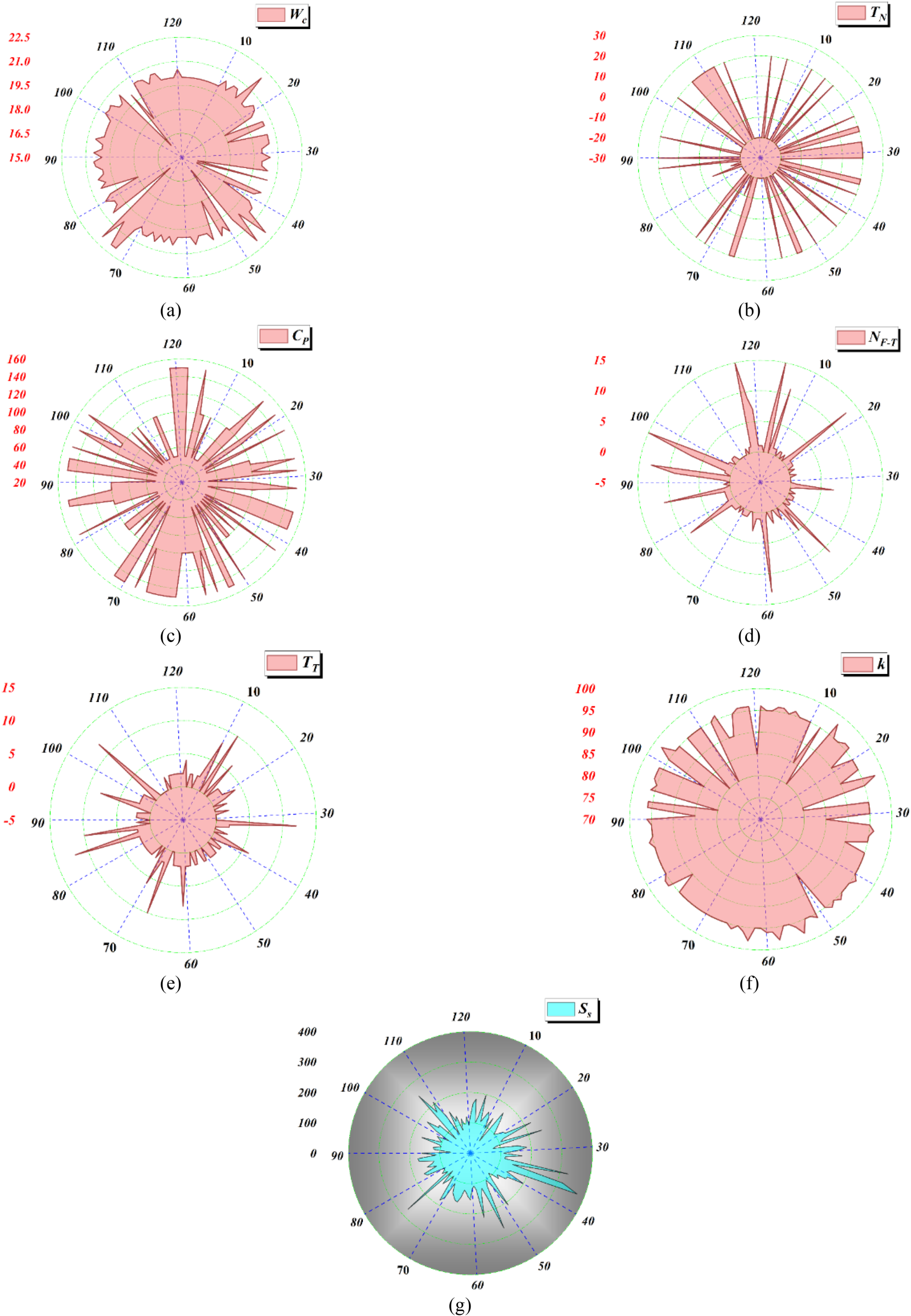
Circular Distribution of the Database.

The image displays a Pearson correlation coefficient ( $r$ ) graph. r is a statistical measure that quantifies the strength and direction of the linear link between two uninterrupted variables. It varies from −1 to 1, where −1 showcases a complete negative connection, 0 showcases no correlation, and 1 showcases a complete positive connection.

$r$ is gauged by dividing the covariance of the two variables by the product of their standard deviations. It is calculated using the following expression:

\begin{aligned} r = (Σ [(x - \bar{x}) (y - \bar{y})]) / (\sqrt [Σ (x - \bar{x})^{2}] x \sqrt [Σ (y - \bar{y})^{2}]) \end{aligned}

(1)

where:

$r$ : Pearson correlation coefficient $x$ : the value of variable $X$

$y$ : value of variable $Y$

$\bar{x}$ : mean of variable $X$ $\bar{y}$ : mean of variable $Y$

A positive value of $r$ showcases that there is a positive correlation between the two variables, meaning that as the value of one variable rises, the value of the other variable also rises. A negative value of r showcases that there is a negative correlation between the two variables, meaning that as the value of one variable rises, the value of the other variable diminishes.

The strength of the connection is identified by the magnitude of r. A value close to 1 or −1 showcases a robust connection, while a value close to $0$ showcases a poor or no correlation. r showcases the direction of the connection, with a positive sign showcasing a positive connection and a negative sign showcasing a negative correlation. r is typically utilized in investigation to identify whether there is a link between two variables and to what extent they are linked. It is noteworthy that correlation does not imply causation, and other factors may be responsible for the observed link between the variables. The overall analysis of Figure 2 reveals that there is generally no substantial connection between the diverse metrics. This implies that there will be less difficulty in developing the model, as the convergence of the model will occur more easily. The only relatively high correlations observed are between parameters $T_{n}$ and $N_{F - T}$ , $T_{n}$ and $T_{T}$ , and $N_{F - T}$ and $T_{T}$ , with R² of −0.842, −0.86, and 0.709, accordingly.

Figure 2.

The Spearman Rank Correlation Coefficient.

2.2 Algorithms and Methods

2.2.1 Golden Jackal Optimization Algorithms ( $G J O A$ )

$G J O$ replicates the congestion intellect observed in biological systems, specifically the predation patterns of golden jackals. The predation process consists of three stages: (1) victim recognition, (2) siege and incitement, and (3) assail to the victim (Chopra & Ansari, 2022). The next part explains the math used in the $G J O$ method.

The model of quest

In the initial stage, the situation of the victim is represented by an accidental matrix (Chopra & Ansari, 2022):

\begin{aligned} [\begin{array}{ccccc} Y_{1, 1} & Y_{1, j} & \dots & \dots & Y_{1, n} \\ Y_{2, 1} & Y_{2, j} & \dots & \dots & Y_{2, n} \\ \dots & \dots & \dots & \dots & \dots \\ \dots & \dots & \dots & \dots & \dots \\ Y_{N, 1} & Y_{N, j} & \dots & \dots & Y_{N, n} \end{array}] \end{aligned}

(2)

Here, N depicts the count of victim crowd and n displays the dimensions.

Discovery Stage

Catching the victim is not an easy task owing to the inherent capability of jackals to track their targets (Akbarzadeh et al., 2022). As a result, the jackals will patiently wait for another opportunity to catch their victim. The predation conduct can be described by the below equations, where the absolute value of E is more than 1 (Chopra & Ansari, 2022):

\begin{aligned} Y_{1} (t) & = Y_{M} (t) - E . | Y_{M} (t) - r l . v i c t i m (t) | \end{aligned}

(3)

\begin{aligned} Y_{2} (t) & = Y_{F M} (t) - E . | Y_{F M} (t) - r l . v i c t i m (t) | \end{aligned}

(4)

In the algorithm's current repetition, the male and female jackals are represented by $Y_{M} (t)$ and $Y_{F M} (t)$ respectively, while $v i c t i m (t)$ depicts the vector for the predation situation. The updated situations of the jackals are determined by $Y_{1} (t)$ and $Y_{2} (t)$ .

The calculation for the volatile energy of the victim $(E)$ will be performed using the formula (Chopra & Ansari, 2022)

\begin{aligned} E & = E_{1} . E_{0}, E_{0} = 2. r - 1 \end{aligned}

(5)

\begin{aligned} E_{1} & = c_{1} . (1 - \frac{t}{T}) \end{aligned}

(6)

The variables used in the calculation are as follows: $E_{0}$ is an accidentally generated number among −1 and 1, T depicts the highest number of repetitions, $c_{1}$ is fixed with a value of 1.5, and $E_{1}$ displays the decline in the victim's energy. These variables are utilized in the formula (Chopra & Ansari, 2022).

In Equations (3) and (4), the expression $| Y_{M} (t) - r l . v i c t i m (t) |$ displays the space between the jackal and the victim. The variable “ $r l$ ” displays the vector of accidental numbers identified using the Le'vy flight function $(L F)$ (Chopra & Ansari, 2022).

\begin{aligned} r l & = \frac{5. L F (y)}{100} \end{aligned}

(7)

\begin{aligned} L F (y) & = \frac{μ . σ}{100. | ϑ^{\frac{1}{β}} |}, σ = {\frac{Γ (1 + β) . \sin (\frac{π β}{2})}{Γ (\frac{1 + β}{2}) . β . (2^{β - 1})}}^{\frac{1}{β}} \end{aligned}

(8)

In the calculation, the variable “ $ϑ$ ” displays accidentally generated values within the interval (0, 1), while “ $β$ ” is a specified numerical value of 1.5 (Chopra & Ansari, 2022).

\begin{aligned} Y (t + 1) = \frac{Y_{1} (t) + Y_{2} (t)}{2} \end{aligned}

(9)

The variable $Y (t \; + \; 1)$ shows the updated situation of the victim toward the jackals.

The process of exploiting the victim, which includes besieging and devouring it, is referred to as utilization.

The harassment by golden jackals leads to a decline in the volatile energy of the victim. The conduct of jackals during the process of siege and devouring their victim can be modeled in this context, where the absolute value of E is less than or equal to 1 (Chopra & Ansari, 2022).

\begin{aligned} Y_{1} (t) & = Y_{M} (t) - E . | r l . Y_{M} (t) - v i c t i m (t) | \end{aligned}

(10)

\begin{aligned} Y_{2} (t) & = Y_{F M} (t) - E . | r l . Y_{F M} (t) - v i c t i m (t) | \end{aligned}

(11)

The conveyance from the discovery phase to the utilization phase and convergence occurs.

The $G J O$ algorithm utilizes the conveyance of the discovery stage to the utilization of the volatile energy of the victim. As the victim volatiles, its energy experiences a significant decline (Esmaeili & Mtibaa, 2024a). Taking this into consideration, the volatile energy of the victim is modeled. In each repetition, the primitive energy $E_{0}$ is accidentally deviated between −1 and 1 without any discrimination. When the energy declines from 0 to −1, it showcases that the victim is in hazard. Conversely, if it increases from 0 to 1, it signifies that the victim's ability has been increased. The volatile energy of the victim declines as the count of iterations enhances. Whenever the absolute value of E is more than 1, each pair of jackals searches various areas to detect the victim. The utilization stage is formed when the absolute value of E is less than 1, through assaulting the victim. The quest in the $G J O$ begins by considering a crowd of chosen solutions. The algorithm keeps going and uses two jackals to figure out where the victim is. The situation of each candidate's response is continuously updated in relation to the pair of jackals. By decreasing the value of $E_{1}$ from 1.5 to 0, both the discovery and utilization phases are facilitated. When the condition $E \; > \; 1$ is met, the pair of jackals stray from the victim. On the other hand, when the condition $E \; < \; 1$ is satisfied, the pair of jackals successfully gets the victim. Eventually, when the convergence conditions are met, the $G J O$ algorithm stops. Algorithm 1 shows the $G J O$ pseudo-code (Figures 3 and 4).

Figure 3.

(A) Pair of Golden Jackal, (B) Golden Jackal Searching for Prey, (C) Stalking and Enclosing of Prey, (D and E) Pouncing on Prey.

Figure 4.

Attacking Versus Looking for Prey (Chopra & Ansari, 2022).

Algorithm 1.

The pseudo-code of $G J O$ (Chopra & Ansari, 2022).

2.2.2

R F

Analysis

Accidental Forest $(R F)$ is an ensemble analysis technique drawing on DT (Breiman, 1996). $R F$ requires minimal input parameters and and little hyper-parameter adjustment (Esmaeili & Mtibaa 2024b). The $D T$ has a tree structure that illustrates the ranking of instances. The $D T$ has nodes and edges that point in a specific direction. According to (Hashemizadeh et al., 2021), the $D T$ has two kinds of nodes: inner nodes, which represent properties and leaf nodes, which represent classes. The nature of a $D T$ is to address a collection of conditional statements. In a $D T$ , each inner node illustrates a condition linked with the tree model logic, while each leaf node provides the conclusion according to the tree model logic. Once a sample enters the $D T$ , it follows only one path through the tree.

In $R F$ , a collection of multiples $D T s$ is used (Rezaei et al., 2023). The $R F$ algorithm first randomly extracts training samples from the training collection with replacement. The sub models in $R F$ are trained using the novel training collection obtained through random sampling. The ranking approach involves a method, where the final category is identified by the sub-model with the highest count of votes (Breiman, 1996). Approximately 63.2% of the samples in the primary training collection are present in the sampled collection. One benefit is that each learner utilizes only 63.2% of the samples, allowing the remaining 36.8% to be used for conducting an out-of-bag approximation (Breiman, 1996). The formula for the out-of-bag approximation is represented by equation (12).

\begin{aligned} H^{o o b} (x) = a r g m a x_{y \in γ} \\ \sum_{t = 1}^{T} I I (h_{t} (x) = y) \cdot I I (x \neq D_{t}) \end{aligned}

(12)

In the equation, $D_{t} \;$ displays the true sample set employed by $h_{t}$ , and $H^{o o b} (x)$ depicts the out-of-bag fault on sample collection x. The out-of-bag approximation formula for the generalization fault of bagging is given by equation (13).

\begin{aligned} \in^{o o b} = \frac{1}{| D |} \sum_{(x, y) \in D} I I (H^{o o b} (x) \neq y) \end{aligned}

(13)

Each tree's training collection is unique and contains duplicated training specimens. Another property of $R F$ is that, unlike $D T$ , each split procedure of the tree in $R F$ does not utilize all the properties for choice. In $R F$ , the property choice procedure differs from $D T$ . Instead of considering all properties, $R F$ accidentally selects a subset of properties from the available properties. From this accidentally chosen subset, the optimal property is chosen for each split. This accidental property choice helps to introduce diversity among the trees in the forest and reduces the correlation between them. Hence, $R F s$ are less prone to overfitting and exhibit strong resistance to noise. Furthermore, the key control parameters of $R F$ encompass the correlation between individual trees within the forest, the ranking capability of each tree, and the count of properties chosen.

Boosting the pivotal parameters the $R F$ is crucial for enhancing the productivity of the classification and attaining superior outcomes in this research. The exploration mainly concentrated on three basic factors: $n_e s t i m a t o r s$ , $m a x_d e p t h$ , and $m a x_f e a t u r e s$ . The quantity of DT is displayed by the term $n_e s t i m a t o r s$ . $m a x_d e p t h$ showcases the maximum depth of DTs, whereas $m a x_f e a t u r e s$ showcases the maximum count of features used in DTs. $n_e s t i m a t o r s$ was appointed a value ranging from 1 to 100, with increments of 5 between each value. The $m a x_d e p t h$ parameter was adjusted to a value within the range of 10 to 100, with an increment of 5. The parameter $m a x \; f e a t u r e s$ was appointed a value ranging from 1 to 100, with an increment of one. Enhancement techniques may be used to determine the optimal values for the vital elements mentioned. The goal was fulfilled by deploying $G J O$ in this exploration.

2.2.3

L S S V R

River flow forecast using the Hybrid $L S S V R$ -Gravitation Search Algorithm $(H L G S A)$ technique. The least square support vector regression (LSSVR) method, presented by Suykens and Vandewalle (Suykens & Vandewalle, 1999), is a adjusted version of $S V R$ . It offers benefits over $S V R$ by simplifying the optimization procedure through the use of linear equations instead of quadratic equations (Xiaohui & Xiaoping, 2010). Figure 1 illustrates the step-by-step procedure of the $L S S V R$ algorithm. The nonlinear $L S S V R$ function is defined by employing time series inputs $x_{i}$ (delayed river flows) and output $y_{i}$ (forecasted river flow).

\begin{aligned} y (x) = ⟨ ω^{T}, φ (x) ⟩ + b \end{aligned}

(14)

In the given context, the weight vector $ω$ and bias term b are accompanied by a nonlinear function $φ (x)$ that utilizes regression and the dot product illustrated by $⟨ \cdot, \cdot ⟩$ (Arabloo et al., 2015). The minimization of the cost function $(C)$ in $L S S V R$ can be achieved by:

Min,

\begin{aligned} C = \frac{1}{2} ω^{t} ω + \frac{γ}{2} \sum_{i = 1}^{n} e_{i}^{2} \end{aligned}

(15)

Subject to,

\begin{aligned} y_{i} = ⟨ ω, φ (x) ⟩ + b + e_{i}, i = 1, 2, \dots, n \end{aligned}

(16)

In this context,

γ

illustrates the ordered fixed and

e_{i}

displays the training fault for

x_{i}

. To find the solutions for

ω

and e in equation (15), the Lagrange function is employed. The calculation of the Lagrange function can be expressed as (Suykens et al., 2002).

\begin{aligned} L_{L S S V R} = C - \\ \sum_{i = 1}^{N} α_{i} {⟨ ω, φ (x) ⟩ + b + e_{i} - y_{i}} \end{aligned}

(17)

In this case, $α_{i} \in R$ displays the Lagrange multipliers. The solution to the above equation can be obtained by taking the partial derivative of the Lagrange function and including the kernel function $(K F)$ to realize $M e r c e r^{'} s$ condition. For solving regression issues, various kinds of kernel functions $(K F)$ can be utilized, including polynomial, radial basis, Gaussian, sigmoid, Mexican hat, Meyer, and Morlet. The kind of kernel function $(K F)$ utilized is crucial in manufacturing a highly precise $L S S V R$ model (Yuan et al., 2015). Due to its effectiveness in solving nonlinear regression issues (Shi et al., 2012), the radial basis kernel function $(R B K F)$ was utilized in this study. Part 7 presents a comparison of the function of $R B K F$ with other kinds of kernel functions. $\; (R B K F)$ could be written as follows:

\begin{aligned} K (x_{i}, x_{j}) = e x p (- \frac{{| | x_{i} - x_{j} | |}^{2}}{σ^{2}}) \end{aligned}

(18)

Once the $R B K F$ has been chosen for the $L S S V R$ method, it is obligate to determine appropriate values for the fine agent parameter $(γ)$ and the $R B K F$ parameter ( $σ^{2}$ ). There is no definitive method for obtaining the optimal values of parameters. To address these challenges, the study adopted the $(G S A)$ to compute the appropriate parameter values.

The previous clarification demonstrates how the $L S S V R$ framework's regression findings are directly impacted by the penalty factor ( $c$ ) and kernel function width ( $g$ ). Underfitting is more probable when c is smaller. Conversely, as c increases, the error tolerance decreases while the likelihood of overfitting increases (Wu & Ye, 2016). The parameter g is also used in $L S S V R$ to modify the mapping procedure from low-dimensional tests to high-dimensional samples. The mapping dimension and the value of g are positively correlated. Accordingly, a larger value of g results in an increase in the mapping dimension and an enhancement of the education impact. The propensity for over-fitting increases with g, which hinders generalization (Ghaedi et al., 2016). As a result, anytime g is implemented, it is crucial to choose the correct quantity. Setting g to a very big value may result in input patterns that are too identical, hence increasing the difficulty for the function to precisely fit the data. When the value of g is very tiny, the resulting design may seem highly unusual, perhaps resulting in overfitting (Goyal et al., 2014). This research utilizes the $G J O$ method to identify the optimal values for the parameters c and g, ensuring that the framework precisely displays the desired outcomes.

The optimization of hyperparameters with the $G J O$ method was essential in regulating model complexity, hence averting excessive specialization to the training data. Moreover, performance was assessed via both training and testing phases, with the models continually attaining excellent accuracy at each step. This methodology, together with the minimal objective function values, showcases that the models are well-calibrated, guaranteeing reliable predictions without overfitting (Asteris et al., 2021b; Benzaamia et al., 2024).

2.3 Metrics

The creation of effectiveness comparison measures was motivated by the need for a standardized and quantitative tactic to appraise and compare the general efficacy of diverse approaches. As part of their inquiry, the academics gauged the subsequent measurements and included their findings in the examination:

$R^{2}$

\begin{aligned} R^{2} = {(\frac{\sum_{g = 1}^{G} (n_{g} - \bar{n}) (z_{g} - \bar{y})}{\sqrt{[\sum_{g = 1}^{G} {(n_{g} - n)}^{2}] [\sum_{g = 1}^{G} {(y_{g} - \bar{y})}^{2}]}})}^{2} \end{aligned}

(19)

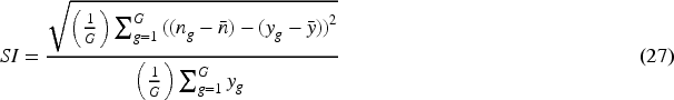
Root mean square error ( $R M S E$ )

\begin{aligned} R M S E = \sqrt{\frac{1}{G} \sum_{g = 1}^{G} {(y_{g} - n_{g})}^{2}} \end{aligned}

(20)

Normalized root-mean-square ( $N R M S E$ )

\begin{aligned} N R M S E = R M S E / \bar{y} \end{aligned}

(21)

Relative absolute error ( $R A E$ )

\begin{aligned} R A E = \frac{\sum_{g = 1}^{G} | n_{g} - y_{g} |}{\sum_{g = 1}^{G} | n_{g} - \bar{n} |} \end{aligned}

(22)

Root relative square error ( $R R S E$ )

\begin{aligned} R R S E = \sqrt{\frac{\sum_{g = 1}^{G} {(n_{g} - y_{g})}^{2}}{\sum_{g = 1}^{G} {(n_{g} - \bar{n})}^{2}}} \end{aligned}

(23)

Mean absolute error ( $M A E$ )

\begin{aligned} M A E = \frac{1}{G} \sum_{g = 1}^{G} | y_{g} - n_{g} | \end{aligned}

(24)

Performance index

\begin{aligned} P I = \frac{1}{\bar{n}} \times \frac{R M S E}{\sqrt{R^{2} + 1}} \end{aligned}

(25)

Variance account factor ( $V A F$ )

\begin{aligned} V A F = (1 - \frac{v a r (n_{g} - y_{g})}{v a r (n_{g})}) * 100 \end{aligned}

(26)

Scatter index

\begin{aligned} S I = \frac{\sqrt{(\frac{1}{G}) \sum_{g = 1}^{G} {((n_{g} - \bar{n}) - (y_{g} - \bar{y}))}^{2}}}{(\frac{1}{G}) \sum_{g = 1}^{G} y_{g}} \end{aligned}

(27)

a10 index (Asteris et al., 2024; Asteris et al., 2021a)

\begin{aligned} a 10 = \frac{g_{10}}{G} \end{aligned}

(28)

$O B J$ (A comprehensive index)

\begin{aligned} O B J = {(\frac{g}{G} \times \frac{R M S E + M A E}{R^{2} + 1})}^{T r a i n} + {(\frac{g}{G} \times \frac{R M S E + M A E}{R^{2} + 1})}^{T e s t} \end{aligned}

(29)

where:

$n_{g}$ : the measured $S_{s}$

$\bar{n}$ : the mean of the measured $S_{s}$

$y_{g}$ : the forecasted $S_{s}$

$\bar{y}$ : the mean of the forecasted $S_{s}$

$G$ : the count of rows of the database

$g_{t r a i n}$ : the count of databases in the training subset

$g_{t e s t}$ : the count of databases in the testing subset

3. Results and Discussion

3.1 Process of Models

The creation of optimization-based models comprised the implementation of the following stages: (a) Configuring the first $L S S V R$ and $R F$ simulations was the first step, (b) The created collection was then arbitrarily separated into training and testing subgroups, (c) the $G J O$ method was used in conjunction with the initialized $L S S V R$ and $R F$ models (also known as $L S G J$ and $R F G J$ ), (d) after attaining the desired goal function, the ideal values for each model's hyperparameters were explored (see Table 2).

Table 2.
The Initialization Process and Tunned Values.

Algorithms Main or tunned parameters Initial or tunned values

$G J O$ Max number of iterations 100

Number of runs 10

Number of populations 15

$C_{1}$ [1–2]

$L S S V R \to L S G J$ $c$ [1–100] 23.7

$g$ [0.5–5] 2.028

$R F \to R F G J$ $n_e s t i m a t o r s$ [1–100] 73

$M a x_d e p t h$ [10–100] 29

$M a x_f e a t u r e s$ [1–100] 35

Algorithms	Main or tunned parameters	Initial or tunned values
$G J O$	Max number of iterations	100
Number of runs	10
Number of populations	15
$C_{1}$	[1–2]
$L S S V R \to L S G J$	$c$ [1–100]	23.7
$g$ [0.5–5]	2.028
$R F \to R F G J$	$n_e s t i m a t o r s$ [1–100]	73
$M a x_d e p t h$ [10–100]	29
$M a x_f e a t u r e s$ [1–100]	35

3.2 Comparison of Frameworks

This paper presents the results of integrating the $G J O$ process with $L S S V R$ and $R F$ approaches. Utilizing the methods described above, $S_{s}$ of seasonally frozen soils was identified. Figure 5 displays the expected and actual values of $S_{s}$ for each of the two distinct combined methods that were created— $L S G J$ and $R F G J$ —during the learning and testing periods. In addition, the following figure displays the range of error frequencies. The estimation effectiveness of the methods for $S_{s}$ was evaluated using a variety of measurements, including $R^{2}$ , $R M S E$ , $N R M S E$ , $R A E$ , $R R S E, M A E$ , $P I$ , $V A F$ , $S I$ , and an all-inclusive index called $O B J$ . A thorough description of the outcomes of the metrics included in the models is depicted in Table 3. Additionally, the present exploration compares and contrasts the results with those of a before-published publication that employed $A N N$ and $P C A - A N N$ in an effort to determine the efficacy of the approaches (Sun et al., 2023).

Figure 5.

The Models’ Outcomes, Left: Correlation, Right: Error (%) (a: Train Subset, b: Test Subset).

Table 3.

The Results of Regression Models.

			Regression analysis		(Sun et al., 2023)
Index		Subset	$LSGJ$	$RFGJ$	$ANN$	$PCA - ANN$
$R^{2}$	Good is high	Train	0.9905	0.9865	0.97	0.97
$R^{2}$	Good is high	Test	0.9952	0.9889	0.96	0.97
$RMSE$ ( $k P a$ )	Good is low	Train	5.2209	6.3178	8.1	8.6
$RMSE$ ( $k P a$ )	Good is low	Test	3.0196	4.4799	11.9	10.7
$NRMSE$	Good is low	Train	0.0361	0.0437
$NRMSE$	Good is low	Test	0.0239	0.0354
$RAE$	Good is low	Train	0.0695	0.0976
$RAE$	Good is low	Test	0.0544	0.0859
$RRSE$	Good is low	Train	0.0978	0.1183
$RRSE$	Good is low	Test	0.0734	0.109
$MAE$	Good is low	Train	2.5539	3.5891	5.7	6.1
$MAE$	Good is low	Test	1.6916	2.6701	8.1	7.7
$PI$	Good is low	Train	0.018	0.0219
$PI$	Good is low	Test	0.0121	0.0179
$VAF$	Good is high	Train	99.0472	98.6061
$VAF$	Good is high	Test	99.5102	98.8932
$SI$	Good is low	Train	0.036	0.0436
$SI$	Good is low	Test	0.0241	0.0358
a10 index	Good is high	Train	99.002	98.78
a10 index	Good is high	Test	99.113	98.589
$OBJ$	Good is low	Overall	3.5198	4.6391

The results obtained reveal that the $L S G J$ and $R F G J$ methods possess a significant ability to accurately anticipate the $S_{s}$ of seasonally frozen soils. During the training and testing stages, the $R^{2}$ and $V A F$ values for the $L S G J$ network were found to be, respectively, 0.9905 and 0.9952 and 99.047% and 99.5102%. With $R^{2}$ values of 0.9865 and 0.9889 and $V A F$ of 98.6061% and 98.893%, respectively, these values were higher than the $R F G J$ . During the estimating period, all of the models demonstrated high performance and accuracy levels. Other error-based metrics, such as $R M S E$ , $N R M S E$ , $R A E$ , $R R S E$ , $M A E$ , $P I$ , and $S I$ , may be helpful in determining the approach's accuracy. The values of these indicators demonstrate that $L S G J$ operates more effectively than $R F G J$ , if only somewhat, by attaining smaller values than the other. Last but not least, it was observed that $L S G J$ gets the fewest value on the $O B J$ scale, the lower the best, at 3.5198, which is over 30% less than $R F G J$ at 4.6391.

Additionally, a comparison between the outperforming models ( $L S G J$ ) outcomes ( $R^{2}$ , $R M S E$ , and $M A E$ ) and the conclusions from the literature on the $A N N$ and $P C A - A N N$ systems (Sun et al., 2023) are shown in Table 3. It is clear from the comparison that although the performance of the literature's models was acceptable, the model developed in this article presented better workability, by achieving higher $R^{2}$ , and lower values of the $R M S E$ and $M A E$ in training and testing. For example, $R^{2}$ at 0.97 for $A N N$ and $P C A - A N N$ (Sun et al., 2023) lower than 0.9905 for $L S G J$ in the training phase, and 0.96 compared to 0.9952 in the testing stages. Other metrics (i.e., $M A E$ and $R M S E$ ) depicted extremely improvement especially in the testing database.

On the right side of Figure 5, you can see the error percent dispersion of the estimates made by the two $L S G J$ and $R F G J$ approaches during training and testing. A smaller error % range with a lowest and maximum bound showcases higher accuracy. A larger degree of error variability in the data suggests that $R F G J$ is less effective in two phases. When using the $G J O$ method to improve the $L S S V R$ model, a substantial incidence of errors is seen. This is especially noticeable when the error % is close to zero and falls below predetermined criteria.

3.3 Limitations

The models may be tailored to the specific characteristics of the database used, raising concerns about their generalizability to different geographical locations, soil types, or environmental conditions. It acquired a more diverse database that displays a broader range of geographical locations, soil types, and environmental conditions. This can enhance the generalizability of the models. Consider collecting longitudinal data to capture changes in soil properties over time. If the properties of the seasonally frozen soils change over time or under different conditions, the assumption of stationarity may not hold, impacting the model's accuracy over the long term. Machine learning models, like $R F$ and $S V R$ , are often considered “black-box” models, making it challenging to interpret the links amid input variables and the model's predictions. The models in real-world field conditions can be validated to assess their practical applicability and accuracy in predicting the static strength of seasonally frozen soils in situ.

4. Conclusions

Two machine learning-based methods for assessing $S_{s}$ of seasonally frozen soils were developed and verified in the current research. Two strong and dependable methods were taken into consideration: $R F$ and $L S S V R$ . Each of these algorithms has important hyperparameters that have a significant impact on the accuracy of the model. Optimization methods may be used to identify these hyperparameters optimally; in this work, the $G J O$ was used to achieve this goal (called $R F G J$ and $L S G J$ ).

The results obtained indicate that the $L S G J$ and $R F G J$ methods possess a significant ability to accurately anticipate the $S_{s}$ of seasonally frozen soils. During the training and testing stages, the $R^{2}$ and $V A F$ values for the $L S G J$ network were found to be, respectively, 0.9905 and 0.9952 and 99.047% and 99.5102%. With $R^{2}$ values of 0.9865 and 0.9889 and $V A F$ of 98.6061% and 98.893%, respectively, these values were higher than the $R F G J$ . During the estimating period, all of the models demonstrated high performance and accuracy levels.

It was observed that $L S G J$ gets the fewest value on the $O B J$ scale, at 3.5198, which is over 30% less than $R F G J$ at 4.6391.

Although the performance of the literature's models was acceptable, the framework created in this article presented better workability, by attaining higher $R^{2}$ , and lower values of the $R M S E$ and $M A E$ in training and testing. For example, $R^{2}$ at 0.97 for $A N N$ and $P C A - A N N$ (Karbassi et al., 2014) lower than 0.9905 for $L S G J$ in the training phase, and 0.96 compared to 0.9952 in the testing stages. Other metrics (i.e., $M A E$ , and $R M S E$ ) depicted extremely improvement especially in the testing database.

Because the models use certain database properties, they may not apply to varied geographical locations, soil types, and environmental circumstances. Adding variability to the database improves generalizability. Since seasonally frozen soils may not be stationary, longitudinal data collection is essential to capture temporal changes in soil characteristics and ensure long-term accuracy. In addition, “black-box” approaches like $R F$ and $S V R$ make input–output interpretation difficult. Field validation is necessary to assess the models’ utility in forecasting seasonally frozen soil static strength.

The models may be used for infrastructure design, risk assessment, and material optimization in seasonally frozen soils. They reliably forecast freeze–thaw static strength degradation to help engineers build lasting foundations, pavements, and embankments. The models also measure structural stability, reducing failure risks and maintenance costs. These models may also help choose and optimize soil stabilizing methods and materials for better performance in different environments.

Footnotes

Funding

The authors disclosed receipt of the following financial support for the research, authorship, and/or publication of this article: The project funded by Heilongjiang Natural Science Foundation No. LH2023D021 Project name. The research focuses on investigating the freeze-thaw stability mechanism of roadbeds based on the non-thermal equilibrium theory of porous media.

Declaration of Conflicting Interests

The authors declared no potential conflicts of interest with respect to the research, authorship, and/or publication of this article.

References

Adeli Ghareh Viran

Binal

(2018). Effects of repeated freeze–thaw cycles on physico-mechanical properties of cohesive soils. Arabian Journal of Geosciences, 11, 1–13. https://doi.org/10.1007/s12517-018-3592-5

Afkhami Hoor

Esmaeili-Falak

(2024). Innovative Approaches for Mitigating Soil Liquefaction: A State-of-the-Art Review of Techniques and Bibliometric Analysis. Indian Geotechnical Journal, 120, 273. https://doi.org/10.1007/s40098-024-01120-3

Akbarzadeh

Karami

Fasihihour

Alghanim

Hamzehei

(2022). Multicast Optimization: Operational Research Theory and Applications. 2022 International Engineering Conference on Electrical, Energy, and Artificial Intelligence (EICEEAI), pp. 1–4. https://doi.org/10.1109/EICEEAI56378.2022.10050486

Alkayem

N. F.

Shen

Mayya

Asteris

P. G.

Di Luzio

Strauss

Cao

(2024). Prediction of concrete and FRC properties at high temperature using machine and deep learning: A review of recent advances and future perspectives. Journal of Building Engineering, 83, 108369. https://doi.org/10.1016/j.jobe.2023.108369

Arabloo

Ziaee

Lee

Bahadori

(2015). Prediction of the properties of brines using least squares support vector machine (LS-SVM) computational strategy. Journal of the Taiwan Institute of Chemical Engineers, 50, 123–130. https://doi.org/10.1016/j.jtice.2014.12.005

Asteris

P. G.

Karoglou

Skentou

A. D.

Vasconcelos

Bakolas

Zhou

Armaghani

D. J.

(2024). Predicting uniaxial compressive strength of rocks using ANN models: Incorporating porosity, compressional wave velocity, and schmidt hammer data. Ultrasonics, 141, 107347. https://doi.org/10.1016/j.ultras.2024.107347

Asteris

P. G.

Koopialipoor

Armaghani

D. J.

Kotsonis

E. A.

Lourenço

P. B.

(2021a). Prediction of cement-based mortars compressive strength using machine learning techniques. Neural Computing & Applications, 33(19), 13089–13121. https://doi.org/10.1007/s00521-021-06004-8

Asteris

P. G.

Skentou

A. D.

Bardhan

Samui

Pilakoutas

(2021b). Predicting concrete compressive strength using hybrid ensembling of surrogate machine learning models. Cement and Concrete Research, 145, 106449. https://doi.org/10.1016/j.cemconres.2021.106449

Aydin

Sivrikaya

Uysal

(2020). Effects of curing time and freeze–thaw cycle on strength of soils with high plasticity stabilized by waste marble powder. Journal of Material Cycles and Waste Management, 22(5), 1459–1474. https://doi.org/10.1007/s10163-020-01035-0

10.

Benemaran

R. S.

Esmaeili-Falak

(2023). Predicting the Young’s modulus of frozen sand using machine learning approaches: State-of-the-art review. Geomechanics and Engineering, 34(5), 507–527. https://doi.org/10.12989/gae.2023.34.5.507

11.

Benzaamia

Ghrici

Rebouh

Zygouris

Asteris

P. G.

(2024). Predicting the shear strength of rectangular RC beams strengthened with externally-bonded FRP composites using constrained monotonic neural networks. Engineering Structures, 313, 118192. https://doi.org/10.1016/j.engstruct.2024.118192

12.

Breiman

(1996). Bagging predictors. Machine Learning, 24, 123–140. https://doi.org/10.1007/BF00058655

13.

Chopra

Ansari

M. M.

(2022). Golden jackal optimization: A novel nature-inspired optimizer for engineering applications. Expert Systems With Applications, 198, 116924. https://doi.org/10.1016/j.eswa.2022.116924

14.

Das

S. K.

Samui

Sabat

A. K.

(2011). Application of artificial intelligence to maximum dry density and unconfined compressive strength of cement stabilized soil. Geotechnical and Geological Engineering, 29, 329–342. https://doi.org/10.1007/s10706-010-9379-4

15.

Das

S. K.

Samui

Sabat

A. K.

Sitharam

T. G.

(2010). Prediction of swelling pressure of soil using artificial intelligence techniques. Environmental Earth Sciences, 61, 393–403. https://doi.org/10.1007/s12665-009-0352-6

16.

Dawei

Bing

Bingbing

Xibo

Razzaghzadeh

(2023). Predicting the CPT-based pile set-up parameters using HHO-RF and PSO-RF hybrid models. Structural Engineering and Mechanics: An International Journal, 86(5), 673–686.

17.

Ebrahim

Mahzad

E.-F.

(2024). Soil–structure interaction for buried conduits influenced by the coupled effect of the protective layer and trench installation. Journal of Pipeline Systems Engineering and Practice, 15(2), 04024012. https://doi.org/10.1061/JPSEA2.PSENG-1547

18.

Esmaeili

Mtibaa

(2024a). SAMBA: Scalable Approximate Forwarding For NDN Implicit FIB Aggregation. 2024 IEEE 13th International Conference on Cloud Networking (CloudNet), IEEE, pp. 1–9.

19.

Esmaeili

Mtibaa

(2024b) SERENE: A Collusion Resilient Replication-based Verification Framework, ArXiv Preprint ArXiv:2404.11410.

20.

Esmaeili-Falak

Benemaran

R. S.

(2024). Ensemble extreme gradient boosting based models to predict the bearing capacity of micropile group. Applied Ocean Research, 151, 104149. https://doi.org/10.1016/j.apor.2024.104149

21.

Esmaeili-Falak

Katebi

Javadi

(2018). Experimental study of the mechanical behavior of frozen soils-A case study of Tabriz subway. Periodica Polytechnica Civil Engineering, 62(1), 117–125. https://doi.org/10.3311/PPci.10960

22.

Esmaeili-Falak

Katebi

Javadi

Rahimi

(2017). Experimental investigation of stress and strain characteristics of frozen sandy soils-A case study of Tabriz subway. Modares Civil Engineering Journal, 17(5), 13–23. http://mcej.modares.ac.ir/article-16-7658-en.html

23.

Esmaeili-Falak

Katebi

Vadiati

Adamowski

(2019). Predicting triaxial compressive strength and Young’s modulus of frozen sand using artificial intelligence methods. Journal of Cold Regions Engineering, 33(3), 04019007. https://doi.org/10.1061/(ASCE)CR.1943-5495.0000188

24.

Fan

Yang

Z. J.

Yang

(2020). A model for evaluating settlement of clay subjected to freeze-thaw under overburden pressure. Cold Regions Science and Technology, 173, 102996. https://doi.org/10.1016/j.coldregions.2020.102996

25.

Garg

Wani

Zhu

Kushvaha

(2022). Exploring efficiency of biochar in enhancing water retention in soils with varying grain size distributions using ANN technique. Acta Geotechnica, 17(4), 1315–1326. https://doi.org/10.1007/s11440-021-01411-6

26.

Ghaedi

reza Rahimi

Ghaedi

A. M.

Tyagi

Agarwal

Gupta

V. K.

(2016). Application of least squares support vector regression and linear multiple regression for modeling removal of methyl orange onto tin oxide nanoparticles loaded on activated carbon and activated carbon prepared from Pistacia atlantica wood. Journal of Colloid and Interface Science, 461, 425–434. https://doi.org/10.1016/j.jcis.2015.09.024

27.

Goyal

M. K.

Bharti

Quilty

Adamowski

Pandey

(2014). Modeling of daily pan evaporation in sub tropical climates using ANN, LS-SVR, fuzzy logic, and ANFIS. Expert Systems With Applications, 41(11), 5267–5276. https://doi.org/10.1016/j.eswa.2014.02.047

28.

Habibagahi

Bamdad

(2003). A neural network framework for mechanical behavior of unsaturated soils. Canadian Geotechnical Journal, 40(3), 684–693. https://doi.org/10.1139/t03-004

29.

Han

Wang

Zhang

Cheng

Kong

(2018). Effect of freeze-thaw cycles on shear strength of saline soil. Cold Regions Science and Technology, 154, 42–53. https://doi.org/10.1016/j.coldregions.2018.06.002

30.

Hao

Cui

Zheng

Bao

(2022). Dynamic behavior of thawed saturated saline silt subjected to freeze-thaw cycles. Cold Regions Science and Technology, 194, 103464. https://doi.org/10.1016/j.coldregions.2021.103464

31.

Hashemizadeh

Maaref

Shateri

Larestani

Hemmati-Sarapardeh

(2021). Experimental measurement and modeling of water-based drilling mud density using adaptive boosting decision tree, support vector machine, and K-nearest neighbors: A case study from the South Pars gas field. Journal of Petroleum Science and Engineering, 207, 109132. https://doi.org/10.1016/j.petrol.2021.109132

32.

Hastie

Tibshirani

Friedman

J. H.

Friedman

J. H.

(2009). The elements of statistical learning: data mining, inference, and prediction. Springer.

33.

Hou

C.-Y.

Cui

Z.-D.

Yuan

(2020). Accumulated deformation and microstructure of deep silty clay subjected to two freezing-thawing cycles under cyclic loading. Arabian Journal of Geosciences, 13, 1–13. https://doi.org/10.1007/s12517-019-5007-7

34.

Javadi

A. A.

Rezania

(2009). Applications of artificial intelligence and data mining techniques in soil modeling. Geomechanics and Engineering, 1(1), 53–74. https://doi.org/10.12989/gae.2009.1.1.053

35.

Karbassi

Mohebi

Rezaee

Lestuzzi

(2014). Damage prediction for regular reinforced concrete buildings using the decision tree algorithm. Computers & Structures, 130, 46–56. https://doi.org/10.1016/j.compstruc.2013.10.006

36.

Katariya

N. K.

Choudhary

B. S.

Esmaeili-Falak

Raina

A. K.

(2025). Analysis of floral biodiversity, survival, and growth rate in dump slope rehabilitation of an iron ore mine with jute geotextile. International Journal of Phytoremediation, 1–17. https://doi.org/10.1080/15226514.2025.2501426

37.

Kohestani

V. R.

Hassanlourad

(2016). Modeling the mechanical behavior of carbonate sands using artificial neural networks and support vector machines. International Journal of Geomechanics, 16(1), 04015038. https://doi.org/10.1061/(ASCE)GM.1943-5622.0000509

38.

Kotov

P. I.

Stanilovskaya

J. Y. V.

(2022). Predicting changes in the mechanical properties of frozen saline soils. European Journal of Environmental and Civil Engineering, 26(12), 5716–5728. https://doi.org/10.1080/19648189.2021.1916604

39.

Kou

Quan

Guo

Hassankhani

(2024). Light and normal weight concretes shear strength estimation using tree-based tunned frameworks. Construction and Building Materials, 452, 138955. https://doi.org/10.1016/j.conbuildmat.2024.138955

40.

Zhu

Zhang

Lin

(2004). Effects of temperature, strain rate and dry density on compressive strength of saturated frozen clay. Cold Regions Science and Technology, 39(1), 39–45. https://doi.org/10.1016/j.coldregions.2004.01.001

41.

Liang

Bayrami

(2023). Estimation of frost durability of recycled aggregate concrete by hybridized random forests algorithms. Steel and Composite Structures, 49(1), 91–107. https://doi.org/10.12989/scs.2023.49.1.091

42.

Lin

Zheng

Han

(2022). Comparative performance of eight ensemble learning approaches for the development of models of slope stability prediction. Acta Geotechnica, 17(4), 1477–1502. https://doi.org/10.1007/s11440-021-01440-1

43.

Liu

Chang

(2016). Influence of freeze-thaw cycles on mechanical properties of a silty sand. Engineering Geology, 210, 23–32. https://doi.org/10.1016/j.enggeo.2016.05.019

44.

(2024). Prediction of gasification process via random forest regression model optimized with meta-heuristic algorithms. Journal of Artificial Intelligence and System Modelling, 1(02), 45–65. https://doi.org/10.22034/jaism.2024.445930.1026

45.

Qian

(2023). Maximum dry unit weight and optimum moisture content prediction of lateritic soils using regression analysis. Advances in Engineering and Intelligence Systems, 2(01), 15–26. https://doi.org/10.22034/aeis.2023.374474.1059

46.

Rezaei

Khan

Lee

Mossé

(2023). Solar-powered parking analytics system using deep reinforcement learning. ACM Transactions on Sensor Networks, 19(4), 1–27. https://doi.org/10.1145/3584949

47.

Sarkhani Benemaran

(2023). Application of extreme gradient boosting method for evaluating the properties of episodic failure of borehole breakout. Geoenergy Science and Engineering, 226, 211837. https://doi.org/10.1016/j.geoen.2023.211837

48.

Shen

Wang

Chen

Han

Zhang

Liu

(2022). Evolution process of the microstructure of saline soil with different compaction degrees during freeze-thaw cycles. Engineering Geology, 304, 106699. https://doi.org/10.1016/j.enggeo.2022.106699

49.

Shi

D.-Y.

L.-J.

(2012). A judge model of the impact of lane closure incident on individual vehicles on freeways based on RFID technology and FOA-GRNN method. Wuhan Ligong Daxue Xuebao(Journal of Wuhan University of Technology), 34(3), 63–68.

50.

Sihag

Tiwari

N. K.

Ranjan

(2018). Prediction of cumulative infiltration of sandy soil using random forest approach. Journal of Applied Water Engineering and Research, 7(2), 118–142. https://doi.org/10.1080/23249676.2018.1497557

51.

Sun

Dong

Teng

Wang

Hassankhani

(2024). Creation of regression analysis for estimation of carbon fiber reinforced polymer-steel bond strength. Steel and Composite Structures, 51(5), 509–527. https://doi.org/10.12989/scs.2024.51.5.509

52.

Sun

Zhou

Meng

Wang

(2023). Principal component analysis–artificial neural network-based model for predicting the static strength of seasonally frozen soils. Scientific Reports, 13(1), 16085. https://doi.org/10.1038/s41598-023-43462-7

53.

Suykens

J. A. K.

De Brabanter

Lukas

Vandewalle

(2002). Weighted least squares support vector machines: Robustness and sparse approximation. Neurocomputing, 48(1-4), 85–105. https://doi.org/10.1016/S0925-2312(01)00644-0

54.

Suykens

J. A. K.

Vandewalle

(1999). Least squares support vector machine classifiers. Neural Process Lett, 9, 293–300. https://doi.org/10.1023/A:1018628609742

55.

Vahdani

Ghazavi

Roustaei

(2020). Measured and predicted durability and mechanical properties of frozen-thawed fine soils. KSCE Journal of Civil Engineering, 24(3), 740–751. https://doi.org/10.1007/s12205-020-2178-4

56.

Wei

Guodong

Qingbai

(2009). Construction on permafrost foundations: Lessons learned from the Qinghai–Tibet railroad. Cold Regions Science and Technology, 59(1), 3–11. https://doi.org/10.1016/j.coldregions.2009.07.007

57.

(2016). Fault diagnosis and prognostic of solid oxide fuel cells. Journal of Power Sources, 321, 47–56. https://doi.org/10.1016/j.jpowsour.2016.04.080

58.

Xiaohui

G. U. O.

Xiaoping

M. A.

(2010). Mine water discharge prediction based on least squares support vector machines. Mining Science and Technology (China), 20(5), 738–742. https://doi.org/10.1016/S1674-5264(09)60273-8

59.

(2020). Investigation on the behavior of frozen silty clay subjected to monotonic and cyclic triaxial loading. Acta Geotech, 15, 1289–1302. https://doi.org/10.1007/s11440-019-00826-6

60.

Wang

Yin

Zhang

(2017). Effect of temperature and strain rate on mechanical characteristics and constitutive model of frozen Helin loess. Cold Regions Science and Technology, 136, 44–51. https://doi.org/10.1016/j.coldregions.2017.01.010

61.

Yaychi

B. M.

Esmaeili-Falak

(2024). Estimating axial bearing capacity of driven piles using tuned random forest frameworks. Geotechnical and Geological Engineering, 42(8), 7813–7834. https://doi.org/10.1007/s10706-024-02952-9

62.

Fang

Zhou

(2022). The study of influence of freeze-thaw cycles on silty sand in seasonally frozen soil regions. Geofluids, 2022, 1–12. https://doi.org/10.1155/2022/6886108

63.

Yuan

Chen

Yuan

Huang

Tan

(2015). Short-term wind power prediction based on LSSVM–GSA model. Energy Conversion and Management, 101, 393–401. https://doi.org/10.1016/j.enconman.2015.05.065

64.

Zhang

Razzaghzadeh

(2024). Application of the optimal fuzzy-based system on bearing capacity of concrete pile. Steel and Composite Structures, 51(1), 25–41. https://doi.org/10.12989/scs.2024.51.1.025

65.

Zou

Han

Zhao

Fan

Vanapalli

S. K.

Wang

(2022). Effects of cyclic freezing and thawing on the shear behaviors of an expansive soil under a wide range of stress levels. Environmental Earth Sciences, 81(3), 77. https://doi.org/10.1007/s12665-022-10190-6

		Index
Subsets	Variable	Min.	Max.	St. D.	Var.	Avg.	Skew.	Kurt.
Train	Input 1: $W_{c}$	16	22	1.206	1.455	19.968	−1.875	4.775
Test	Input 1: $W_{c}$	16	20.5	0.872	0.761	19.993	−3.525	15.217
Train	Input 2: $T_{N}$	−20	20	17.83	317.914	−7.555	0.852	−1.203
Test	Input 2: $T_{N}$	−20	20	18.705	349.88	−6.333	0.6827	−1.565
Train	Input 3: $C_{P}$	50	150	40.388	1631.17	102.77	−0.1012	−1.475
Test	Input 3: $C_{P}$	50	150	40.994	1680.55	91.667	0.3158	−1.487
Train	Input 4: $N_{F - T}$	0	15	3.1584	9.9754	1.811	2.759	7.161
Test	Input 4: $N_{F - T}$	0	15	4.596	21.128	3.0667	1.555	1.491
Train	Input 5: $T_{T}$	0	12	2.6302	6.918	2.2444	2.1483	4.865
Test	Input 5: $T_{T}$	0	12	2.418	5.8489	1.8666	2.842	10.66
Train	Input 6: $k$	80	98	3.492	12.196	94.322	−2.924	8.856
Test	Input 6: $k$	80	98	5.4067	29.23	92.633	−1.416	0.803
Train	Target: $S_{S}$	50	374	53.391	2850.58	144.98	1.9446	5.112
Test	Target: $S_{S}$	65	252	41.113	1690.31	125.23	1.016	1.719

The Static Strength of Seasonally Frozen Soils: Application of Optimization-Based Regression Analysis

Abstract

Keywords

1. Introduction

1.1 Contribution of This Study

2. Methodology

2.1 Data Collection

2.2.1 Golden Jackal Optimization Algorithms ( G J O A )

3.1 Process of Models

4. Conclusions

Footnotes

Funding

Declaration of Conflicting Interests

References

2.2.1 Golden Jackal Optimization Algorithms ( $G J O A$ )