Multiparametric analysis of magnetic resonance images for glioma grading and patient survival time prediction

Abstract

Background

A systematic comparison of magnetic resonance imaging (MRI) options for glioma diagnosis is lacking.

Purpose

To investigate multiple MR-derived image features with respect to diagnostic accuracy in tumor grading and survival prediction in glioma patients.

Material and Methods

T1 pre- and post-contrast, T2 and dynamic susceptibility contrast scans of 74 glioma patients with histologically confirmed grade were acquired. For each patient, a set of statistical features was obtained from the parametric maps derived from the original images, in a region-of-interest encompassing the tumor volume. A forward stepwise selection procedure was used to find the best combinations of features for grade prediction with a cross-validated logistic model and survival time prediction with a cox proportional-hazards regression.

Results

Presence/absence of enhancement paired with kurtosis of the FM (first moment of the first-pass curve) was the feature combination that best predicted tumor grade (grade II vs. grade III-IV; median AUC = 0.96), with the main contribution being due to the first of the features. A lower predictive value (median AUC = 0.82) was obtained when grade IV tumors were excluded. Presence/absence of enhancement alone was the best predictor for survival time, and the regression was significant (P < 0.0001).

Conclusion

Presence/absence of enhancement, reflecting transendothelial leakage, was the feature with highest predictive value for grade and survival time in glioma patients.

Keywords

MR imaging perfusion brain primary neoplasms

Gliomas are the most common tumor type in the central nervous system (CNS). The prognosis is usually poor and strongly dependent on patient age and tumor histological type (1). Tumor grade, determined from histopathology, is currently the most important criterion for selection of treatment strategy. The World Health Organization (WHO) standard classification system is used to subdivide gliomas into grades I to IV, based on histopathological features such as necrosis, cellular density, anaplasia, vascular proliferation, or mitotic activity (2). Grade is an indicator of malignancy, with higher grades carrying worse prognosis and faster progression.

Obtaining tissue samples for histopathological analysis is an invasive procedure which is susceptible to sampling errors, since only a few selected samples can be extracted from what typically is a large heterogeneous tumor volume. To overcome the problem of sampling errors and also to provide a much less-invasive alternative, a wide spectrum of magnetic resonance imaging (MRI) techniques has been investigated and shown to offer promising alternatives for the non-invasive characterization of glial brain tumors (3 -6). Such methods have been proven to have application in planning of neurosurgical intervention and in postoperative treatment monitoring (7, 8).

Furthermore, several clinically available MRI methods have been specifically shown to provide diagnostic information reflecting tumor pathophysiology. In contrast-enhanced (CE) MRI, injection of an MR-compatible T1-shortening contrast agent enables detection of regions with altered endothelial permeability due to pathological changes in the blood-brain barrier, manifested as regions of hyper-intensity (9). Dynamic susceptibility contrast (DSC) imaging can be used to derive tissue parameters, which reflect the microvascular properties of the tissue based on rapid imaging capturing the dynamics of the first-passage of a contrast agent bolus through the brain (10, 11). A number of studies have explored the diagnostic accuracy of different MRI-derived parameters both with respect to glioma grading and survival prediction (3, 5, 12 -14). In particular, several metrics derived from CE imaging (14, 15) and DSC imaging have been tested, including the ‘hot-spot’ method (16) and whole tumor histogram analysis (13), although no consensus exists upon which is the best alternative. Besides, statistics like kurtosis, skewness, and entropy, aspects that characterize the parameter distributions and may be informative as well, have not been adequately explored. Other MRI techniques that have been investigated in the context of glioma characterization are dynamic contrast-enhanced (DCE) MRI (17, 18), arterial spin labeling (ASL) perfusion MRI (19), diffusion-weighted imaging (DW) MRI (20, 21), and spectroscopy, both in vivo (22) and ex vivo (23). Given the large number of parameters that can be derived from advanced MR-based imaging techniques, a more systematic assessment of their diagnostic value in patients with gliomas is called for.

Consequently, the aim of our study was to compare multiple parameters derived from pre- and post-contrast T1-weighted scans and DSC imaging with respect to their ability to provide accurate tumor grading and survival prediction in glioma patients who underwent imaging prior to tumor resection or biopsy. A selection procedure was employed to identify the combination of MR-derived parameters which yielded the highest diagnostic accuracy and predictive power according to the specified criteria.

Material and Methods

Patient selection

The study was approved by the Regional Medical Ethics committee and the research was conducted in accordance with the Helsinki Declaration. Only patients that signed an informed consent form were included. Seventy-four patients (aged 20-79 years, 43 men, mean age 53.8 ± 14.0; 31 women, 50.5 ± 17.2 years) had preoperative MRI including the scans adequate for the analysis, and they all underwent either surgery or stereotactic biopsy. For all patients, either the survival time or the time to analysis since the MR examination (in the case of patients still alive when the analyses were carried out) was documented.

Histological analysis

Histological evaluation was performed prior to the imaging analysis by two experienced neuropathologists following the guidelines of the WHO classification of CNS tumors (2).

Magnetic resonance imaging

Imaging was performed on 1.5T Siemens Avanto, Sonata or Symphony scanners (Siemens AG, Erlangen, Germany), with 12-channel (Avanto) or 8-channel (Symphony/ Sonata) head coils.

A DSC MRI series with 50 dynamic scans was acquired before and during intravenous contrast agent injection, using an axial gradient-echo echo-planar imaging sequence (TR/TE = 1430 ms/46 ms, 12 axial slices or TR/TE equals; 1590 ms/52 ms, 14 axial slices, bandwidth = 1345 z/pixel, FOV = 230 × 230 mm voxel size 1.80 × 1.80 × 5 mm³, and interslice gap 1.5 mm). A dose of 0.2 mmol/kg of the high concentration (1 M) gadolinium-based contrast agent gado-butrol (Bayer Schering Pharma AG, Berlin, Germany), was injected at a rate of 5 mL/s after about 10 baseline scans, immediately followed by a 20-mL bolus of saline (B. Braun Melsungen AG, Melsungen, Germany) also at 5 mL/s. Axial T1-weighted spin-echo scans (TR/TE = 500 ms/7.7 ms, 19 slices, voxel size 0.45 × 0.45 × 5 mm³) were obtained before and after the contrast agent was administered (intervals differed across patients). A T2-weighted fast spin-echo volume (TR/TE = 4000 ms/104 ms, 19 slices, voxel size 0.45 × 0.45 × 5 mm³) was also acquired.

Data analysis

All T1 pre- and post-contrast images were co-registered with a rigid body transformation (FLIRT, FSL package) (24) to the T2-weighted scan. Perfusion images were postprocessed using a dedicated software package (nordicICE; NordicImagingLab, Bergen, Norway) to generate relative cerebral blood volume (rCBV), first moment of the first-pass curve (FM) and relative Time-to-Peak (rTTP) maps by using established tracer kinetic models applied to the first-pass data and corrected for possible extravascular contrast agent leakage (25). The maps were co-registered to the T2 structural images using the SPM5 package (26). This software was used for the registration of the maps because it yielded more accurate results than FLIRT.

Four trained neuroradiologists with 4-5 years of experience traced regions of interest (ROI) encompassing the complete tumors (Fig. 1d), as well as ROIs containing a set of 5-10 voxels for each slice in normal-appearing areas of white matter contralateral to the tumors. For the delineation of the tumor ROIs, normalized CBV (nCBV) maps were created by voxelwise division of the rCBV values by the mean rCBV value in the white matter ROI. Co-registered nCBV maps were overlaid on the T1-weighted post-contrast and T2-weighted scans, and the combined information was used as a guidance so that the manually delineated ROIs excluded non-tumor macrovessels and necrotic or cystic areas, as described in Lee et al. (13), Boxerman et al. (25), and Schmainda et al. (27), and included areas of contrast enhancement visible on the T1-weighted scans. The operators were blinded to both histopathological diagnosis and patient-related information, and reported using around 10 min for each case. Tracing was done using a pad and the nordicICE software.

Fig. 1

A 71-year-old female patient with a diagnosis of glioblastoma. (a) Axial T1-weighted pre-contrast scan. (b) T1 post-contrast scan. (c) Relative cerebral blood volume map. (d) T2-weighted scan showing the tumor ROI selected by the radiologist

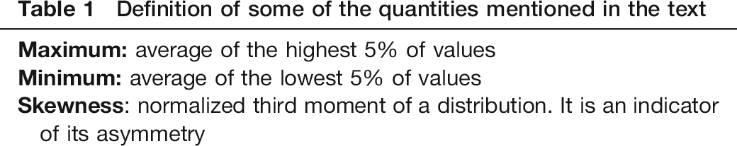
From each parametric map, a set of statistics was obtained from the tumor ROIs previously described. For nCBV and FM maps, the statistics computed were the median, minimum (average of the lowest 5% of values), maximum (average of the highest 5% of values), entropy, kurtosis, and skewness of the parameter distribution. For TTP values, the statistics calculated were entropy, kurtosis, and skewness (Table 1).

Table 1

Definition of some of the quantities mentioned in the text

Maximum: average of the highest 5% of values

Minimum: average of the lowest 5% of values

Skewness: normalized third moment of a distribution. It is an indicator of its asymmetry

S k e w n e s s = \frac{Σ_{i = 1}^{N} {(x_{i} - \bar{x})}^{3}}{(N - 1) s^{3}}

[1]

Kurtosis: normalized fourth moment of a distribution. It is an indicator of how peaked the distribution is

K u r t o s i s = \frac{Σ_{i = 1}^{N} {(x_{i} - \bar{x})}^{4}}{(N - 1) s^{4}}

[2]

with

s = \sqrt{\frac{Σ_{i = 1}^{N} {(X_{i} - \bar{X})}^{2}}{(N - 1)}}

Entropy: a measure of uncertainty of a random variable, defined as

E n t r o p y = - Σ_{i = 1}^{N} (p (x_{i}) \log_{2} p (x_{i}))

[3]

where p(x_i) can be estimated by computing the sample histogram

An estimate of the tumor volume was also computed for each tumor by multiplying the number of voxels in the tumor ROI by the voxel volume.

Further, in order to assess differences in the level of enhancement between tumors of different grade, maximum relative enhancement was calculated as the average of the highest quartile of (S_post/WM_post-S_pre/ WM_pre) in the ROI encompassing the tumor. S_pre is the signal in the pre-contrast image, S_post the signal in the post-contrast image, WM_pre the average of the pre-contrast image signal in the white matter ROI and WM_post the average of the post-contrast image signal in the white matter ROI (which excluded voxels from the tumor region). A similar measure has been used previously (15), but in this case the average of the highest quartile was taken instead of the average of the full sample, because high values of enhancement were considered a more robust indicator of the presence or absence of tissue leakage.

Enhancement assessment

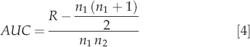
Taking maximum relative enhancement (estimated as described above) as independent variable, a logistic regression model was fitted to the assessment of presence or absence of enhancement made by the radiologist on a subsample of 43 of the subjects (16 grade II, 9 grade III and 18 grade IV). The area under the receiver-operating characteristic (ROC) curve (AUC) (28) was calculated to evaluate the validity of the maximum relative enhancement values as an automated approximation of the radiologists’ estimation. The AUC estimates the probability of a positive case (i.e. enhancement present) being assigned a higher value than a negative case. It can be computed with the formula:

A U C = \frac{R - \frac{n_{1} (n_{1} + 1)}{2}}{n_{1} n_{2}}

[4]

where R is the sum of the ranks of all the positive instances with regard to their value, and n₁ and n₂ the number of positive and negative instances, respectively. In addition, a threshold that minimized the error rate (number of mis-classifications/total cases when separating absence from presence of enhancement based on maximum relative enhancement values) was also computed.

Tumor grading variable selection

The design of a diagnostic system requires the definition of a model derived from previous independent observations. Cross-validation techniques are used to generalize prediction accuracy of a model or method (29) by splitting an available data-set into two parts: a training set, which is used to estimate the parameters of the predictive model, and a test set, on which the performance of the model is assessed. The process is repeated by partitioning the data-set multiple times, and summary statistics of the scores obtained with different training/test partitions are calculated. For each of the features introduced in the previous section (Table 2), a logistic regression model (30) was fitted to a balanced, random sample of 15 HGG (high-grade gliomas, grade III + grade IV) and 15 LGG (low-grade gliomas, grade II). The fitted model was used to classify the remaining 44 subjects and the AUC was calculated. This procedure was repeated 1000 times in a random subsampling design, to obtain median AUC (mAUC) and standard deviation. Next, a forward stepwise selection algorithm was applied: for all possible combinations of two features including the feature with highest mAUC value, mAUC was computed in the same way as for the single features. Similarly, for each n features, the combination of n features with highest mAUC was searched among all combinations of n features that included the combination of n-1 features with highest mAUC. A flowchart describing the entire procedure is shown in Fig. 2.

Fig. 2

Overview of the procedures applied to select the optimal combination of features, assessed using a logistic regression model. The scores computed were AUC (area under the curve), TRER (training error rate), TER (test error rate), SN (sensitivity), and SP (specificity)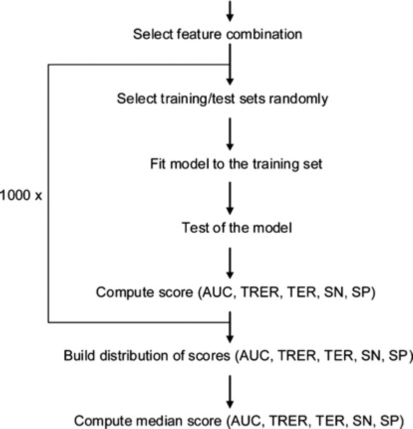

Table 2

Evaluated features with their corresponding area under the ROC curve values

Feature	Grade II vs. III (5 HGG-5 LGG) mAUC (SD)	Grade II vs. III + IV (5 HGG-5 LGG) mAUC (SD)	Grade II vs. III + IV(15 HGG-15 LGG) mAUC (SD)
Median nCBV	0.68(0.17)	0.82 (0.07)	0.82 (0.04)
Maximum nCBV	0.70(0.16)	0.81 (0.08)	0.81 (0.04)
Minimum nCBV	0.56(0.13)	0.54 (0.08)	0.52(0.10)
nCBV Entropy	0.73(0.14)	0.87 (0.04)	0.87 (0.04)
nCBV Kurtosis	0.48 (0.08)	0.76(0.10)	0.76 (0.06)
nCBV Skewness	0.49(0.11)	0.80(0.11)	0.80 (0.05)
Median FM	0.45(0.12)	0.71 (0.16)	0.72 (0.07)
Maximum FM	0.56(0.17)	0.79(0.14)	0.80 (0.05)
Minimum FM	0.58(0.15)	0.56 (0.09)	0.56(0.10)
FM Entropy	0.54(0.14)	0.74(0.14)	0.75 (0.05)
FM Kurtosis	0.62 (0.15)	0.49 (0.05)	0.47 (0.06)
FM Skewness	0.43(0.10)	0.51 (0.05)	0.51 (0.07)
TTP Entropy	0.46 (0.06)	0.50 (0.04)	0.48 (0.06)
TTP Kurtosis	0.54(0.13)	0.51 (0.05)	0.49 (0.08)
TTP Skewness	0.57(0.13)	0.48 (0.03)	0.46 (0.06)
Max RelEnhancement	0.76 (0.13)	0.94 (0.01)	0.94 (0.02)
ROI volume	0.59(0.16)	0.53 (0.07)	0.52 (0.09)

mAUC = median area under the ROC curve, SD = standard deviation, nCBV= normalized cerebral blood volume, FM = first moment of the first-pass-curve, TTP = time-to-peak, HGG = high-grade glioma, LGG = low-grade glioma

The analysis was repeated fitting the logistic regression model to random samples of five HGG and five LGG and subsequently testing it on the remaining 64 subjects. Finally, the aforementioned scheme was applied to the sub-sample of patients with grade II and III tumors, using five HGG and five LGG for the training sets and testing the fitted models on the remaining 30 subjects every time.

A logistic regression model was trained on the balanced random samples using the combination of features with the highest mAUC, and a threshold that minimized misclassifications in the training set was found. The trained model was applied using the threshold to classify the samples in the test set. This process was repeated 1000 times to construct an estimated distribution of training error rate (misclassified elements in the training set/total number of elements in the training set), test error rate (mis-classified elements in the test set/total number of elements in the test set), sensitivity, and specificity of the method.

Survival time analysis

Maximum relative enhancement was binarized using the threshold obtained (see ‘Data analysis’ section), and the other features were rescaled to have zero mean and a standard deviation equal to one. A Cox proportional-hazards regression model (31) was used to analyze the survival time of the 74 patients. This model describes changes of the hazard (risk of terminal event, death in this case) over time, assuming the following relationship for a set of features x_i, i = 1..n.

h (t) = \exp (α (t) + β_{1} x_{1} + β_{2} x_{2} + \dots + β_{n} x_{n})

[5]

h(t) is the hazard, x_i the features involved in the model, and a(t), β_i the parameters that need to be estimated. The parameters β_i are indicative of the magnitude of the effect of each corresponding feature, since one unit of a feature x_i produces a change equal to exp(β_i) in the value of the hazard h(t).

A forward stepwise selection procedure (as in the ‘Tumor grading variable selection’ section) was used to select the best composite model (i.e. feature combination) according to the Akaike Information Criterion (AIC) (32), which depends on the number of parameters and the value of the likelihood for the parameter estimates {β₁,…,β_n} which maximize such likelihood. The AIC can be used as a principle for model comparison because it measures the goodness of fit of a model in trade-off with its complexity (number of parameters included). Models with lower AIC are favored over models with higher AIC. The selection procedure calculates the AIC for each of the single-feature models and selects the one which ranks highest. With the selected feature, all the possible double-feature models containing it are ranked, and the new model is selected if the AIC is higher than for the chosen single-feature model. Only models with no more than two features were considered in order to avoid overfitting.

Intervals between pre-contrast and post-contrast scans

An independent samples t-test was performed for the intervals between pre-contrast and post-contrast scans (from the start of the DSC acquisition to the start of the T1-weighted post-contrast scan) to test for a significant bias between intervals from LGG and HGG patient acquisitions. This was done to ensure that maximum relative enhancement was a valid measure to be included in the analysis explained in the previous sections.

All the analyses in this section were done using R (33) and MATLAB (Mathworks, Inc., Natick, MA, USA).

Results

Histological analysis

Histopathological analysis of the biological samples revealed 30 grade II, 10 grade III (3 anaplastic astrocytomas, 3 anaplastic oligodendrogliomas, 4 anaplastic oligoastrocy-tomas), and 34 grade IV tumors according to the WHO classification of central nervous system tumors (2).

Enhancement assessment

The value of the AUC for the logistic regression model on the 43 subject subsample was 0.96, revealing strong agreement between maximum relative enhancement and the assessment of absence or presence of enhancement done by the radiologist. Fig. 3 shows a boxplot illustrating how maximum relative enhancement values are distributed in relation to the assessment by the radiologist. A threshold of 0.42 was found to give the lowest error rate, equal to 0.07 (3 tumors misclassified by the logistic model, out of 43), corresponding to a sensitivity of 0.86 and a specificity of 0.95.

Fig. 3

Assessment by the radiologist (absence or presence of contrast enhancement) vs. maximum relative enhancement. Tumors with presence of enhancement as evaluated by the radiologist tend to have higher maximum relative enhancement values than those with absence of contrast enhancement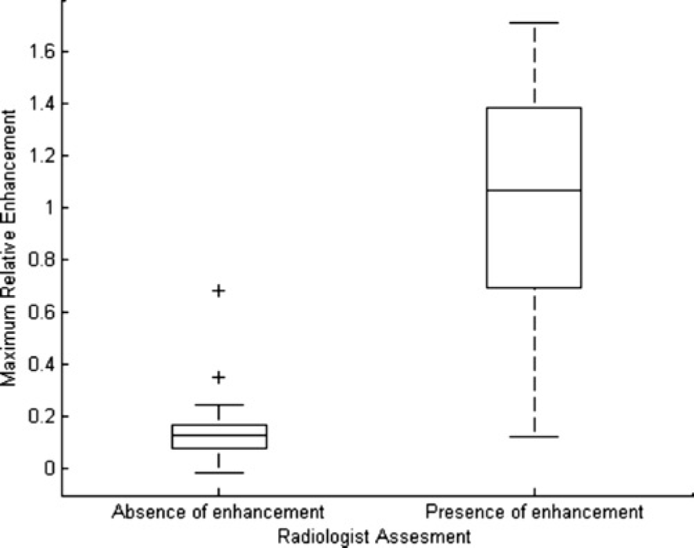

Tumor grading variable selection

Table 2 shows mAUC(SD) for each of the features of the set when considered separately, and the three analysis scenarios examined (II vs. III, training with 5 HGG-5 LGG; II vs. III + IV, training with 5 HGG-5 LGG; II vs. III + IV, training with 15 HGG-15 LGG). The single feature with highest mAUC was maximum relative enhancement.

For the three analysis scenarios considered, the combination of two features with highest mAUC was maximum relative enhancement + FM kurtosis. By far, the main contribution (increase in mAUC when adding a new feature to the model) was due to the maximum relative enhancement. In the case of three or more features, the gain in mAUC for an additional feature (<1%) was below variations in mAUC due to sampling differences.

Table 3 displays the median values and standard deviations for AUC, training error, test error, sensitivity, and specificity for the combination of maximum relative enhancement + FM kurtosis. Training the model with 5 HGG-5 LGG instead of 15 HGG-15 LGG yielded very similar median values for AUC, training error, test error, sensitivity, and specificity, but increased standard deviation. Fig. 4 a-e depict the distribution of these values for the scenario II vs. III + IV (solid lines), when the training was done with 5 HGG-5 LGG. A rather high predictive power was achieved when the whole sample was used (mAUC = 0.96), but notably lower values (mAUC = 0.82) were obtained when grade IV tumors were excluded. Fig. 4f shows the whole sample in the space spanned by the variables maximum relative enhancement and FM kur-tosis. Grade IV tumors presented in general with higher values of enhancement and higher FM kurtosis than grade II tumors. A similar trend was seen for grade III tumors, but with a much larger overlap with grade II tumors, resulting in a reduced predictive performance.

Fig. 4

(a) Calculated distribution of area under the ROC curve (AUC); (b) training error rate; (c) test error rate; (d) sensitivity; and (e) specificity. All figures relate to the cases grade II vs. grade III (solid line) and grade II vs. grade III + IV (dotted line), in both situations using a training set with 5 HGG and 5 LGG and a test set with the remaining cases, reshuffling the sets 1000 times. Discrimination power was poorer when grade IV tumors were excluded, since grade III tumors present with values of maximum relative enhancement + FM kurtosis similar to those of grade II tumors, as can be seen in Fig. 4f. The lines on Fig. 4f indicate class boundaries for the 1000 thresholded logistic models (training sets with 15 HGG and 15 LGG; solid line = mean boundary, dotted lines = standard deviation)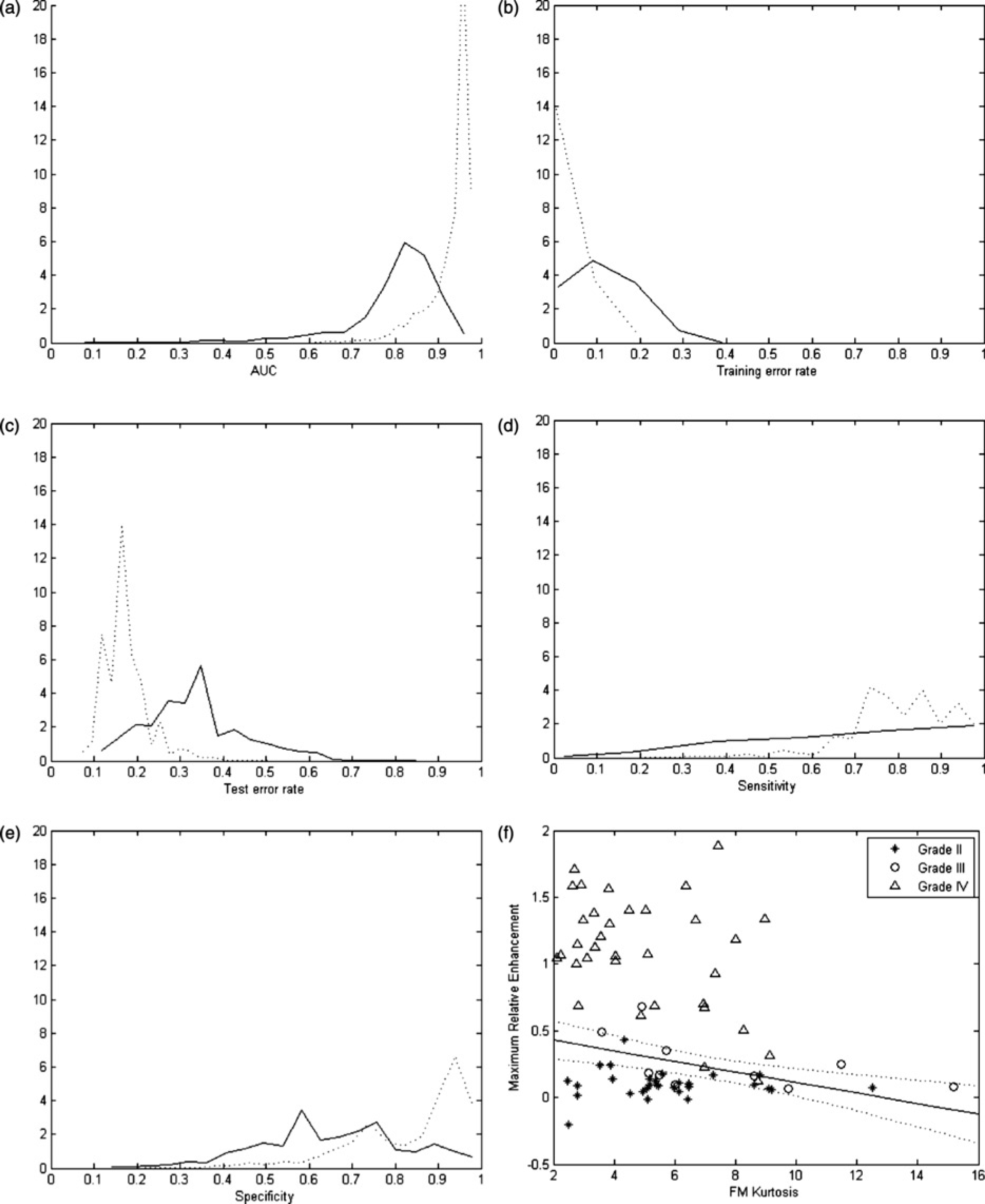

Table 3

Combination of maximum relative enhancement + FM kurtosis

AUC	0.82 (0.10)	0.95 (0.06)	0.96 (0.02)
Training error rate	0.10 (0.09)	0.00 (0.05)	0.07 (0.04)
Test error rate	0.33 (0.11)	0.17 (0.06)	0.14 (0.04)
Sensitivity	0.80 (0.26)	0.82 (0.12)	0.86 (0.08)
Specificity	0.68 (0.17)	0.88 (0.15)	0.87 (0.12)

Median values for AUC (area under the ROC curve), training and test error rates, sensitivity, and specificity. Standard deviations between parentheses. The class boundaries for the thresholded logistic models are shown in Fig. 4f HGG = high-grade glioma, LGG = low-grade glioma, FM = first moment of first-pass curve

Survival time analysis

The model chosen by the selection algorithm, ranked with the lowest AIC, was the one formed by binarized maximum relative enhancement alone, with P < 0.0001. The corresponding parameter estimate β = 1.72 (±0.39), rendered an exp (β) = 5.58 times increase in hazard of death in presence of enhancement.

The AIC value for a model including only the grade was equal to 241.55, whereas that for binarized maximum relative enhancement was 254.77, which points out the former as being more informative than the latter with respect to prediction of survival time. This effect can be appreciated in Fig. 5a and b, which show the corresponding boxplots (including only the 35 deceased patients and the 13 patients that survived longer than the longest-surviving deceased patient). The resulting Kaplan-Meier survival curves are plotted in Fig. 5c and d.

Fig. 5

(a) Boxplot of survival time vs. grade (HGG = high-grade glioma, LGG = low-grade glioma). (b) Boxplot of survival time vs. presence or absence of contrast enhancement (assessed as binarized maximum relative enhancement). The plots include only the 35 deceased patients and the 13 patients that survived longer than the longest-surviving deceased patient. (c, d) Corresponding Kaplan-Meier survival curves, including the whole study sample (74 patients). In Fig. 5c the population is segregated in 44 HGG and 30 LGG, whereas in Fig. 5d the population is segregated in 34 enhancing vs. 40 non-enhancing tumors

Intervals between pre-contrast and post-contrast scans

Intervals between pre-contrast and post-contrast scans were available for 72 of the 74 patients; in the remaining two subjects the DSC acquisition and the T1-weighted post-contrast images were acquired on different dates. Average time between T1-weighted pre- and post-contrast acquisitions was 309.86±315.34 seconds for LGG and 372.33±357.33 seconds for HGG, with no significant difference between low and high grades (P = 0.45 on independent samples t-test).

Discussion

In this study we assessed the value of a set of contrast MR-derived tumor features for glioma grading and survival time prediction. Our goal was to select the subset of features which provided most diagnostic information according to the defined criteria. Perhaps paradoxically, from all the features considered in this study, some of which entailed a sophisticated analysis, presence/absence of contrast enhancement proved to be the best marker of malignancy in spite of the high values of mAUC obtained for some of the DSC derived parameters (0.88 for CBV entropy), in agreement with previous studies (4, 13). The presence of contrast enhancement reveals the existence of transendothelial leakage due to augmented vascular permeability and anomalous blood-brain barrier function, which reportedly occur in advanced stages of tumor progression (34). The minor contribution of FM kurtosis would indicate a slight tendency for more dispersed transit times concurrent with absence of enhancement in the case of low-grade gliomas, as Fig. 4f shows. Moderately high sensitivity and very elevated specificity values were achieved when using the logistic regression model to grade the tumors from the MR-derived measurements, suggesting susceptibility to false-negatives predominantly. Adding other measures did not improve prediction accuracy for the grading.

The best survival predictor was also the presence or absence of enhancement. In the context of the model used, presence of enhancement would increase the hazard of death by more than a factor of 5. The effect is apparent when plotting the survival curves for the population segregated by presence or absence of enhancement (Fig. 5d). However, histological diagnosis still provided a better separation than contrast enhancement as seen in Fig. 5c, which would indicate that histology is a more reliable survival predictor than enhancement and hence than any of the parameters tested.

Several methodological issues need to be discussed. Although the sample has a considerable size, it is unbalanced with respect to grade III gliomas, with only 10 cases, compared to 30 (grade II) and 34 (grade IV) tumors. This fact has led to the high performance of enhancement analysis in terms of differentiation between low- and high-grade tumors, since glioblastomas (grade IV) typically show enhancement, whereas anaplastic gliomas (grade III) often show no enhancement (15). Indeed, when narrowing down the sample to include only grade II and grade III gliomas, lower discrimination power was obtained. A recent study that explored enhancement-related measures (14) also found good discrimination between grades II and IV, but not between grades II and III. Due to the few available cases of grade III tumors, only 10 subjects were used in the training data-set, but the estimates should still be accurate enough, since reducing the training data-set from 30 to 10 cases did not change substantially the estimates for the whole sample.

Concerning the manual segmentation of the tumor ROIs, tracing was done in conformity with former studies. An automated method of delineation of the tumor mass would yield more reproducible results, but no satisfactory automated method was available, and the implementation of such a method was beyond the scope of this study.

The fact that the time between pre- and post-contrast acquisitions was not the same for all patients implies that the maximum relative enhancement has to be interpreted as a measure of presence rather than continuous amount of leakage. Ideally, the pre- to post-contrast acquisition interval should be constant across subjects. This would have made it possible to establish correlations with other parameters. This not being the case, the dynamics of the contrast enhancement could confound physiological differences, and therefore an empirically found threshold was used in order to binarize the measure and include the parameter in the analysis. It also needs to be remarked that the DSC sequence was acquired using a double dose of contrast agent, and as a consequence the post-contrast T1-weighted scans also had a double dose. The results may therefore not be comparable to studies done using a single dose.

In conclusion, after systematically comparing a collection of structural and perfusion-related MRI parameters and assessing their diagnostic value in terms of tumor grading and survival prediction, we have shown that presence or absence of contrast enhancement was the best predictor among the statistical quantities investigated. In view of the current lack of standardization of DSC and dynamic contrast-enhanced (DCE) methods, measures as the maximum relative enhancement have the advantage of being simple and robust, but our observations point toward the need to consider also more elaborated estimates of permeability in future investigations.

Footnotes

Acknowledgements

We thank David Scheie, from Rikshospitalet, Oslo University Hospital (Oslo, Norway), for contributions to this work.

Conflict of interest: None.

References

Schwartzbaum

, Fisher

, Aldape

Epidemiology and molecular pathology of glioma. Nat Clin Pract Neurol 2006; 2: 494–503.

Louis

, Ohgaki

, Wiestler

Astrocytic tumours and Oligodendroglial tumours. WHO classification of tumours of the central nervous system. 4th edn. Astrocytic tumours and Oligodendroglial tumours WHO classification of tumours of the central nervous system 4th edition. Lyon: IARC, 2007: 8–11.

Law

, Yang

, Wang

Glioma grading: sensitivity, specificity, and predictive values of perfusion MR imaging and proton MR spectroscopic imaging compared with conventional MR imaging. Am J Neuroradiol 2003; 24: 1989–98.

Law

, Young

, Babb

Gliomas: predicting time to progression or survival with cerebral blood volume measurements at dynamic susceptibility-weighted contrast enhanced perfusion MR imaging. Radiology 2008; 247: 490–8.

Shin

, Lee

, Kwun

Using relative cerebral blood flow and volume to evaluate the histopathologic grade of cerebral gliomas: preliminary results. Am J Roentgenol 2002; 179: 783–9.

Sugahara

, Korogi

, Shigematsu

Value of dynamic susceptibility contrast magnetic resonance imaging in the evaluation of intracranial tumors. Top Magn Reson Imaging 1999; 10: 10.

Jenkinson

, Du Plessis

, Walker

Advanced MRI in the management of adult gliomas. Br J Neurosurg 2007; 21: 550–61.

Simon

, Schramm

Surgical management of intracranial gliomas. Recent Results Cancer Res 2009; 171: 105–24.

Graif

, Bydder

, Steiner

Contrast-enhanced MR imaging of malignant brain tumors. Am J Neuroradiol 1985; 6: 855–62.

10.

Ostergaard

Cerebral perfusion imaging by bolus tracking. Top Magn Reson Imaging 2004; 15: 3–9.

11.

Cha S. Perfusion

imaging: basic principles and clinical applications. Magn Reson Imaging Clin N Am 2003; 11: 403–13.

12.

Law

, Young

, Babb

Histogram analysis versus region of interest analysis of dynamic susceptibility contrast perfusion MR imaging data in the grading of cerebral gliomas. Am J Neuroradiol 2007; 28: 761–6.

13.

Emblem

, Nedregaard

, Nome

Glioma grading using histogram analysis of blood volume heterogeneity from MR-derived cerebral blood volume maps. Radiology 2008; 247: 808–17.

14.

Mills

, Soh

, O'Connor

Tumour enhancing fraction (EnF) in glioma: relationship to tumour grade. Eur Radiol 2009; 19: 1489–98.

15.

White

, Zhang

, Kirby

Can tumor contrast enhancement be used as a criterion for differentiating tumor grades of oligodendrogliomas?

Am J Neuroradiol 2005; 26: 784–90.

16.

Law

, Oh

, Babb

Low-grade gliomas: dynamic susceptibility-weighted contrast-enhanced perfusion MR imaging- prediction of patient clinical response. Radiology 2006; 238: 658–67.

17.

Patankar

, Haroon

, Mills

Is volume transfer coefficient (K(trans)) related to histologic grade in human gliomas?

Am J Neuroradiol 2005; 26: 2455–65.

18.

Mills

, Patankar

, Haroon

Do cerebral blood volume and contrast transfer coefficient predict prognosis in human glioma?

Am J Neuroradiol 2006; 27: 853–8.

19.

Wolf

, Wang

Grading of CNS neoplasms using continuous arterial spin labeled perfusion MR imaging at 3 Tesla. J Magn Reson Imaging 2005; 22: 475–82.

20.

Hamstra

, Chenevert

, Moffat

Evaluation of the functional diffusion map as an early biomarker of time-to-progression and overall survival in high-grade glioma. Proc Natl Acad Sci USA 2005; 102: 16759–64.

21.

Pope

, Kim

, Huo

Recurrent glioblastoma multiforme: ADC histogram analysis predicts response to bevacizumab treatment. Radiology 2009; 252: 182–9.

22.

Zeng

, Liu

, Zhang

Noninvasive evaluation of cerebral glioma grade by using multivoxel 3D proton MR spectroscopy. Magn Reson Imaging 2011; 29: 25–31.

23.

Erb

, Elbayed

, Piotto

Toward improved grading of malignancy in oligodendrogliomas using metabolomics. Magn Reson Med 2008; 59: 959–65.

24.

Smith

, Jenkinson

, Woolrich

Advances in functional and structural MR image analysis and implementation as FSL. Neuroimage 2004; 23: 208–19.

25.

Boxerman

, Schmainda

, Weisskoff

RM.

Relative cerebral blood volume maps corrected for contrast agent extravasation significantly correlate with glioma tumor grade, whereas uncorrected maps do not. Am J Neuroradiol 2006; 27: 859–67.

26.

Friston

, Holmes

, Worsley

KJ.

Statistical parametric maps in functional imaging: a general linear approach. Hum Brain Mapp 1995; 2: 189–210.

27.

Schmainda

, Rand

, Joseph

Characterization of a first-pass gradient-echo spin-echo method to predict brain tumor grade and angiogenesis. Am J Neuroradiol 2004; 25: 1524–32.

28.

Obuchowski

NA.

Receiver operating characteristic curves and their use in radiology. Radiology 2003; 229: 3–8.

29.

Shao

Linear Model Selection by Cross-Validation. Journal of the American Statistical Association 1993; 88: 486–94.

30.

Hosmer

, Lemeshow

Applied logistic regression. 2nd edn. New York, NY: Wiley Interscience, 2000: 31–3.

31.

Cox

, Oakes

Analysis of Survival Data. London: Chapman and Hall, 1984:70–1.

32.

Akaike

A new look at the statistical model identification. IEEE Transactions on Automatic Control 1974; 19: 716–23.

33.

R-Development-Core-Team

: A Language and Environment for Statistical Computing. Vienna: R Foundation for Statistical Computing, 2008.

34.

Vajkoczy

, Menger

MD.

Vascular microenvironment in gliomas. J Neurooncol 2000; 50: 99–108.