Simulation of digital scan conversion for ultrasound systems using a digital signal processor

Abstract

B-mode ultrasound systems use digital scan conversion (DSC) to display data in a Cartesian coordinate system acquired in a polar coordinate format. Image quality depends on the quality of the interpolation algorithm applied to the unsampled pixels to avoid artefacts. In this paper, a warped distance-based adaptive bilinear interpolation technique with selective sampling is proposed and has been successfully simulated using a Texas Instruments (TI) digital signal processor series TMS320C64x+ cycle accurate simulator. The algorithm enhances both the detail in the different regions as well as preserving the smooth regions within the image, yielding better image quality with less computational complexity. Optimized implementation of the algorithm supports software pipelining. Additionally, the approach speeds up the computation by utilizing the ability of very long instruction word processor to perform multiple operations in parallel. The experimental results show that the DSC is capable of supporting 83 frames per second without sacrificing the image quality for a raw input image of size, 512 × 256 scanned with an angle of 58° and output video graphics array (640 × 480) display.

Keywords

Ultrasound digital scan conversion digital signal processors interpolation realtime systems VLIW

Digital scan conversion (DSC) is an indispensable component of B-mode ultrasound systems. DSC is required to display a two-dimensional image of the tissue structure. The image is formed by combining the series of pulse-echoes in the individual lines of sight of the transducer. The signal is sampled with constant step size in both angle and radius.¹ The sampling space of a conventional pulse-echo digital ultrasound sector scanner is in polar coordinates. However, the display space used by digital monitors is in Cartesian coordinate, which necessitates a coordinate transformation. However, coordinate transformation requires the inverse tangent to determine the scanning angle and square root of sum of the squares of the x and y coordinates to decide the pixel positions along the radius. This involves a high level of computation, which requires the use of dedicated hardware for realtime implementation.² Furthermore, interpolation is required for the undersampled space to avoid artefacts like Moiré effects.³ When samples are mapped onto the display device, the pixels which are located in between two scan lines are not assigned a value. This is apparent in the case of sector scanning as pixels far from the transducer face will have less probability of being associated with a sample. Therefore, some interpolation mechanism has to be incorporated during the coordinate transformation. To obtain continuous representation of a sampled image, it can be convolved with a sinc function. Then by resampling in the Cartesian coordinate system an ideal scan-converted image can be obtained.⁴ Owing to the infinite extent of the sinc function, realtime implementation is not feasible, which necessitates a more accurate and faster algorithm.

Numerous interpolation algorithms have been proposed and examined by numerous researchers^2–14 for approximate DSC. Among them, the nearest-neighbourhood interpolation (NNI) substitutes every pixel value with the nearest pixel in the spatial domain.⁷ NNI is very fast and can be easily implemented by maintaining a lookup table for the x and y coordinates for mapping to both the sample index and the scan line number. NNI works well for a large number of scan lines. For low sampling rate, it, however, produces artefacts in the images, they appear both blocky and quantized due to pixel quantization, referred to as an aliasing effect. Linear interpolation was used by Richard and Arthur⁸ with oversampled echo data and Fritsch et al. ⁹ used a selective sampling technique to acquire the data at specific points. Chang et al. ¹⁰ used a linear interpolation algorithm implemented with single Field Programable Gate Array (FPGA) (Stratix EP1S60F1020C6, Altera Corporation, San José, CA, USA) as a simplified version of bilinear interpolation, this FPGA had a speed of 400 frames per second (fps) for an image size of 256 × 256. However, in order to produce good-quality images the algorithm needed a sampling rate at least four times higher than the Nyquist rate for the baseband component. Software implementation of realtime DSC using bilinear interpolation has been used by Wang et al. ⁶ This DSC technique performs at a speed of 67 fps for an input image size 256 × 128 and output image size 512 × 512. Bilinear interpolation is the best algorithm in terms of speed and accuracy;¹⁰ however, the hardware implementation of this may be costly due to its complex operations. Also the bilinear interpolation algorithm necessitates at least four data-fetch operations, involving complex buffer management. Realtime bilinear interpolation can be implemented in a Spartan-II FPGA at a speed of 60 fps.¹¹ Several restrictions associated with this device to implement bilinear interpolation in hardware are discussed by Gribbon and Bailey.¹¹ In order to increase the operating speed of DSC with bilinear interpolation the design has to be much more sophisticated, which again increases the cost of implementation. A cubic convolution interpolation algorithm gives better enhancement, although a blurring effect tends to be present, especially in the edge regions.¹² A filtering technique based on cubic convolution has been used for scan conversion implemented in Texas Instruments (TI's) digital signal processor (DSP) C6416 chip by Hou and Liu.¹³ Interpolation with cubic spline has been found to yield images of satisfactory quality.¹⁴ DSC in frequency domain using Fourier transform has been proposed by Ahn et al. ⁵ However, all these algorithms are computationally intensive.

Various interpolation algorithms have appeared in the literature^15–18 to enhance the detail or edges within images. Linear interpolation with warped distance has been implemented by Ramponi, 1999.¹⁵ Warped distance-based adaptive bilinear, bicubic and cubic spline interpolation methods have been discussed by Hadhoud et al. ¹⁶ These adaptive interpolations are dependent on the weighting of the pixels participating in the interpolation in a space variant manner which results in enhanced edges. A combined approach of adaptive warp distance-based cubic interpolation and Kringing interpolation-based scan conversion is explained by Ma et al. ¹⁹; the algorithm described is not suitable for realtime dedicated hardware implementation due to its intense computation. Except for the selective sampling described by Fritsch et al.,⁹ all the above-mentioned methods use uniform sampling of polar spatial domain – this selective sampling facilitates low levels of computation.

This paper introduces a hybrid warped distance-based adaptive bilinear interpolation with a modified selective sampling algorithm implemented in a TI's low-cost DSP for high-speed DSC. This can produce B-mode images of video graphics array (VGA) (640 × 480) size at the rate of 83 fps. This interpolation algorithm enhances both edges and detailed regions within the image with low computation requirements while preserving the smooth regions within the image. For the sake of high speed, the algorithm has been designed and optimized to support software pipelining and instruction level parallelism available in DSP. The quality of the produced image is much better than that of NNI, linear interpolation and bilinear interpolation and the computational complexity is less than that of cubic convolution, bicubic interpolation and cubic spline interpolation methods.

The remainder of this paper is organized as follows. The next section reviews warped distance-based adaptive bilinear interpolation and the selective sampling technique on which the proposed algorithm is based. The proposed DSC algorithm is presented in the third section. Software pipelined DSP implementation of the proposed DSC module is explained in the fourth section. Experimental results are presented in the penultimate section. Finally, the last section summarizes the concluding remarks.

Interpolation and selective sampling technique: theoretical background

In this section, we briefly review the warped distance-based adaptive bilinear interpolation¹⁶ and the selective sampling technique⁹ algorithms used in the proposed algorithm of DSC for the formation of ultrasound images.

Warped distance-based adaptive bilinear interpolation

If the samples are taken at a fixed frequency, one-to-one mapping hardly exists between the position of the sampled data and the locations of pixels on the display. Therefore, some form of interpolation must be performed to generate the unmapped pixels. Bilinear interpolation is one of the most widely used interpolation algorithms.

Let x be the coordinate value to be interpolated and I(x _i) be the available data. Assuming that x _i and x _i+1 are the nearest neighbours of x, the distance between x and its neighbours can be given as

The simple bilinear interpolation algorithm can be written as

Two-dimensional bilinear interpolation can be implemented by applying Eq. (3) first along the rows and then along the columns. Warp distance interpolation is introduced to sharpen the edges. It can be estimated using the following equation as explained by Ramponi:¹⁵

where A _i refers to the asymmetry of the data in the neighbourhood of x and is defined as

For ultrasound images, the pixels are of 8 bit and L = 256. L is known as the scaling factor which controls the value of A _i ∈ [−1,1].

The parameter τ controls the intensity of warping and may be equal to one or two. In the interpolation mechanism, warping prevents the blurring of edges.

The adaptive bilinear interpolation function can be defined as:

where

and

The symbol λ is a constant which lies in between one and five.¹⁶ This constant λ regulates the intensity of weighting used for neighbouring pixels.

The selective sampling technique

The resolution of ultrasound information is generally higher in the radial direction than that of the angular direction. The selective sampling technique (SST) exploits this fact by using a high sampling rate. Data flow is maintained by selecting samples which are used either for display or for interpolation process.⁹

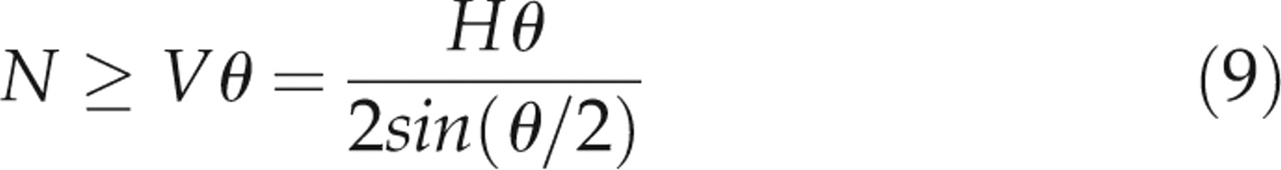
There should be one-to-one mapping between spatial domain pixels and pixels on the display, which implies that a huge number of scan lines need to be interpolated. The order of scan lines can be obtained from θV ²/2, where H × V is the size of the display and θ is the scan angle in radian. If the sampling rate is high enough, a smaller number of scan lines can also provide a good result, which can be explained by the relation given below:

When N scan lines are uniformly distributed over a sector of θ radian and maximum acceptable distance from any pixel to the scan line is d, then all the pixels up to a radius r _k have distance less than 2^k d to some scan line, where r _k can be given by the following equation:

The sector is divided into regions limited by radii [r _k, r _k+1], k = 1,2,… and 2^k−1 − 1 equispaced and virtual scan segments are introduced inbetween two adjacent real scan lines in every region k. The distance of a real or virtual scan line from any pixel will be less than d.

With Δ θ = θ/(N − 1), the maximum number of regions in a sector image is given by

where INT ₊(x) is the first integer greater than x.

Methods – proposed DSC algorithm

Interpolation algorithm

Even though the linear interpolation algorithm has the advantage of being easy to implement, it has the disadvantage of having the potential to cause smoothing at the edges and blurring detailed regions. The bilinear interpolation algorithm is linear interpolation along both the radial and the angular direction. So, with this method better image quality is obtained as compared with that of linear interpolation. The combination of warped distance with bilinear interpolation increases the sharpness of the images. With the further introduction of adaptiveness both edge and detail regions within the image are enhanced. So warped adaptive bilinear interpolation not only sharpens and enhances edges but also preserves the smooth regions. Amalgamation between the warped adaptive bilinear interpolation and the modified SST have the advantage of cutting down the computational complexity to a great extent. In Fritsch et al.,⁹ the sector is limited by the radius, ranging from r _k to r _k+1 where k = 1, 2 or 3 and the number of virtual scan lines introduced between two consecutive real scan lines in the region k are 2^k−1 − 1. However, this is not sufficient for reconstructing a good-quality scan converted image; therefore, in the proposed algorithm virtual scan lines are inserted in the region k which is redefined as 2^k−1 + 1 to satisfy the condition given in Eq. (10). The distance between two scan lines increases with the radial distance. The number of virtual scan lines introduced in regions has gradually been increased.

Cartesian conversion

For displaying each scan points in the output screen, the polar coordinates are to be converted to Cartesian coordinates utilizing an offset value for the fixed display screen with the following relationship:

The weighting coefficients for each pixel are computed depending on the asymmetry A _i at the pixel of interest.¹⁶ Followed by this, the image pixels are interpolated as shown in Figure 1a. In the next step, the pixel value for a particular (x,y) coordinate is computed using Eq. (12).

Figure 1
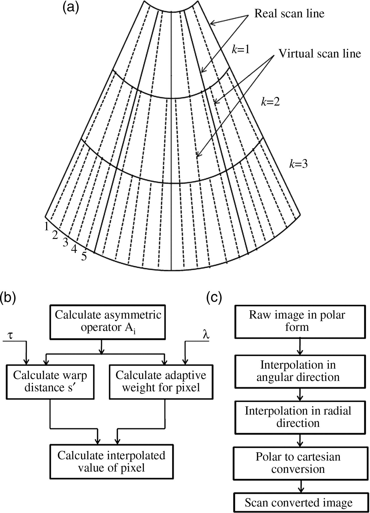
DSC methodology: (a) modiﬁed selective sampling technique, (b) interpolation methodology, (c) functional block diagram of DSC algorithm. DSC, digital scan conversion

The steps involved in the proposed scan conversion algorithm are described in the next section.

Proposed scan conversion algorithm

for all regions k (where k = 1, 2 or 3) such that do

Introduce 2^k−1 + 1 no. of equispaced virtual scan lines between two real scan lines

Introduce single virtual scan point between two adjacent real scan points on the same scan line in all regions

end for

for all virtual pixels with polar coordinate (r, θ) do

Calculate asymmetry A _i of pixel with neighbourhood known pixels

Calculate warp distance of pixel by A _i and distance from neighbourhood pixels

Calculate adaptive weights for the pixel of nearby known pixels with A _i

Calculate pixel value using warp distance based adaptive bilinear interpolation

end for

for all pixels in the polar coordinate do

(r, θ) to (x, y) is calculated

end for

The functional block diagram of the algorithm is shown in Figure 1b. Inref.¹⁶ constants τ and λ are used to control sharpness and enhancement of the image, respectively.

Parameter λ and τ

A parameter λ as described by Hadhoud et al. ¹⁶ is used as a controller of image enhancement, while a parameter τ is used to control the sharpness of the image. Variation of these two parameters (τ and λ) is tested with ultrasound image. Preferable values of λ and τ for the ultrasound images are 1 and 2, respectively.

According to the proposed algorithm, the raw image is divided into three regions. A single virtual scan line is introduced for region k = 1, three virtual scan lines in region k = 2 and five virtual scan lines in region k = 3. Again in all regions, a single virtual scan point is introduced in between two real scan points in radial direction. Figure 1c shows the orientation of newly inserted virtual scan lines. The introduced virtual points are then interpolated with a warped distance-based adaptive bilinear interpolation.

It is assumed that raw data are arranged in an array of M × N elements, where M is the number of scan points along every scan line, and N is the number of scan lines. If a scan point corresponds to (p,q) in raw image, p is the relative position of the scan point on that scan line and q is the index of the scan line. The radial distance of the scan point is determined by the relationship:

where R is the maximum radius on display.

The angle of the scan line is determined from the scan line number by the relationship:

where φ is the scan angle. The x and y coordinates of the pixel are then determined by the relation in Eq. (12). The offset adjustment is done such that the centre point remains at the horizontal centre of the screen. The value of θ is incremented by θ_inc, the angle of increment to access the next scan point in the same radius. The angle of increment can be calculated by the following relationship:

In the proposed scan conversion algorithm, as maximum of five virtual scan lines are introduced in between two real scan lines, in turn the effective number of scan lines, is increased to 6 × N − 5, where N is the initial number of scan lines. Similarly, the effective number of scan points in a single scan line is 2 × M − 1.

Methods – DSP implementation

The proposed algorithm is simulated using a TI DSP, series TMS320C64x+ cycle accurate simulator, which uses VelociTI™ (Texas Instruments, Dallas, Texas, USA) architecture and a high-performance advanced very long instruction word (VLIW).²⁰ The performance of the application depends on the compiler options, use of instructions, loop structures, etc.²¹ Implementation of the conditional branching using DSP is time intensive and also quite challenging for parallel processing.

The reasons why a loop can be disqualified for software pipelining are as follows:
The loop contains a call: an ‘If’ function call is within the loop;

The loop contains branching: if a loop contains a set of branch instructions or conditions in it.
For an optimized loop, the compiler is capable of doing fine grain scheduling of the functional units of each data path.²⁰ This is necessary to achieve the available instruction level parallelism. The algorithm is implemented avoiding conditions and function calls within the loop. Due to this, the compiler can generate parallel instructions to utilize the hardware resources maximally and exploit all the capabilities of the VLIW architecture.

The algorithm contains three major modules: (1) interpolation in angular direction (X-direction), (2) interpolation in radial direction (Y-direction) and (3) polar to Cartesian conversion. However, resizing of the raw image has to be performed before the interpolation is introduced. For writing optimized code, the algorithm has to be divided into independent functions so that there can be no condition or function call within loop of the code. How the structure of the processes from DSP-oriented view point is optimized is discussed in the next section.

DSC process division

Resizing

In order to introduce a virtual scan line in the radial direction and a virtual scan point in the angular direction, a resize function is used for resizing the raw image.

Interpolation

The raw image is divided into three regions as shown in Figure 1a. According to the referred algorithm, the number of scan lines introduced in successive three regions are one, three and five, respectively. As the radial distance increases, the separation between two adjacent scan lines is also increased. Understanding this fact, variable interpolation is done. Virtual scan line number 3 as in Figure 1a is present in all regions, i.e. k = 1, 2, 3. So, interpoleX3 function is defined to interpolate the points in the X-direction on the scan line. Virtual scan line numbers 1 and 5 are present in the region k = 2 and k = 3. So, interpoleX1_5 function is defined to interpolate the points in the X-direction on the scan lines. Virtual scan line numbers 2 and 4 are present only in the region k = 3. So, interpoleX2_4 function is defined to interpolate the points in the X-direction on the scan lines. Similarly, for interpolation in the Y-direction, independent functions are defined as shown in Table 1.

Table 1
Process division

Process Function

Resizing Resize Resize the image.

Interpolation in the X-direction interpoleX3 Interpolate the pixels on virtual scan line number 3 in all regions

interpoleX1_5 Interpolate the pixels on virtual scanline numbers 1 and 5 in region k = 2, 3

interpoleX2_4 Interpolate the pixels on virtual scanline numbers 2 and 4 in region k = 3

Interpolation in the Y-direction interpoleY3 Interpolate virtual scan points on scan line 3 in all regions

interpoleY1_5 Interpolate virtual scan points onscan lines 1 and 5 in region k = 2, 3

interpoleY2_4 Interpolate the pixels on virtual scanpoints numbers 2 and 4 in region k = 3

From polar-to-Cartesian conversion toCart3 Coordinate conversion of pixels on thereal scan lines and scan line 3

toCart1_5 Coordinate conversion of pixels onscan lines 1 and 5

toCart2_4 Coordinate conversion of pixels onscan lines 2 and 4

Polar-to-Cartesian conversion

For coordinate conversion of the pixels on all real scan lines and virtual scan line number 3, a function called toCart3 is defined. Polar-to-Cartesian conversion of the pixels on other scan lines is done by the functions shown in Table 1.

Avoiding floating point arithmetic

As TI's TMS320C64x+ cycle accurate simulator is a fixed point, floating point arithmetic is less efficient and also leads to inbuilt function (‘_fixfu’) called by the compiler for converting a single-precision floating point to an unsigned integer. So, for qualifying software pipelining floating point arithmetic has to be avoided. However, for each of the interpolation function asymmetry operator A _i, warp distance s′, adaptive weights a ₀ and a ₁ are to be calculated.¹⁶ Each of them involves floating point calculations. To avoid this problem, the variables involved in the calculations are left shifted and the accurate values of the interpolated pixels are then obtained. With this procedure single-precision floating point numbers are converted to the integers (with the required resolution). Since each of the intermediate variables is left shifted, and finally, the results are right shifted and correct values are substituted.

Again, the coordinate transformation functions involve floating point arithmetic because of sine and cosine values. The same methodology of shifting is used to maintain the software pipelining.

Using intrinsic

The C6000 compiler provides intrinsics, special functions which map directly to in-lined C64x+ instructions; these functions can be used for writing optimized code.²⁰ To calculate the asymmetric constant,¹⁶ absolute differences of the participating pixels are needed. The intrinsic _SUBABS4 is capable of performing the subtraction of two integers and thereby, return the absolute value. This intrinsic function is used for calculating the absolute difference of the pixels.

Calculating cosine and sine

The functions for coordinate conversion use Eq. (12). If sine and cosine library functions are called within the loop of coordinate conversion function the pipelining cannot be achieved. Moreover, to calculate sine and cosine values for a particular angle, DSP requires many clock cycles that can degrade the overall performance, whereas if the values are accessed from an array, the call function within the loop can be avoided as well as the clock cycles being reduced. So, sine and cosine values are calculated separately and stored in two different arrays as a look-up table (LUT) and thus qualify the software pipelining. The use of LUT also avoids calculating sin and cos of the same angle multiple times. Thus, repetition of the same calculation is avoided and the computation time is significantly reduced.

Avoiding conditions within a loop

The use of _SUBABS4 to calculate asymmetry A _i facilitates avoiding the condition to check the positive or negative differences for absolute difference of the participating pixels.

Pipeline design for interpoleX2_4

For the ease of understanding, implementation details of pipelined design for interpoleX2_4 are discussed here. This function is interpoleX2_4 and it is used to calculate the pixels in the X-direction on virtual scan line number 2 and 4. The function operates only in the last region, i.e. k = 3. The flow diagram of the function is shown in Figure 2. The following techniques are used for pipeline design:
To determine A _i, absolute difference of nearby real pixels is calculated by using _subabs4. To avoid division, we have taken A _i, as asymmetric constant left shifted by 8 bits;

Adaptive weights a ₀ and a ₁ are calculated by A _i, and intensity control constant λ. Warp distance s, with left shift of 20 bits is calculated by A _i and warping control constant τ is shifted by 12 bits;

The value of the interpolated pixel is calculated by using adaptive weight, warp distance and neighbourhood pixels with right shift of 28 bits to nullify above left shifts.

Figure 2
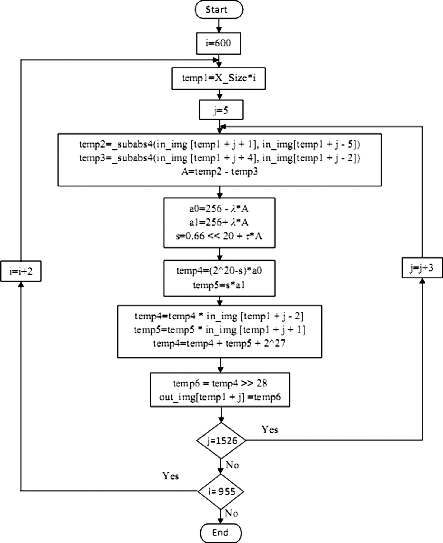
Flow diagram of interpoleX2_4

Using aforesaid methodologies, the compiler is able to generate the schedule for the functional units in each data path.²⁰ The assembly code snippets generated by the compiler for the function InterpoleX2_4 are given in Figure 3. It shows that there are multiple instructions like MV, SUB, MPYLI, ADD which are executed concurrently by the different functional units present in the two data paths using the VLIW architecture. The functional units .L1, .L1X, .S1X are of data path A and functional units .S2, .M2, .L2, .D2 are of data path B. Thus, we are able to utilize the hardware resources of DSP to the fullest extent taking advantage of its VLIW architecture. In this way, software pipelining is achieved by mapping the scan conversion algorithm into DSP.

Figure 3
Assembly code snippet

Results – simulation results

DSP TMS320C64x+ manufactured by TI is used to evaluate the performance of the proposed DSC algorithm. Simulations were performed on a cycle accurate simulator²⁰ by setting operating equal to 600 MHz. The algorithm was tested with raw ultrasound images with polar coordinates. The raw images were acquired on a GE's Logiq 5 ultrasound system using a 4C phased array probe (Make and Model: GE (GE Research Park, Wisconsin, USA), 4C, FoV: 58° and radius of 0.127 meter). On each scan line the same number of samples were picked-up and were stored as a raw image in a memory of size 512 × 256. The output display size was VGA (640 × 480).

First the bilinear and bicubic interpolation mechanisms were compared with warped distance-based adaptive bilinear interpolation¹⁶ by applying them on down-sampled ‘Mandrill and Cameraman’ images. These images were chosen as they have a large number of edges. The low-resolution images were obtained by down-sampling the images by a factor of two both in the vertical and horizontal directions. The original images of size 512 × 512 were down-sampled to a size of 256 × 256 to get low-resolution images. These images were brought back to their original resolutions using different interpolation techniques and the resultant images are shown in Figures 4 and 5. The mean-squared error (MSE), peak signal-to-noise ratio (PSNR), figure of merit (FOM) and edge-keeping index (EKI) values of the interpolated images were calculated with respect to the original images (See Appendix for further details.). The MSE and PSNR comparison results are shown in Table 2. The FOM and EKI comparison results are shown in Table 3. The results show that the warped distance-based adaptive bilinear interpolation technique yields better image quality particularly with respect to the MSE and PSNR parametric values. The results in Table 3 show that the warped adaptive bilinear interplation technique performs better than the bilinear interpolation with respect to edge preservation.

Figure 4
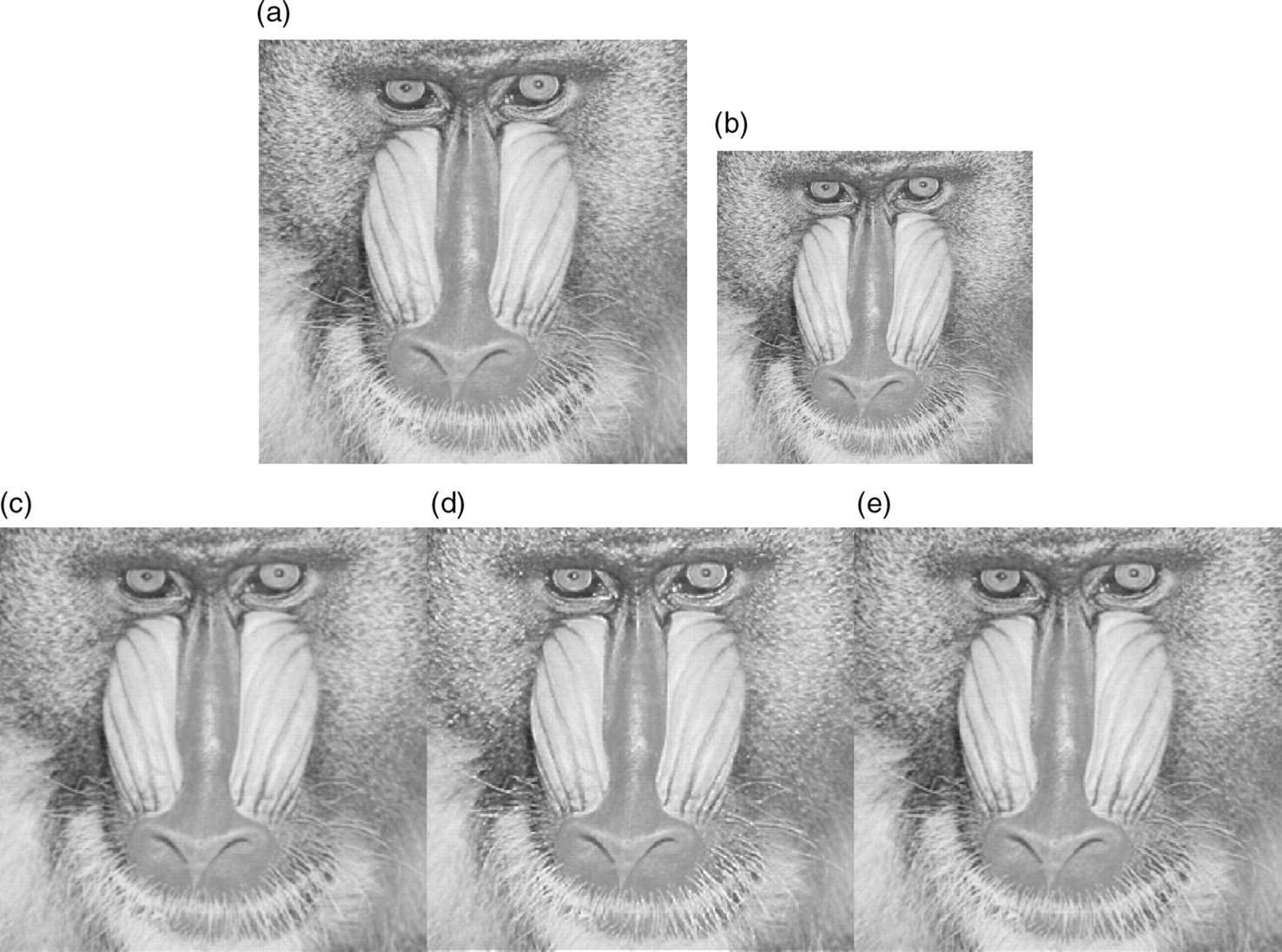
Interpolation on Mandrill: (a) original image, (b) down-sampled image (c) bilinear interpolation, (d) warped adaptive bilinear interpolation and (e) bicubic interpolation

Figure 5
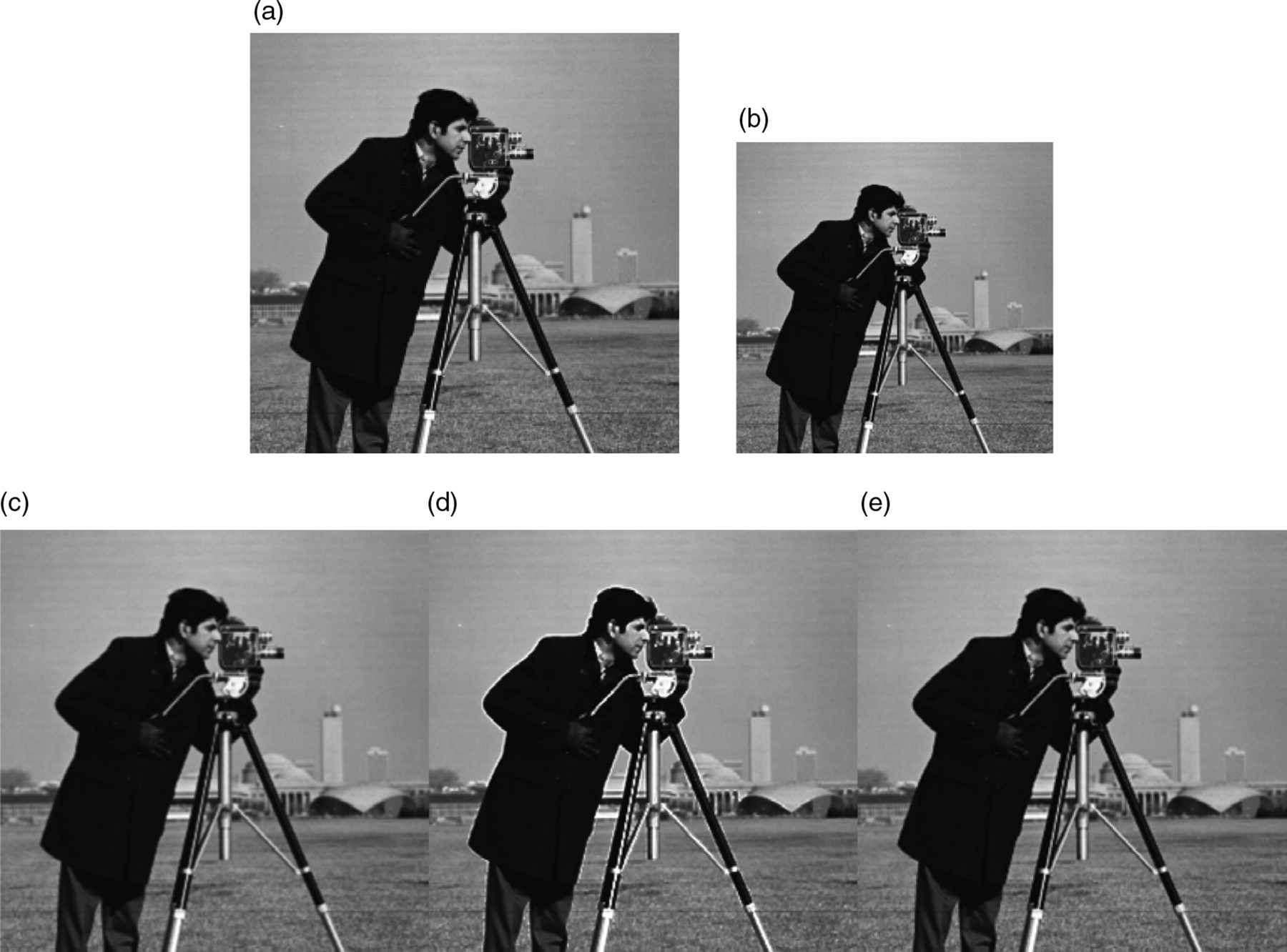
Interpolation on Cameraman: (a) original image, (b) down-sampled image (c) bilinear interpolation, (d) warped adaptive bilinear interpolation and (e) bicubic interpolation

Table 2
MSE and PSNR comparison

Interpolation algorithm MSE PSNR (dB)

Mandrill Cameraman Mandrill Cameraman

Bilinear interpolation 39.07 15.13 32.21 36.33

Bicubic interpolation 36.53 13.15 32.50 36.93

Warped adaptive bilinear interpolation 34.97 11.91 32.69 37.36

MSE, mean-square error; PSNR, signal-to-noise ratio

Table 3
FOM and EKI comparison

Interpolation algorithm FOM EKI

Mandrill Cameraman Mandrill Cameraman

Bilinear interpolation 0.9931 0.9964 0.7150 0.4564

Bicubic interpolation 0.9935 0.9978 0.8988 0.6210

Warped adaptive bilinear interpolation 0.9936 0.9979 0.8845 0.5924

FOM, figure of merit; EKI, edge keeping index

DSC with bilinear and bicubic interpolations implemented in MATLAB were compared with the proposed algorithm (λ = 1 and τ = 2) and the results are shown in Figures 6 and 7. The results demonstrated that the proposed DSC mechanism enhances the edges, the detail regions while preserving the smooth regions. The comparison of the computational complexity in terms of addition and multiplication is shown in Table 4; in this table, P = (N − 1)(2M − 1) and Q = N(M − 1), where the size of the raw image is M × N. It can be observed that the complexity of the proposed interpolation mechanism is much less than that of the cubic interpolation.

Figure 6
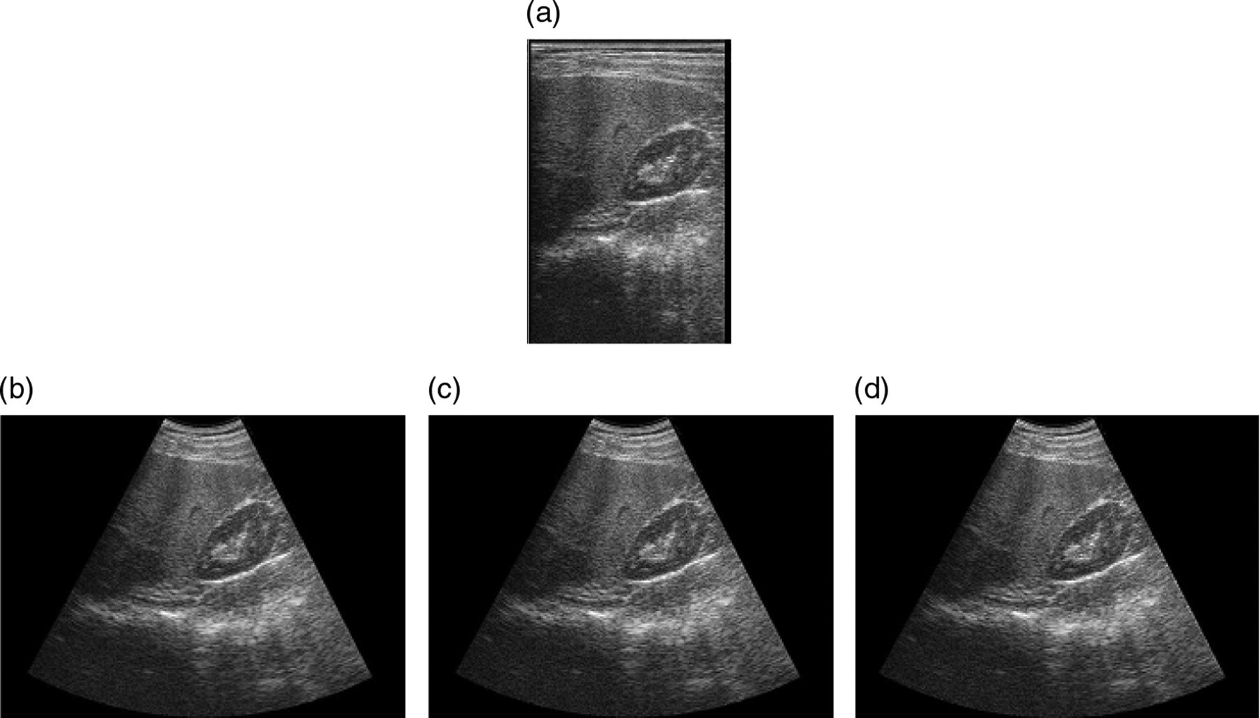
DSC of raw data I: (a) raw image, (b) bilinear interpolation, (c) bicubic interpolation and (d) proposed algorithm. DSC, digital scan conversion

Figure 7
DSC of raw data II: (a) raw image, (b) bilinear interpolation, (c) bicubic interpolation and (d) proposed algorithm. DSC, digital scan conversion

Table 4
Comparison of complexity

Interpolation Addition Multiplication

Bilinear 10P + 2Q 10P + 2Q

Proposed 27P + 9Q 24P + 8Q

Cubic 50P + 10Q 80P + 16Q

The pipeline information of InterpoleX2_4 (when simulated with the compiler option optimization level set at −o3²⁰) is shown in Figure 8a, which shows that all resources are almost balanced on each side of the CPU data path. This helps in software pipelining. Figure 8b demonstrates that the number of register files used on both data path ‘A’ and ‘B’ with five schedules are almost equal. Total CPU cycles needed for the scan conversion is ‘7,203,527’, which shows that the proposed DSP solution can support up to 83 fps for the given specification making it usable for realtime applications with good image quality. Detailed cycle statistics for each of the interpolation and coordinate transformation functions are given in Table 5. The greyscale values for the raw images are digitized to 256 levels (8 bits) for processing in DSP, whereas, in MATLAB they are digitized with 64 bits (double). DSC output of DSP is compared with the MATLAB output for four different sets of images as shown in Figures 9 and 10. Table 6 shows MSE, Relative error and the universal quality index calculated for MATLAB and DSP outputs. From this table, it is observed that both sets of results are comparable. Performance of the DSC algorithm compared with the earlier reported work and a comparison with these results are provided in Table 7.

Figure 8
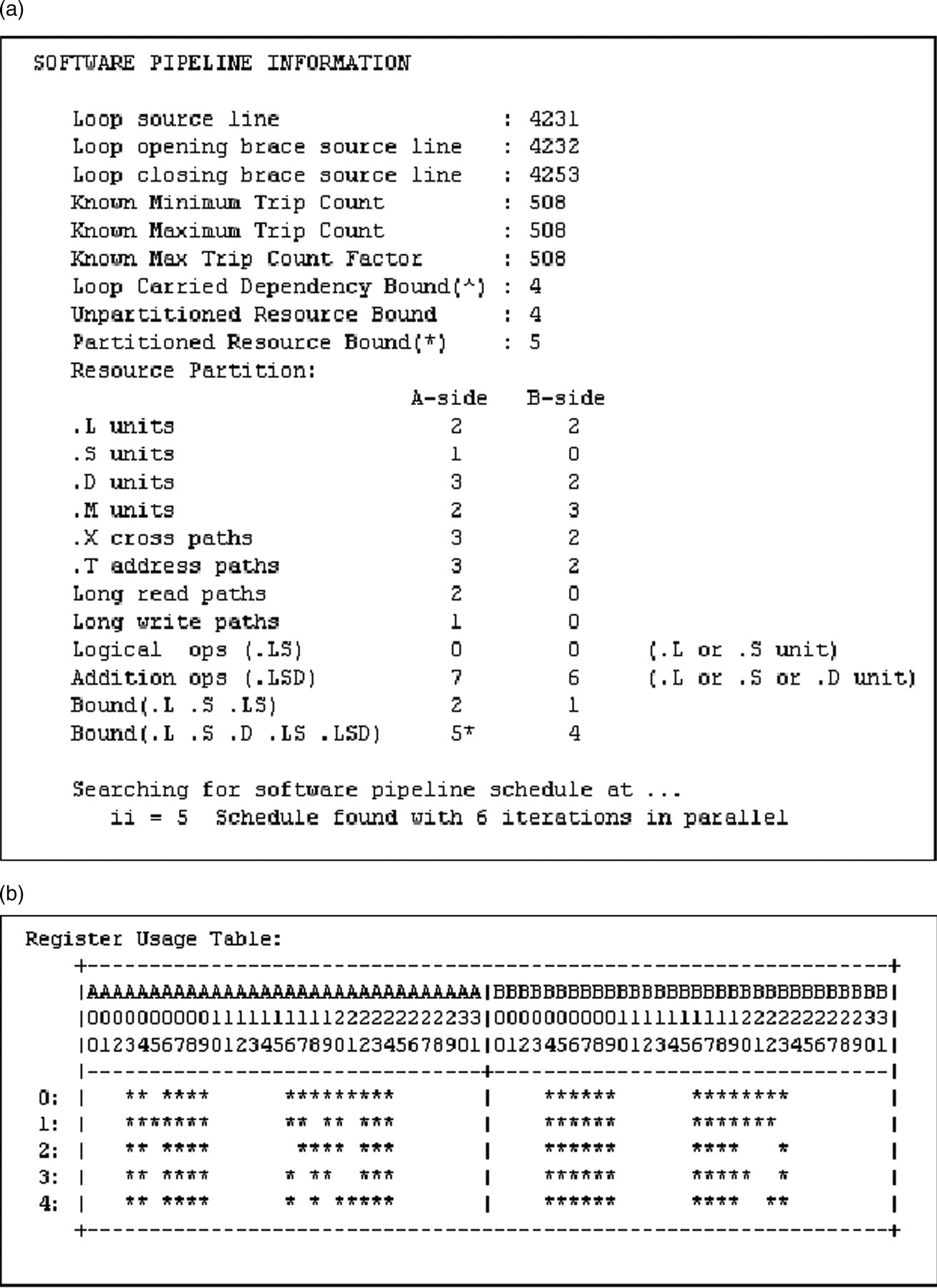
Parallelism information: (a) resource partition, (b) register usage

Figure 9
Comparison with MATLAB I: (a) MATLAB output image, (b) DSP output image. DSP, digital signal processor

Figure 10
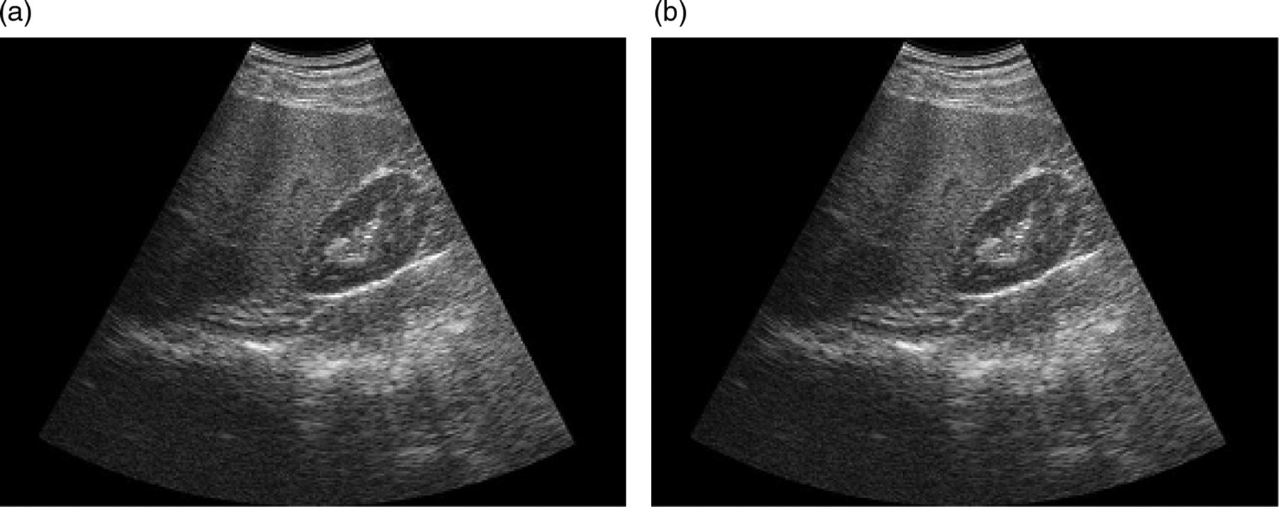
Comparison with MATLAB II: (a) MATLAB output image, (b) DSP output image. DSP, digital signal processor

Table 5
Cycle statistics for the pipelined functions

Function name Cycles

Resize 131,182

interpoleX3 499,593

interpoleX1_5 844,884

interpoleX2_4 458,645

interpoleY3 987,709

interpoleY1_5 844,524

interpoleY2_4 365,770

toCart3 1,475,564

toCart1_5 1,017,529

toCart2_4 55,862

Table 6
Comparison with MATLAB output

Image no. MSE RE UQI

Figure 9 4.56 0.1853 0.9996

Figure 10 4.88 0.1917 0.9992

MSE, mean square error; RE, relative error; UQI, universal quality index

Table 7
DSC performance comparison

Reference Interpolation Raw image size Frame rate (fps) Platform used

8 Linear 256 × 256 190 FPGA

4 Linear 512 × 512 114 FPGA

22 Linear and cubic 257 × 512 34 DSP

5 Bilinear 256 × 128 67 PC

Proposed Proposed 512 × 256 83 DSP

DSC, digital scan conversion; DSP, digital signal processor; PC, personal computer

Conclusion

A realtime digital scan converter for ultrasound sector scanners has been described in this paper. The algorithm utilizes warped distance-based adaptive bilinear interpolation with selective sampling which performs well for edge regions when compared with bilinear and bicubic interpolations. A modified selective sampling technique reduced the computational complexity. The structure of the entire DSC process is improved to meet the requirement of software pipelining. Conditions and floating point calculations are avoided to qualify the pipelining. The proposed algorithm is simulated using a TI DSP of series TMS320C64x+ cycle accurate simulator which supports parallelism and software pipelining. By interpolating data in both axial and radial directions, the image quality does not suffer even after zooming in or zooming out of the image. The proposed technique of variable sampling is applicable for raw image acquired by phased array transducers. In case of a linear array transducer coordinate conversion is not needed. Therefore, only uniform interpolation technique is enough to increase the resolution of the ultrasound image. For input raw image size 512 × 256 and VGA output the DSP simulation of the proposed algorithm supports 83 fps which is more than adequate for realtime display. The frame rate will go down with an increase in the display size.

Process	Function
Resizing	Resize	Resize the image.
Interpolation in the X-direction	interpoleX3	Interpolate the pixels on virtual scan line number 3 in all regions
	interpoleX1_5	Interpolate the pixels on virtual scanline numbers 1 and 5 in region k = 2, 3
	interpoleX2_4	Interpolate the pixels on virtual scanline numbers 2 and 4 in region k = 3
Interpolation in the Y-direction	interpoleY3	Interpolate virtual scan points on scan line 3 in all regions
	interpoleY1_5	Interpolate virtual scan points onscan lines 1 and 5 in region k = 2, 3
	interpoleY2_4	Interpolate the pixels on virtual scanpoints numbers 2 and 4 in region k = 3
From polar-to-Cartesian conversion	toCart3	Coordinate conversion of pixels on thereal scan lines and scan line 3
	toCart1_5	Coordinate conversion of pixels onscan lines 1 and 5
	toCart2_4	Coordinate conversion of pixels onscan lines 2 and 4

Interpolation algorithm	MSE	PSNR (dB)
Bilinear interpolation	39.07	15.13	32.21	36.33
Bicubic interpolation	36.53	13.15	32.50	36.93
Warped adaptive bilinear interpolation	34.97	11.91	32.69	37.36

Interpolation algorithm	FOM	EKI
Bilinear interpolation	0.9931	0.9964	0.7150	0.4564
Bicubic interpolation	0.9935	0.9978	0.8988	0.6210
Warped adaptive bilinear interpolation	0.9936	0.9979	0.8845	0.5924

Interpolation	Addition	Multiplication
Bilinear	10P + 2Q	10P + 2Q
Proposed	27P + 9Q	24P + 8Q
Cubic	50P + 10Q	80P + 16Q

Function name	Cycles
Resize	131,182
interpoleX3	499,593
interpoleX1_5	844,884
interpoleX2_4	458,645
interpoleY3	987,709
interpoleY1_5	844,524
interpoleY2_4	365,770
toCart3	1,475,564
toCart1_5	1,017,529
toCart2_4	55,862

Image no.	MSE	RE	UQI
Figure 9	4.56	0.1853	0.9996
Figure 10	4.88	0.1917	0.9992

Reference	Interpolation	Raw image size	Frame rate (fps)	Platform used
8	Linear	256 × 256	190	FPGA
4	Linear	512 × 512	114	FPGA
22	Linear and cubic	257 × 512	34	DSP
5	Bilinear	256 × 128	67	PC
Proposed	Proposed	512 × 256	83	DSP

Footnotes

ACKNOWLEDGMENT

This work has been supported by GE Medical Systems India Pvt Ltd, Bangalore, India.

DECLARATIONS

The authors have no conflicts of interest to declare.

Appendix

Mean-square error and relative error of DSP output image are defined as

where I(x,y) is the MATLAB output image, Î(x, y) is the DSP output image and M,N are the dimensions of the images.

References

Ophir

, Maklad

. Digital scan converters in diagnostic ultrasound imaging. IEEE Proceedings 1979;4:654–64

Lee

, Kim

, Park

. Analysis of a scan conversion algorithm for a real-time sector scanner. IEEE Trans Med Imaging 1986;2:96–105

Ophir

, Brinch

. Moiré undersampling artifacts in digital ultrasound. Ultrasonic Imaging 1982;4:311–20

Oppenheim

, Shafer

. Discrete-time Signal Processing. Englewood Cliffs, NJ: Prentice Hall, 1989

Ahn

D-K

, Jeong

M-K

, Kwon

S-J

, Bae

M-H

. A digital scan conversion algorithm using Fourier transform. Proceedings IEEE Ultrasonics Symposium, 2009

Wang

, Deng

, Li

, Xie

, Guo

, Zheng

. Software implementation of real-time digital scan converter. Proceedings International Conference on Biomedical Engineering and Informatics (BMEI'10), 2010, 574–7

Berkhoff

, Huisman

, Thijssen

, Jacobs

EMGP

, Homan

RJF

. Fast scan conversion algorithms for displaying ultrasound sector images. Ultrason Imaging 1994;16:87–108

Richard

, Arthur

. Real-time ultrasonic scan conversion via linear interpolation of oversampled vectors. Ultrason Imaging 1994;16:109–23

Fritsch

, Parrilla

, Martinez

, Jiménez

. A multirate scan conversion method. Ultrasonics 2000;38:179–82

10.

Chang

, Yen

, Shung

. High-speed digital scan converter for high-frequency ultrasound sector scanners. Ultrasonics 2008;48:444–52

11.

Gribbon

, Bailey

. A novel approach to real-time bilinear interpolation. IEEE International Workshop on Electronic Design, Test and Applications 2004, 126–31

12.

Keys

. Cubic convolution interpolation for digital imaging processing. IEEE Trans Acoustics, Speech Signal Proces, 1981;29:1153–60

13.

Hou

, Liu

. A filtering based scan conversion method in ultrasound system. World Congress on Medical Physics and Biomedical Engineering 2006 2007;14:1494–7

14.

Parker

, Kenyon

, Troxel

. Comparison of interpolation methods for image resampling. IEEE Trans Med Imaging 1983;1:31–9

15.

Ramponi

. Warped distance for space-variant linear image interpolation. IEEE Trans Image Proces 1999;8:629–39

16.

Hadhoud

, Dessouky

, El-Samie

FEA

. Adaptive image interpolation based on local activity levels. Proceedings of the 20th National Radio Science Conference, 2003;C4:1–8

17.

Hwang

, Lee

. Adaptive image interpolation based on local gradient features. IEEE Signal Proces Lett 2004;11:359–62

18.

Hong

, Paik

, Kim

, Lee

. An edge-preserving image interpolation system for a digital camcorder. IEEE Trans Consumer Electron 1996;42:279–84

19.

, Ma

, Shen

. Kringing interpolation based ultrasound scan conversion algorithm. IEEE International Conference on Information Acquisition, 2006, 489–93

20.

TMS320C64x/C64x+ DSP CPU and Instruction Set. Reference Guide. Texas Instruments, SPRU732H, 2008. See http://www.ti.com (last checked January 2011)

21.

TMS320C6000 Programmers Guide. Texas Instruments, SPRU198I, 2006. See http://www.ti.com (last checked January 2011)

22.

, Liu

. An embedded high performance ultrasonic signal processing subsystem. Proceedings of the International Conference on Embedded Software and Systems (ICESS ‘09), 2009, 125–30

Interpolation algorithm	MSE		PSNR (dB)
	Mandrill	Cameraman	Mandrill	Cameraman
Bilinear interpolation	39.07	15.13	32.21	36.33
Bicubic interpolation	36.53	13.15	32.50	36.93
Warped adaptive bilinear interpolation	34.97	11.91	32.69	37.36