Degrees of Return: Estimating Internal Rates of Return for College Majors Using Quantile Regression

Economic Benefits of College Education and Majors

Human capital theory posits that the labor market rewards investments individuals make in themselves (e.g., their education or training) and that these investments lead to higher salaries (Becker, 2009). Consistent with this framework, college graduates typically earn more than high school graduates. There are, however, large variations in earnings across college majors. Those who graduate with degrees in computer science, engineering, or business tend to have a significant earnings advantage—roughly 30% to 40% more—than those who major in humanities, arts, education, or history (Altonji, Arcidiacono, & Maurel, 2016; Black, Sanders, & Taylor, 2003; Ransom, 2021; Thomas & Zhang, 2005). Moreover, high-paying majors often demonstrate greater resilience during economic downturns, further contributing to the earnings disparity across majors (Altonji, Kahn, & Speer, 2016).

A human capital explanation for varying returns on college majors is that they represent distinct types of specialized human capital (i.e., skills). Research on skill-based labor scarcity argues that returns on college education depend on the relative scarcity of the acquired skills. For instance, Paglin and Rufolo (1990) found that differences in mean quantitative GRE scores positively affect earnings differentials across majors, while average verbal GRE scores do not significantly relate to earnings. This finding suggests that quantitative skills are more valuable, leading to higher expected earnings for college majors emphasizing these skills. Grogger and Eide (1995) demonstrated that the return on math ability has increased over time. Specifically, a 1-SD increase in math ability was associated with 2% higher wages in 1978, increasing to 5% higher wages in 1986 for male workers; for female workers, this was associated with 3% higher wages in 1978, increasing to 7.5% higher wages in 1986. Weinberger (1999) supported these findings, showing that college graduates in majors with more mathematical content earn significantly more. These early works provide important insights into the heterogeneity of human capital and varying returns through college majors.

Research on SBTC emphasizes the impact of radical technological shifts on labor supply-demand frameworks (Acemoglu & Autor, 2011; Katz & Murphy, 1992). Katz and Murphy (1992) found that from 1963 to 1987, a period when the percentage of the U.S. labor force with a college degree was increasing, the “college premium”—the ratio of the average earnings of college graduates to that of high school graduates—also rose significantly. The authors maintained that demographic shifts and other supply-side factors could not fully explain the surge in the college premium and concluded that the explanation must be rooted in an increased demand for skilled workers. Recent studies reveal that the advanced cognitive and technical skills demanded by computer technologies have led to a widening wage gap between skilled and unskilled workers. Goldin and Katz (2010) reported that the college wage premium increased from 35.6% in 1980 to 59.6% in 2005, even with a substantial rise in the relative supply of college-educated workers. They further contended that the observed earnings disparities between high school and college graduates since the 1980s are due primarily to technological advancements driven by the extensive use of computers. International studies conducted by Berman, Bound, and Machin (1998) and Beaudry, Green, and Sand (2014) also provide support for SBTC.

While educational attainment or credentials are commonly used as proxies for skills in the SBTC literature, workers with equal levels of formal education may have different skill levels and apply different skills in their job duties. Research on RBTC directly measures the task composition of occupations and analyzes skill requirements in the workplace (Acemoglu & Autor, 2011; Autor, Levy, & Murnane, 2003; Goos, Manning, & Salomons, 2014). The task approach offers a micro-foundation for connecting aggregate demand for skills in the labor market to specific work tasks. Acemoglu and Autor (2011) categorized occupations on the basis of cognitive versus manual tasks and routine versus nonroutine tasks: Cognitive tasks require more mental activity, whereas manual tasks require more physical activity; and routine tasks involve specific repetitive activities, whereas nonroutine tasks require flexibility, creativity, problem solving, or human interaction. They further suggested that technological advancements often automate repetitive and predictable tasks, such as data entry or basic assembly line work, leading to a decrease in the demand for workers who specialize in routine tasks.

Supporting RBTC, Goos and Manning (2007) argued that computer technology replaces workers who perform routine manual and cognitive tasks but complements workers who perform nonroutine cognitive tasks. Autor, Katz, and Kearney (2006) found an increase in the share of low- and high-paying jobs, but a decrease in the share of middle-wage jobs since the 1990 census. Autor and Handel (2013) reported that a 1-SD increase in the abstract task scale is associated with a 20% hourly wage premium, while similar increases in routine and manual tasks are associated with wage penalties of 10% and 19%, respectively. Complementary to the supply-demand-institutions framework, Deming (2023) found that the accumulation of college graduates in professional, nonroutine occupations, which provide ample opportunities for on-the-job learning, has contributed to an increase in college premiums.

Taken together, these three theoretical arguments suggest, to varying degrees, that the labor market favors college graduates over high school graduates, with certain college majors, particularly those requiring math and other high-demand skills, as well as those closely related to nonroutine tasks, commanding greater economic benefits. Recent research confirms that employers perceive college majors as skill bundles, with different majors being associated with occupations requiring distinct skill sets. Hemelt et al. (2023) analyzed a comprehensive dataset of online job ads posted in the United States between 2010 and 2018 and found that jobs requiring high levels of cognitive, financial, and project management skills offer substantially higher wages compared with those with lower demand for these skills. Notably, college majors account for the vast majority of variation in the demand for different skills. For example, college majors explain 69%, 84%, and 71% of the variation in the demand for cognitive, financial, and project management skills, respectively. Stinebrickner, Stinebrickner, and Sullivan (2018) found in their longitudinal task-based skills dataset that business majors spend more than 33% more time skilled tasks involving information interaction than humanities majors. These results highlight the significance of college majors as key indicators of skills in the labor market, establishing an important nexus between college majors and skills.

Consistent with these theories, a growing body of literature has demonstrated the existence of significant variation in economic returns across college majors. Berger (1988) analyzed the present value of expected lifetime earnings of five major categories, and found that during the 1970s, earnings profiles for liberal arts and education majors plateaued, suggesting a growing advantage for science and engineering majors. Grogger and Eide (1995) found increases in the premiums for fast growing majors, suggesting that the exogenous demand for skills associated with these majors must have increased at an even faster rate. The widely observed increase in the wage premium for college degrees during the 1980s resulted partly from changes in college graduates’ skill levels due to shifts in distribution from less technical (e.g., education) to more technical majors (e.g., science, technology, engineering, and mathematics [STEM], business). Examining the historical relationship between education and technology, Goldin and Katz (2010) argued that merely holding a college degree no longer guarantees high earnings; instead, focusing on specific fields and acquiring advanced skills in targeted areas can yield higher returns. In an updated analysis, Autor, Goldin, and Katz (2020) further suggested that the primary source of the observed growth in wage inequality has occurred within the same educational level rather than between educational levels. Specifically, the largest portion of the increased wage disparity since 2000 is attributed to escalating inequality among college graduates, while wage inequality relative to non-college-educated workers has changed very little.

Economic Costs of College Education and Majors

Attending college entails both benefits and costs. Rapid growth in college expenses in recent decades is well documented in the literature. According to the most recent data from the College Board (Ma & Pender, 2022), between academic years 1999–2000 and 2019–2020, average tuition and fees rose, on average, by 3.5% per year at public 4-year institutions and by 2.2% at private, nonprofit 4-year institutions, after adjusting for the Consumer Price Index.

Less well documented is the variation in college costs across different majors. First, the distribution of majors varies across institutions. For instance, engineering and other STEM majors are overrepresented, while humanities and arts majors are underrepresented at research and doctoral universities compared with master's and baccalaureate institutions. As such, varying costs across colleges may lead to different average costs for different college majors. Second, within the same institutions, colleges and universities may charge different tuition and fees for different majors, a practice that has become increasingly common (Cornell Higher Education Research Institute, 2012; Wolniak, George, & Nelson, 2018). Many institutions charge higher tuition for engineering and health than for other majors. This differential tuition pricing partly reflects disparities in costs associated with different majors. Altonji and Zimmerman (2018) reported that the cost of producing graduates in engineering is almost double that of producing business graduates. On the basis of departmental-level data, Hemelt et al. (2021) found that instructional costs for electrical engineering were 109% higher than those for English. Disciplines such as STEM and health exhibited costs on the higher end of this spectrum. Using the phased introduction of differential tuition policies over time, Stange (2015) observed a notable decrease in the proportion of students opting for engineering and business majors in reaction to elevated costs. Finally, students in different fields may face varying opportunities for grant aid, which could lead to differences in net costs across majors. Specifically, students in STEM fields may have better opportunities for grant aid (Evans, 2017), especially at the state and institutional levels, thereby decreasing their college costs.

Studies of IRR

Studies of IRR for college education are not new, but the vast majority have focused on college education as a whole without estimating major-specific returns (Leslie & Brinkman, 1988; Psacharopoulos & Patrinos, 2018). For example, Leslie and Brinkman (1988) conducted a meta-analysis of 43 estimates from 26 IRR studies of college education and found a mean of 12.4% with a 95% confidence interval of 11.4% to 13.4%. Psacharopoulos and Patrinos (2018) found that among high-income countries, the private return on higher education was about 12% on the basis of 54 studies conducted after 2000. It appears that although estimates from individual studies vary, the central tendency is strikingly consistent over time.

Only very limited research has been conducted on IRR across college majors. Koch (1972) used cost data from Illinois State University for 1968 to 1969 and found that mathematics and economics were associated with the highest IRRs, while education, fine arts, and history were found to have the lowest IRRs. More recently, Lobo and Burke-Smalley (2018) used aggregate data on lifecycle earnings from the Hamilton Project at the Brookings Institution to estimate net present value and IRRs for various majors in the United States. The results indicate that certain majors such as education are associated with negative net present values when students take more than 4 years to graduate. It is worth noting that the data from the Hamilton Project are based on ACS data from 2009 to 2012. Our study extends Lobo and Burke-Smalley’s work by leveraging individual-level ACS data from 2009 to 2021. This time frame is significant, as it coincided with economic growth and a tightening labor market in the aftermath of the 2008 Great Recession. Recent research indicates a stagnation or even decline in college wage premiums after the Great Recession (Bengali et al., 2023). Similarly, Ashworth and Ransom (2019) found that the increasing college wage premium for the 1950–1970 birth cohort was followed by a flattening for the 1980–1984 birth cohort. Given these findings, it becomes crucial to examine whether the IRR on college education has decreased during this specific period of time.

More important, the individual-level data in the ACS, when combined with the detailed financial data from the National Postsecondary Student Aid Study: 18 Administrative Collection (NPSAS: 18 AC), enable us to investigate heterogeneity in IRRs by sex and race/ethnicity groups, as well as across the earnings distribution. Research on the earnings gap has revealed that, conditional on the same major, women tend to gravitate toward occupations with potentially lower wages, fewer hours, and less demanding tasks compared with men (Sloane, Hurst, & Black, 2021; Stinebrickner et al., 2018). However, the return to college education is based on a comparison between high school and college graduates within the same sex group. Notably, many studies have demonstrated that a college education exerts a larger impact on earnings for women than for men. For instance, Dougherty (2005) suggested that in addition to enhancing skills and productivity for both men and women, education also influences factors such as discrimination, preferences, and circumstances for women. On the cost side, women may encounter lower opportunity costs when attending college. Therefore, we anticipate that women experience a higher IRR compared with men.

Likewise, while minorities, especially Black and Hispanic individuals, tend to earn less than their White counterparts with equivalent educational attainment, the earnings differentials between high school and college graduates are quite consistent across race/ethnicity groups among women. For men, the earnings increase is slightly more pronounced for White men compared with Black and Hispanic men (Hout, 2012; Julian & Kominski, 2022). Such earnings disparities can lead to variations in IRRs across different race/ethnicity groups. For instance, Cooper and Cohn (1997) calculated the IRR for college education using data from the 1985 wave of the Panel Study of Income Dynamics and identified disparities in IRR between sex and racial groups. In particular, Black women had a higher IRR than both White men and women, while Black men had the lowest IRR among all four groups. On the cost side, detailed financial data from NPSAS: 18 AC show significant variations in net college costs by race/ethnicity. Specifically, Black and Hispanic students, on average, face approximately $6,000 less in net college costs than their White and Asian counterparts. These discrepancies in both earnings and college costs likely lead to varying IRRs across race/ethnicity groups.

Finally, it is possible that returns on college education as well as major choices may be different for individuals at different points of the earnings distribution. For example, the earnings advantage of some majors, such as computer science and business, may be greater for individuals who are at the upper end of the earnings distribution than for those at the lower end. This seems to be supported by the anecdotal evidence that many of the highest paying positions are in the business and information technology sectors. In contrast, although health majors, on average, have earnings on par with STEM and business, they do not have as much of an advantage at the higher echelons of the earnings spectrum. Estimating IRRs at different distributional points would yield additional information beyond the “average” return. The large sample size in the ACS (2009–2021) offers reliable estimates of the earnings differences and IRRs at different points of the distribution.

Data, Sample, and Variables

The ACS collects comprehensive demographic and financial data on individuals and households each year. Since 2005, data on approximately 3 million individuals representing roughly 1% of the U.S. population has been included in the annual public microdata file. In 2009, the ACS started collecting information on undergraduate majors for individuals with baccalaureate degrees. Among individuals with baccalaureate degrees, 11.0% reported having a second bachelor's degree. In this analysis, we used only information about individuals’ first majors. Results from a separate set of analyses, which excluded individuals with dual majors, are very similar to those reported in this article and are available upon request.

The data used for this study include 13 annual ACS files from 2009 to 2021. For each annual file, we extracted the following information: place of birth, age, sex, race/ethnicity, marital status, region of residence, highest level of education attained, school enrollment status, employment status, undergraduate major, and annual wage or salary earnings. We limited the sample to individuals who met the following criteria: (a) were born in the United States and were 18 to 65 years old, (b) held either a high school diploma or a bachelor's degree as their highest level of education (and, for college graduates, provided information on college major[s]), (c) were not currently enrolled in school, and (d) had positive earnings. Applying these criteria yielded a final sample of 5.8 million individuals: 2.9 million high school graduates and 2.9 million college graduates.

We used individuals’ wage and salary earnings as the main dependent variable. In a separate set of analyses, we used total earnings because earnings other than wages and salary, such as self-employment income, may also be related to college education and majors. ACS earnings data combine 12 reference periods that lag 6 months behind the calendar year, on average. To ensure comparability across different years of ACS data, we first adjusted the reported annual income using the income adjustment factor in each ACS file. We then adjusted the income data for inflation using the Consumer Price Index published by the Bureau of Labor Statistics, converting all income into constant 2021 dollars.

We compared individuals who had completed only high school with those who had obtained only bachelor's degrees. We focused on the returns to bachelor's degrees instead of associate degrees because of their distinct costs and benefits. We excluded individuals with less than high school diplomas or with some college experience to ensure a clean estimate for the returns to 4-year college degrees relative to high school. Finally, we excluded individuals holding advanced degrees (e.g., master's, first professional, and doctorate) because obtaining a bachelor's degree and an advanced degree are separate investment decisions with their own benefits and costs. Furthermore, individuals who pursue advanced degrees might inherently differ in various ways from those who stop at bachelor's degrees. Excluding individuals with advanced degrees would minimize the bias due to these unobserved characteristics.

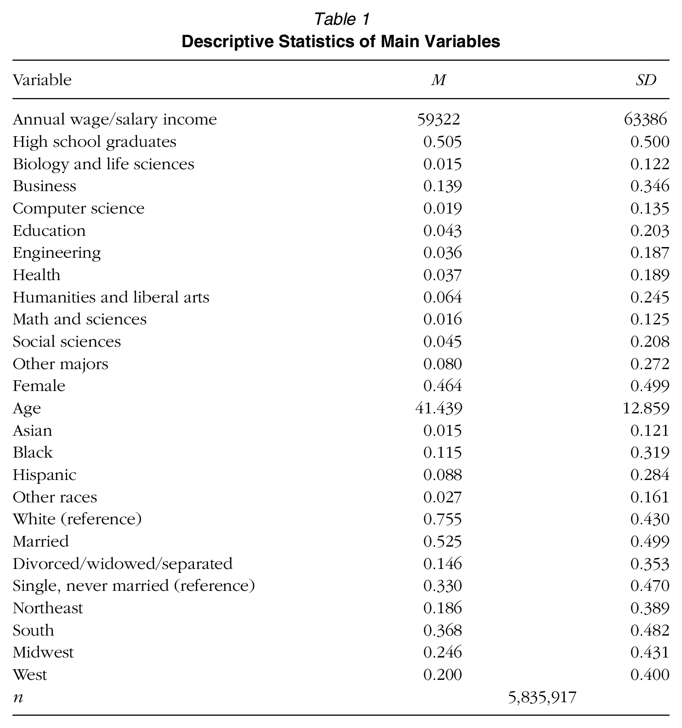
To measure college majors, we built upon work by Carnevale, Strohl, and Melton (2013) and used a crosswalk table provided by the U.S. Census Bureau to aggregate 173 detailed undergraduate fields of study in the ACS into 10 broad categories: biological and life sciences, business, computer science, education, engineering, health, humanities and liberal arts, math and sciences, social sciences, and other majors. A list of these categories and ACS majors is available in Table A1 in the Online Supplementary Materials. Individual characteristics, including age, sex, and race/ethnicity, as well as marital status (married; divorced, widowed, or separated; and single, never married), and regions (Northeast, Midwest, South, and West), were included as covariates in the analysis. These covariates were commonly used in the literature to account for individual differences. We chose not to include variables such as industry classifications or classes of workers, as these factors depend partly on college majors. Table 1 shows the list of variables used in this analysis.

OPEN IN VIEWER

Table 1

Descriptive Statistics of Main Variables

Variable	M	SD
Annual wage/salary income	59322	63386
High school graduates	0.505	0.500
Biology and life sciences	0.015	0.122
Business	0.139	0.346
Computer science	0.019	0.135
Education	0.043	0.203
Engineering	0.036	0.187
Health	0.037	0.189
Humanities and liberal arts	0.064	0.245
Math and sciences	0.016	0.125
Social sciences	0.045	0.208
Other majors	0.080	0.272
Female	0.464	0.499
Age	41.439	12.859
Asian	0.015	0.121
Black	0.115	0.319
Hispanic	0.088	0.284
Other races	0.027	0.161
White (reference)	0.755	0.430
Married	0.525	0.499
Divorced/widowed/separated	0.146	0.353
Single, never married (reference)	0.330	0.470
Northeast	0.186	0.389
South	0.368	0.482
Midwest	0.246	0.431
West	0.200	0.400
n	5,835,917

Estimating Benefits: Methods

We estimated the differences in age-earnings profiles between high school graduates and college graduates in different majors on the basis of the four-step procedure outlined by Cohn and Huches (1994) and Cooper and Cohn (1997). First, we estimated earnings equations for high school graduates and each college major. Second, because individual characteristics may differ across groups, we substituted the average characteristics of all college graduates into each earnings equation to obtain the estimated earnings for each group. Third, we predicted earnings for each age in each group on the basis of age-earnings profiles, and calculated differences between groups in predicted earnings. Finally, we used these earnings differences and estimated costs to estimate IRRs.

Mathematically, we began with the following log-linear earnings equation:

ln ( Y i ) = α 0 + β 1 age i + β 2 age i 2 + ∑ j = 1 10 γ j M j + Z i ' ξ + μ i ,

(1)

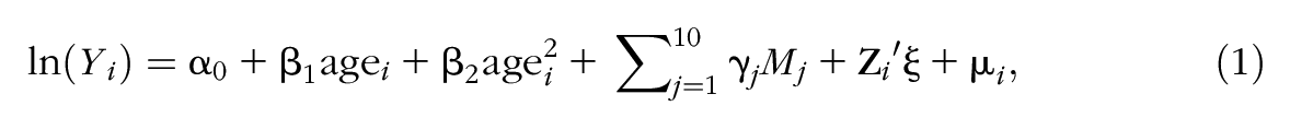
where Y_i represents individual i’s annual wage or salary earnings, and M_j represents individual i’s college major j, with high school graduates as the reference category. Z _i includes a set of covariates for individual i.

Equation 1 assumes an additive relationship between age and major, implying that the age-earnings profiles are parallel across different majors. However, this assumption may not hold, as descriptive data analyses show that different college majors tend to have different earnings trajectories over time. Therefore, we relaxed this assumption and estimated an age-earnings equation for each major group, as well as the reference group of high school graduates:

ln ( Y i m ) = α 0 m + β 1 m age i + β 2 m age i 2 + Z i ' ξ + μ im for m = 0 , 1 , … , 10 ,

(2)

where m = 0 represents high school graduates, and m = 1, . . ., 10 represents each of the 10 college majors examined in this analysis.

Furthermore, individual characteristics Z _i may differ systematically between high school graduates and college graduates, among college majors, and across age groups within college majors. For example, marital status and racial composition may differ between older and younger age groups. To account for these differences, we used the mean values of all variables (excluding age and age squared) for college graduates in the pooled sample to substitute for the Z _i values in all estimated equations:

ln ( E m ) = α ^ 0 m + Z ¯ ' ξ ^ for m = 0 , 1 , … , 10 .

(3)

Substituting ln(E_m) into Equation 2, we get

ln ( Y i m ) = ln ( E m ) + β 1 m age i + β 2 m age i 2 for m = 0 , 1 , … , 10 .

(4)

We computed earnings differences on the basis of Equation 4 for each age value from 18 to 65 years. These differences by age were then used to estimate the IRRs of different college majors relative to high school graduates using the following equation:

∑ t = 18 65 ( Y c t − Y h t ) ( 1 + r ) t − 18 − ∑ t = 18 21 C c t ( 1 + r ) t − 18 = 0 ,

(5)

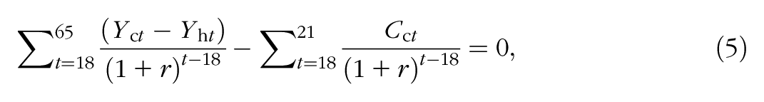
where Y_ct represents college graduates’ earnings at age t; Y_ht represents high school graduates’ earnings at age t; C_ct represents college costs for college students at age t; and r is the IRR to be estimated. In Equation 5, college costs (C_ct) are assumed to occur only during college years. It is worth noting that college students may earn income through student employment while attending college.

Equation 2 is usually estimated using the ordinary least squares method, which calculates the earnings differences at the mean of the income distribution, i.e., it determines the average differences in earnings between college graduates in different majors and high school graduates. To examine the earnings differences between college majors and high school graduates at different points of the earnings distribution, we used the quantile regression technique (Koenker & Bassett, 1978). Quantile regression aims at minimizing the following loss function:

min β ∈ R K ∑ y i > x i β θ | y i − x i β | + ∑ y i < x i β ( 1 − θ ) | y i − x i β | ,

(6)

where y_i is the dependent variable, x _i is a vector of independent variables, β is a vector of coefficients, and θ is an arbitrary distributional point to be estimated (e.g., 10th percentile, median, 75th percentile).

In addition to the advantage of estimating the earnings differences at any point of the distribution, the quantile regression method is less sensitive to outliers than ordinary least squares methods. In the case of earnings, which is likely to be positively skewed, the mean can be influenced by outliers. By contrast, the median is robust to outliers and provides a more stable representation of the earnings distribution. Empirical work using quantile regressions can be traced back to Koenker and Bassett (1978), who used the method to obtain a robust estimation when the standard normality assumption fails. In the economics of education, this technique has been applied to study changes in wage distribution (Machado & Mata, 2005), the link between education and wage inequality (Lemieux, 2006), and intergenerational earnings transfer (Eide & Showalter, 1999). Quantile regression has also been used to study education quality. For example, results based on quantile regression suggest that graduating from high-quality colleges, especially private elite institutions, would both lift and stretch the earnings distribution (Zhang, 2005).

In this study, we used quantile regression to estimate Equation 2 at deciles of the earnings distribution. The results from these regressions are used to estimate the IRRs for each decile. In other words, we compare the earnings of different college majors to the earnings of high school graduates at equivalent distributional positions. This comparison is based on the assumption that an individual's earnings rank remains unchanged between the observed and counterfactual scenarios. Simply put, those who earn well as college graduates would also be strong earners without college degrees, and the same goes for those at the lower end of the earning spectrum. This concept, known as “rank invariance,” is the identifying assumption of the quantile regression approach (Chernozhukov & Hansen, 2006; Koenker, 2017). However, in observational studies like ours, the key policy variables (e.g., college education and majors) are likely endogenous, leading to bias in the estimated effects. For instance, a college graduate positioned at the median earnings level among peers of college graduates might earn more than the median high school graduate, even without a college education.

To make the assumption of “rank invariance” more tenable, it is essential to determine how much of the observed difference between college and high school graduates can be attributed to college education rather than to observed and unobserved characteristics. Because of the absence of comprehensive ability measures and other characteristics in the ACS, we relied on estimates from the existing literature to adjust for this selection bias. Ashworth et al. (2021) developed a dynamic model to account for unobserved heterogeneity. Their analysis, based on the National Longitudinal Survey of Youth 1997 cohort, indicated that about 37% of the raw gap between high school and college graduates can be attributed to individual heterogeneity. ² Our calculations, derived from Equation 2, have already adjusted for some covariates such as sex, race/ethnicity, marital status, and regional differences, which account for about 11% of the observed difference. Subtracting that from Ashworth et al.’s 37% leaves about 25%, which is in line with other studies exploring the returns on college education using ACS data, as seen in works by Lobo and Burke-Smalley (2018) and Webber (2014). To illustrate the influence of selection bias on the estimation of IRRs, we undertook three separate analyses in the initial step, adjusting for 0%, 25%, and 50% selection, respectively. We applied 25% as our preferred selection adjustment in main analyses.

We applied the same selection adjustment when estimating opportunity costs for college students. Besides the earnings college students make while studying, they also face opportunity costs. In Equation 5, these costs are proxied by the earnings of high school graduates aged 18 and 21 years. However, if we assume that college students would have earned more than their high school counterparts had they not attended college, an adjustment is necessary. To do this, we used log-earnings equations to estimate the earnings difference between young workers (aged 22–25 years) who are high school and college graduates, yielding an estimate of 0.472, or 60%. We then assumed that 25% of the gap (15% in absolute terms) could be attributed to selection. This 15% earnings advantage was then incorporated into our calculation of opportunity costs for college students. In other words, we used a consistent selection adjustment when assessing both the opportunity costs borne by college students and the earnings differential between high school and college graduates.

Estimating Costs: Data and Assumptions

Estimating costs is a critical step of IRR analysis. IRR is highly sensitive to costs, which are incurred during the college years, whereas the benefits from college education are accrued over a much longer period of time. Moreover, the present value calculation for IRR gives greater weight to costs in the near term compared with benefits in the future. As Leslie and Brinkman (1988) suggested, it is not a stretch to view IRR studies as cost studies rather than studies of returns. When calculating the direct and opportunity costs of attending college, we made two assumptions. First, we assumed individuals attended college full-time for 4 years between the ages of 18 and 21 years. Despite varying college pathways and attendance patterns (e.g., later start or part-time attendance), this assumption is reasonable, as part-time attendance may result in similar overall costs because of reduced annual expenses and extended duration. Second, we used estimated average costs of college education for specific student groups to calculate IRRs, instead of using the actual costs for each individual. This was necessary because the costs of college education vary significantly across individuals attending different colleges and universities. Although individual-level financial data in the NPSAS enabled us to estimate average costs at each institution, these data cannot be merged with ACS data, which do not identify specific colleges where individuals obtained their degrees. Nonetheless, we were able to estimate the average costs by race/ethnicity across different college majors, as both NPSAS and ACS contain these data elements.

To estimate the direct costs of college education, we used detailed financial data from NPSAS: 18 AC, a national study of undergraduate and graduate students enrolled in Title IV institutions between July 1, 2017, and June 30, 2018. The NPSAS: 18 AC undergraduate file contains data collected from approximately 1,870 institutions: 1,160 public, 480 private nonprofit, and 230 for-profit institutions. The data collection includes roughly 5,000 undergraduates from each state, totaling about a quarter million undergraduates in the final sample. The large number of institutions and students provides a reliable data source for assessing college-related costs and financial aid for college students. It is important to note that the college costs in this study are derived from NPSAS: 18 AC and have been adjusted to 2021 real dollars. As a result, the IRRs estimated here most accurately represent students who attended college in recent years, under the assumption that their future earnings align with recent trends when adjusted for inflation. Thus, the IRRs from our study are real rates of return. The nominal IRRs before adjusting for inflation are typically 2% to 3% higher than these real rates.

We focused on full-time college students who attended 4-year institutions to calculate the total costs for this group, which included costs such as tuition and fees, books and supplies, room and board, transportation, and other education-related personal expenses. One point of contention is whether nontuition expenses, such as room and board, books and supplies, and transportation, should be included in the calculation of IRRs. Nontuition costs can be substantial. Financial data in NPSAS: 18 AC indicate that the average cost of tuition and fees for full-time attendance at 4-year institutions is slightly over $20,000, with an additional $15,000 for nontuition expenses. Among nontuition costs, books and supplies are directly linked to college education. Unfortunately, NPSAS does not itemize nontuition costs. For books and supplies, a recent national survey by the National Association of College Stores (2023) indicates a downward trend in spending on course materials, which stood at $281 for the 2022–2023 academic year. At the same time, students spent roughly $700 on technology. Hence, we incorporated $1,000 for books and supplies into our estimate of college costs.

Other nontuition expenses, especially room and board, are costs individuals would incur even if they were not attending college. Nevertheless, the expenses associated with food and housing can be significantly higher, especially for those relocating to attend college. Therefore, we argue that a portion of these nontuition costs should be included. In our analysis, we undertook three scenarios, factoring in 0%, 50%, and 100% of nontuition costs (excluding books and supplies) as attributable to college education.

To estimate the specific IRRs for race/ethnicity groups across college majors, we calculated the average costs for each group and adjusted these values to 2021 constant dollars for comparison with income data in the ACS. Table 2 reports a detailed breakdown of the average costs by race/ethnicity across college majors. We did not provide a cost breakdown by sex, because of the small sample sizes for female students in certain majors such as mathematics, which made it difficult to provide reliable estimates. Additionally, costs are generally consistent between the two groups for majors where both men and women are well represented. Table 2 shows significant differences in college costs across racial groups. Specifically, Black and Hispanic students had the lowest overall costs because of low costs of attendance and high grant aid.

OPEN IN VIEWER

Table 2

Average College Costs Across Majors, by Race/Ethnicity, National Postsecondary Student Aid Study, 2018

	College	Biology	Business	Computer Science	Education	Engineering	Health	Humanities	Mathematics	Social Sciences	Other
All	27,200	26,549	28,333	27,116	22,686	27,998	25,590	28,987	27,165	28,025	26,601
Asian	29,605	28,452	30,988	29,831	19,962	30,460	26,085	31,822	38,020	30,332	28,463
Black	23,000	22,598	22,894	22,656	20,114	26,299	23,889	23,396	22,694	23,785	22,321
Hispanic	22,020	21,284	24,939	24,245	19,873	19,428	22,736	23,312	17,657	20,648	23,019
White	28,888	28,203	29,666	27,762	23,500	30,316	26,336	30,859	28,675	31,408	28,676
Other	27,469	28,709	26,468	26,943	23,312	29,745	26,635	30,664	27,572	27,018	25,071

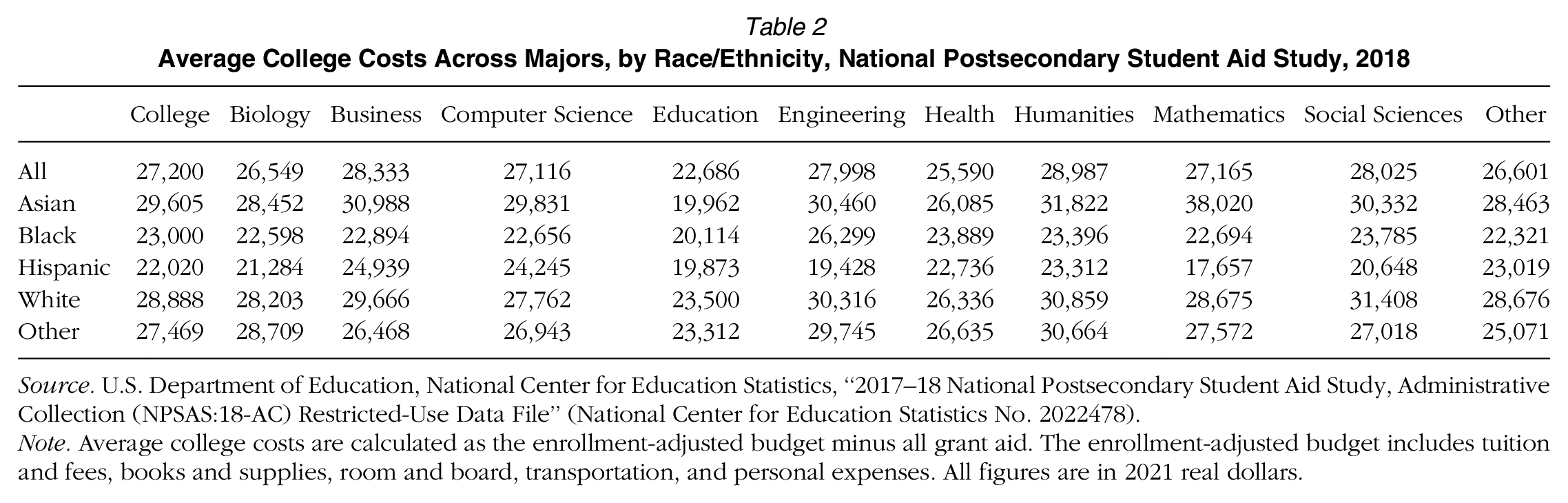
Source. U.S. Department of Education, National Center for Education Statistics, “2017–18 National Postsecondary Student Aid Study, Administrative Collection (NPSAS:18-AC) Restricted-Use Data File” (National Center for Education Statistics No. 2022478).

Note. Average college costs are calculated as the enrollment-adjusted budget minus all grant aid. The enrollment-adjusted budget includes tuition and fees, books and supplies, room and board, transportation, and personal expenses. All figures are in 2021 real dollars.

Students often receive a substantial amount of grant aid to offset college expenses. NPSAS: 18 AC reveals that students received an average grant aid of just over $10,000 from various sources: $2,250 from federal, $1,580 from state, $6,780 from institutional, and $340 from private sources. We deducted these grant aids from the budgeted costs to determine the net cost of attending college. We did not deduct other financial aid (e.g., loans) from these costs. Moreover, many college students work while in college. Recent data from the National Center for Education Statistics show that about 40% of full-time students at 4-year institutions have jobs (De Brey et al., 2023). Considering the widespread undergraduate employment, it is necessary to factor in the income students earn while in college. We used NPSAS 12 to estimate the yearly income of full-time students between the ages of 18 and 21 years who were attending 4-year colleges and obtained an average income of $2,740 per year, or $3,268 in 2021 constant dollars. ³

Earnings Equations: Median Regression

Figure 1 presents the age-earnings profiles across different college majors using locally weighted regression. As outlined in the “Data and Methods” section, the age range for high school graduates was set between 18 and 65 years, while the age range for college graduates was set between 22 and 65 years. The graphs indicate a few noteworthy observations. First, the age-earnings profiles exhibit the expected concave shape, with earnings increasing early in careers and decreasing in later years. This pattern is observed for both male and female college graduates, as well as for high school graduates and each college major. Second, age-earnings profiles differ by major, with distinct starting points, growth rates, and maximum earnings. For instance, among male college graduates, Engineering majors have much higher starting salaries and a steeper growth trajectory in their early careers compared with others. Health majors display a relatively flat earnings profile in later years, in contrast with other majors that experience significant declines. These observations highlight the importance of estimating separate earnings equations for each major. Third, while male and female college graduates have comparable starting salaries, men experience faster earnings growth in the early stages of their careers. However, this does not necessarily translate to higher IRRs for men, as among high school graduates, men earn substantially more than women as well.

OPEN IN VIEWER

Figure 1

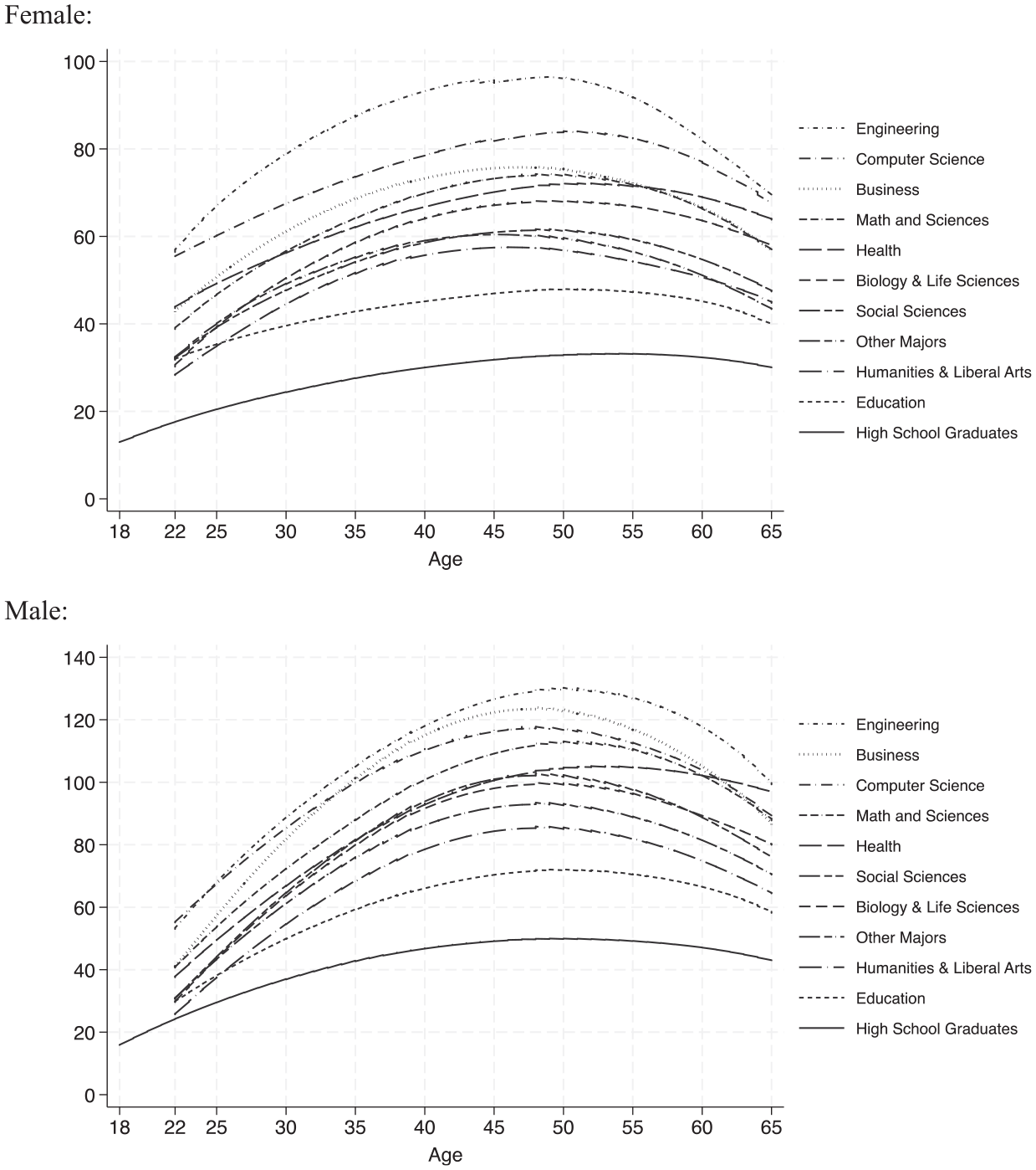
Annual earnings (in $1,000) and age using locally weighted regression.

While Figure 1 provides an overview of the average age-earnings profiles across different college majors, there are significant variations in the earnings gap between high school and college graduates and across different college majors depending on an individual's position in the earnings distribution. For some majors such as engineering, computer science, and business, earnings advantages over high school graduates and other majors increase as individuals move up the earnings distribution, suggesting that graduates of these majors not only earn higher average salaries but also tend to have a much better chance of reaching the top of the earnings distribution. For example, among men aged 45 to 50, the earnings ratio of business majors to high school graduates is 2.16 at the 10th percentile and increases to 2.62 at the 90th percentile of their respective distributions. Conversely, earnings advantages for majors such as education have declined higher up the earning distribution. For example, among men aged 45 to 50, the earnings ratio of education majors to high school graduates stands at 1.74 at the 10th percentile and decreases to 1.31 at the 90th percentile of their respective distributions. Figure A2 in the Online Supplementary Materials shows percentile-based earnings curves for college majors and high school graduates. These observations suggest the importance of estimating earnings gaps across different points of the distribution.

Consequently, we estimated Equation 2 separately for high school and college graduates, as well as for each college major, focusing on the deciles of the earnings distribution. We report the results of the median regression (5th decile) for women in Table A2 and for men in Table A3 in the Online Supplementary Materials; additional results for other deciles are available upon request. As expected, the results indicate a concave age-earnings profile; however, both the initial slopes and the curvatures vary across different groups. Furthermore, the results reveal significant gaps among different racial groups, with Asian and White groups generally earning more than Black, Hispanic, and other racial groups; however, there are notable differences on the basis of sex and college attainment. Among women, Asians have the highest earnings, followed by White and Hispanic women, with Black women having the lowest earnings. For men without college degrees, White men earn the most; however, for men with college degrees, Asian men lead in earnings. Marital status also is a significant factor, with married individuals earning more than those who are widowed, divorced, separated, or single. Finally, our results indicate significant differences across geographic regions, with higher earnings in the Northeast and the West than in the South and Midwest.

IRRs for College Education and College Majors

Table 3 reports the IRR for college education on the basis of median regression. In the far left column, in which only tuition and book costs are considered and without any selection adjustment, the IRR is 16.88% for women and 14.48% for men. Meanwhile, in the far right column that incorporates all tuition and nontuition expenses with a 50% selection assumption, the IRR is 5.08% for women and 4.96% for men. On the basis of our earlier discussions, our preferred assumptions are represented in the central column. This model incorporates tuition and fees, books and supplies, 50% of other nontuition costs, and a 0.25 selection adjustment. These assumptions are used in all subsequent tables.

OPEN IN VIEWER

Table 3

Internal Rates of Return for College Majors (Percentages) Evaluated at the Median on the Basis of Different Assumptions of Costs and Selection Adjustments

	Tuition and Books only			Tuition, Books, 50% Nontuition			Tuition, Books, Nontuition
	0	0.25	0.50	0	0.25	0.50	0	0.25	0.50
Female	16.88	12.15	7.74	13.59	9.88	6.21	11.41	8.30	5.08
Male	14.48	10.47	6.71	12.40	9.06	5.74	10.88	7.96	4.96
Asian female	17.73	13.12	8.68	14.78	11.04	7.23	12.73	9.52	6.12
Asian male	18.71	13.66	8.95	15.74	11.63	7.57	13.65	10.12	6.51
Black female	18.33	13.13	8.48	14.02	10.26	6.58	11.44	8.41	5.27
Black male	17.13	12.13	7.68	13.50	9.74	6.10	11.20	8.11	4.96
Hispanic female	18.25	13.01	8.38	14.05	10.25	6.57	11.53	8.45	5.29
Hispanic male	15.95	11.42	7.35	13.02	9.49	6.06	11.07	8.11	5.08
White female	16.22	11.69	7.41	13.25	9.62	5.99	11.21	8.13	4.93
White male	13.60	9.87	6.31	11.83	8.65	5.45	10.49	7.68	4.75
Other female	16.63	12.00	7.62	13.34	9.70	6.05	11.16	8.10	4.90
Other male	15.74	11.37	7.28	13.21	9.64	6.11	11.43	8.35	5.18

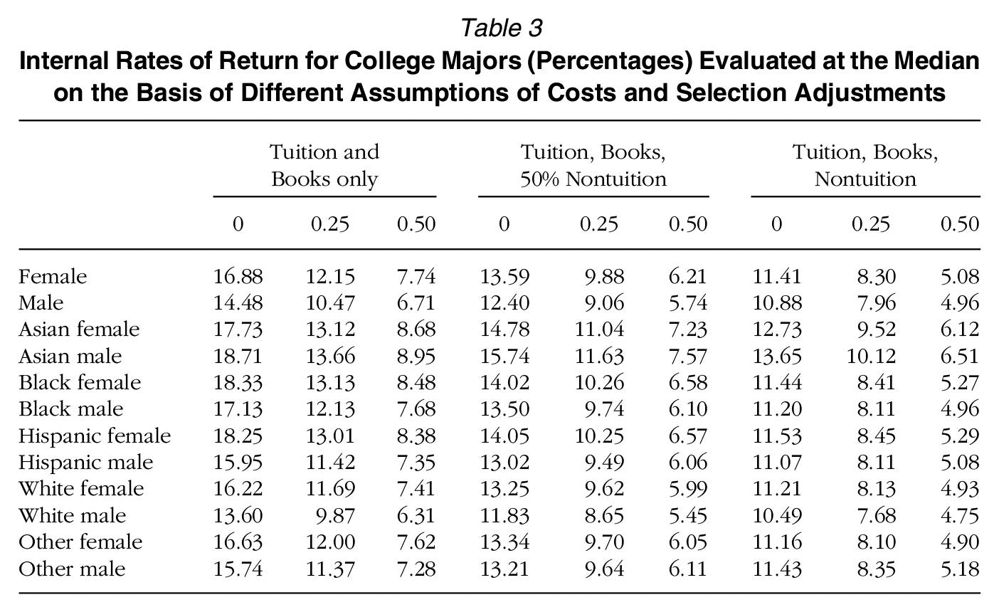
Table 4 reports IRRs for college majors across sex and race/ethnicity groups, assuming 50% of nontuition costs and a 0.25 selection adjustment. First, the IRR for a college education is estimated to be 9.88% for women and 9.06% for men. It is worth noting that our estimates are based on median earnings differences between high school and college graduates. The IRRs on the basis of mean earnings differences (see Table A4 in the Online Supplementary Materials) are 9.76% for women and 9.84% for men. In another robustness check, we used the total earnings instead of wage/salary earnings as the dependent variables (see Table A5 in the Online Supplementary Materials for detailed estimates). Results show IRRs of 9.93% for women and 9.15% for men. Second, there are large variations in IRRs across college majors. Specifically, engineering and computer science majors command the highest IRRs among all majors, exceeding 13%. Additionally, a few other majors such as business, health, and math and science have higher IRRs than the overall college population, ranging from 10% to 13%. The next tier, including biology, social science, and other majors, have IRRs of 8% to 9%. Finally, education and humanities and arts majors have the lowest IRRs, especially for men in those fields.

OPEN IN VIEWER

Table 4

Internal Rates of Return for College Majors (Percentage) Evaluated at the Median

	College	Biology	Business	Computer Science	Education	Engineering	Health	Humanities	Mathematics	Social Sciences	Other
Female	9.88	9.56	11.91	14.76	8.56	18.87	13.72	7.22	11.03	8.02	9.12
Male	9.06	7.14	10.37	12.81	3.92	13.99	8.84	4.43	9.28	6.85	7.09
Asian female	11.04	10.49	12.38	18.36	8.41	17.92	13.91	8.20	10.07	9.39	9.81
Asian male	11.63	9.23	11.82	16.61	7.39	16.19	12.84	6.52	10.47	8.27	8.35
Black female	10.26	11.00	11.00	12.91	10.41	16.13	13.26	8.11	11.13	9.05	9.06
Black male	9.74	9.21	10.85	13.06	8.69	14.65	9.30	6.41	9.65	7.78	8.49
Hispanic female	10.25	9.91	11.37	13.56	9.40	21.01	13.22	7.85	12.77	9.39	9.32
Hispanic male	9.49	8.76	10.27	12.26	6.21	16.19	9.60	5.40	11.28	8.04	7.97
White female	9.62	9.30	11.93	15.09	8.22	18.42	13.68	6.91	10.91	7.37	8.87
White male	8.65	6.67	10.06	12.43	3.25	13.26	8.45	4.00	8.89	6.26	6.63
Other female	9.70	9.15	12.68	15.19	8.93	17.65	13.73	6.92	9.91	8.26	9.31
Other male	9.64	8.04	11.37	15.98	5.40	15.05	8.33	4.13	10.50	8.13	8.10

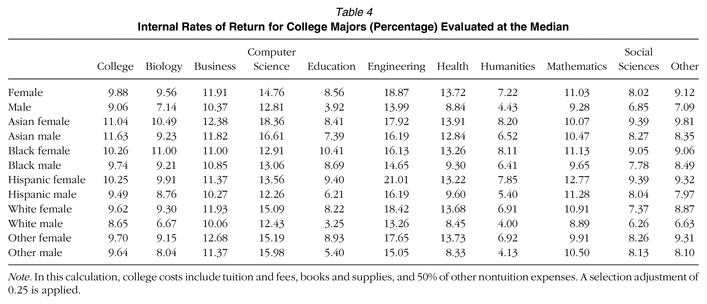
Note. In this calculation, college costs include tuition and fees, books and supplies, and 50% of other nontuition expenses. A selection adjustment of 0.25 is applied.

Third, on average, women tend to have higher IRRs than men for college education in general. However, this does not necessarily mean that female graduates earn more than their male counterparts who are men. In fact, the opposite is true: Women in our final sample earned approximately 28% less than men among college graduates and about 33% less than men among high school graduates. The lower earnings for women among high school graduates also means that women generally have lower opportunity costs while attending college. It is important to note that the differences in IRR between women and men in specific majors are usually greater than the difference in the overall college sample because women are often better represented in majors with lower IRRs.

Finally, variations in IRRs also exist across racial groups. In general, racial minority groups tend to have slightly higher IRRs than the White. The IRRs for Black and Hispanic groups are about 1 percentage point higher than that for the White group, which is due mainly to lower costs for the Black and Hispanic groups (see Table 2). In a separate simulation, when the college costs for Black and Hispanic groups were assumed to match those of the White group, their IRRs would be very similar. The Asian group has the highest IRR among all racial groups; this is due not to lower costs but primarily to their greater representation in high-paying majors such as engineering and computer science compared with other racial groups.

IRRs Across the Earnings Distribution

To estimate the IRRs at other points of the earnings distribution besides the median, we conducted quantile regressions at deciles of the earnings distribution. As illustrated in Figure 2, obtaining a college degree, especially in high-paying majors, would not only raise the entire earnings distribution but also extend its upper tail. In other words, earning a college degree has a larger effect on earnings at the top of the distribution than at the bottom. The results of the quantile regressions confirm this (see Table A6 in the Online Supplementary Materials for detailed estimates). We then used regression results to calculate the IRRs at these deciles. Figure 2 shows the IRRs associated with a college education across different points in the earnings distribution for both male and female college graduates. As one moves toward the upper end of the earnings distribution, the IRRs follow an upward trend for both samples. At the first, fifth, and ninth deciles, the IRRs are 7.66%, 9.06%, and 10.90%, respectively, for men, and 5.22%, 9.88%, and 11.32%, respectively, for women. Although the IRRs for women are generally higher than those for men, there is an exception at the first decile. One possible explanation for the lower IRR for women at the lower end of the earnings distribution is that a significant proportion of women worked less than full-time (i.e., 35 hours per week). In our final sample, more than 22% of women worked less than 35 hours per week, while the proportion for men was significantly lower at about 10%.

OPEN IN VIEWER

Figure 2.

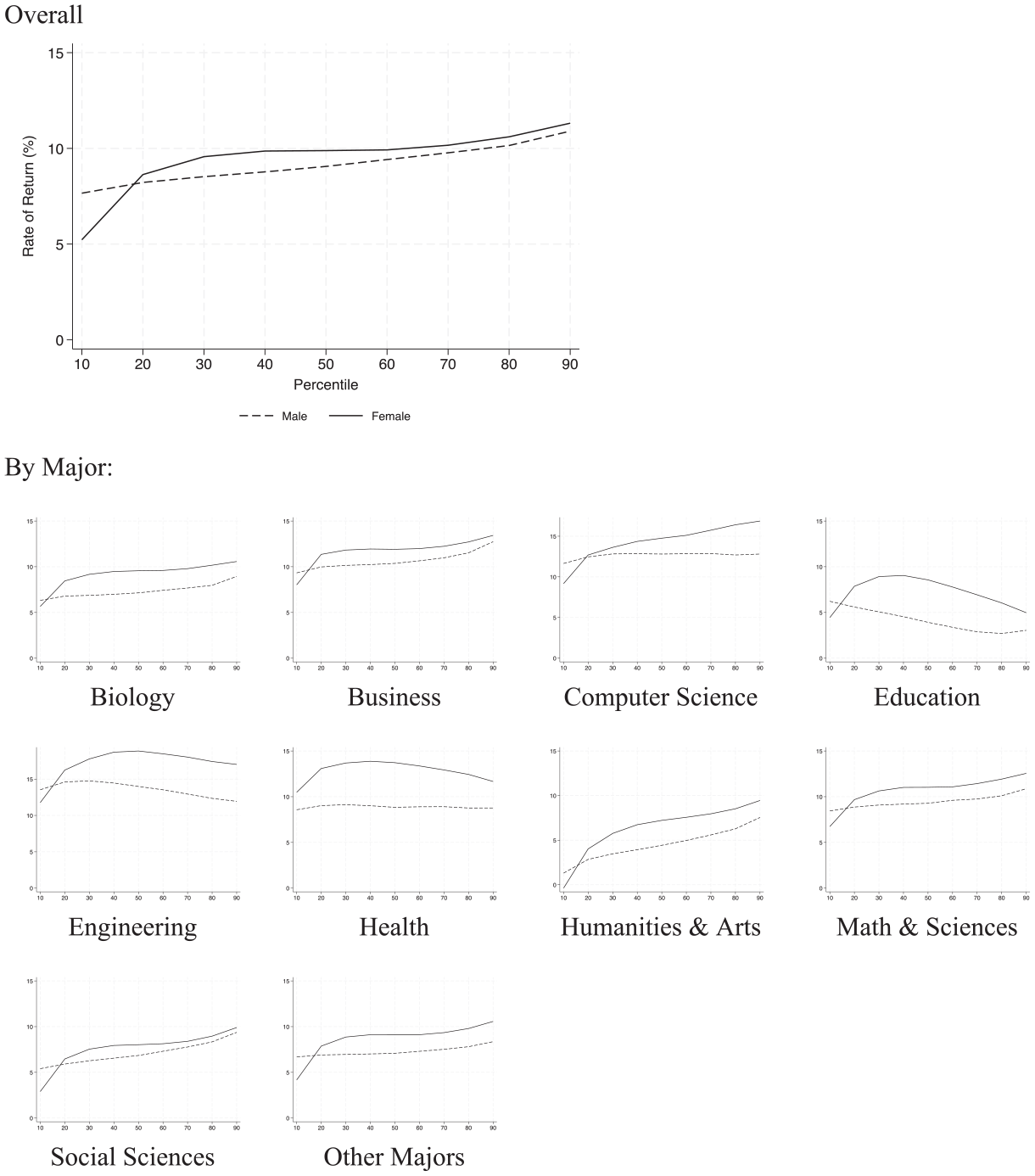
Internal rate of return of college education by decile and by college major.

Figure 2 also illustrates the results for each college major separately. The graphs show that, for most majors, IRRs increase for men and women as they move toward the upper end of the earnings distribution. However, three majors are exceptions to this trend: education, engineering, and health. For men in these majors, IRRs either remain flat (in health) or decrease (in education and engineering) as they move toward the upper end of the earnings distribution. For women in these majors, there is an initial increase in IRR up to the middle of the distribution but then a decrease as they approach the upper end of the earnings distribution. These findings suggest that graduates with degrees in these majors can expect more stable earnings but difficult for them to reach the very top of the earnings distribution compared with other majors. Recall that we estimate these IRRs by comparing the earnings differences between college and high school graduates at the same percentiles. This decline in IRRs suggests that the top earners among these college majors are not seeing their earnings rise as fast as those of their high school counterparts. These three majors also have the lowest coefficient of variation in their average earnings, corroborating the conclusion that these majors offer steady earnings advantages at different points along the distribution.

IRRs Over Time

In the final step of the analysis, we investigated changes in IRR from 2009 to 2021 by dividing the 13-year period into three periods: 2009 to 2012, 2013 to 2016, and 2017 to 2020. The year 2021 was excluded from the analysis because of the disruption caused by the COVID-19 pandemic. Results are reported in Table A7 in the Online Supplementary Materials. The findings reveal a slight decrease in IRR over time. In 2009–2012, 2013–2016, and 2017–2020, the IRRs were 10.12%, 10.08%, and 9.48%, respectively, for women, and 9.33%, 9.14%, and 8.83%, respectively, for men. Because we used the same college costs across these three periods of time, the actual decline could be more pronounced than these because of an increase in college costs faster than inflation.