Reporting Practice in Multilevel Modeling: A Revisit After 10 Years

Abstract

Multilevel modeling (MLM) is a statistical technique for analyzing clustered data. Despite its long history, the technique and accompanying computer programs are rapidly evolving. Given the complexity of multilevel models, it is crucial for researchers to provide complete and transparent descriptions of the data, statistical analyses, and results. Ten years have passed since the guidelines for reporting multilevel studies were initially published. This study reviewed new advancements in MLM and revisited the reporting practice in MLM in the past decade. A total of 301 articles from 19 journals representing different subdisciplines in education and psychology were included in the systematic review. The results showed improvement in some areas of the reporting practices, such as the number of models tested, centering of predictors, missing data treatment, software, and estimates of variance components. However, poor practices persist in terms of model specification, description of a missing mechanism, power analysis, assumption checking, model comparisons, and effect sizes. Updates on the guidelines for reporting multilevel studies and recommendations for future methodological research in MLM are presented.

Keywords

methodological development multilevel modeling reporting practices systematic review

Multilevel models (MLMs) are statistical models for analyzing clustered data, such as individuals nested within clusters, or repeated measures nested within individuals. MLMs are also known as hierarchical linear models (HLMs), random effects or random coefficients models, linear mixed effects models (LMMs) when an outcome is continuous, or generalized linear mixed effects models (GLMMs) that cover continuous as well as categorical and count outcomes. Despite the long history of MLMs, the technique and accompanying computer programs are rapidly evolving. Multilevel analyses have increased not only in quantity but also in the complexity of the models being applied. It is crucial for researchers to provide complete and transparent descriptions of the data, statistical analyses, and results, so that “scientific claims can be clearly understood, assessed, and evaluated by the reader” and “the work can be replicated with reasonable accuracy” (Appelbaum et al., 2018, p. 23). To date, there have been three published reviews of the reporting practice in MLM, two of which focus on LMMs (Dedrick et al., 2009; Schreiber & Griffin, 2004) and a more recent one on multilevel factor analyses (MFA; E. S. Kim et al., 2016).

Among the two LMM reviews, the more extensive one conducted by Dedrick et al. (2009) examined the reporting practice in 99 articles from 19 peer-reviewed journals in education and social sciences. Four main areas of methodological issues were examined, including (1) model development and specification, (2) data considerations, (3) estimation procedures, and (4) hypothesis testing and statistical inference. Within the four main areas, 41 specific issues were addressed and a checklist was developed to evaluate the multilevel applications.

Both LMM reviews indicated clear gaps between what was recommended in the methodological literature and what was reported in the applied multilevel analyses. Dedrick et al. (2009) found that details of the process of model development were often lacking. When multiple models were tested, protection against inflated familywise error or false discovery rate was generally not addressed. Predictor centering, random versus fixed slopes, and variance-covariance structures in the model specification were not clearly reported in many cases. In terms of data consideration, statistical power, evidence of outlier screening, and assumption checking were seldom mentioned. For estimation procedures, published articles seldom stated the estimation method used to obtain the parameter estimates or the computer algorithms to carry out the estimation. Last, in terms of hypothesis testing and statistical inference, standard errors, test statistics, and methods for computing degrees of freedom were often not reported for fixed effects. The reporting of variance components was even worse. Details were lacking in terms of point estimates of variance-covariance components and types of test statistics.

It has been more than 10 years since Dedrick et al. (2009) suggested specific guidelines for reporting multilevel analyses based on their review. It is necessary to examine how well those guidelines have been implemented in practice. McDonald and Ho (2002) recommended to revisit structural equation modeling (SEM) reporting practices occasionally until practice conforms with principles. We believe that the same applies to MLM. The previous review of MLM reporting practice focused on two- or three-level HLMs for continuous outcomes. Given the drastic development in MLM techniques and the increasing complexity of models being applied over the past decade, the original checklist needs to be expanded to cover methodological issues in more complex MLMs, and the guidelines need to be updated based on new knowledge in the methodological literature.

Thus, this study aims to (1) examine the methodological literature and identify new advancements in MLM over the past decade; (2) expand the checklist used in previous reviews to cover issues related to more complex MLMs, especially for models with categorical and count outcomes; (3) review the reporting practices in MLM in the past 10 years based on the expanded checklist; and (4) provide recommendations for applied researchers and directions for future methodological research in MLM. It is noted that issues related to multilevel psychometric analyses, such as MFA and multilevel item response theory (IRT) models; multilevel SEM (MSEM), MLMs for single-case experimental designs, and MLMs for meta-analyses are not addressed in this study, because these analyses either serve very different purposes and/or have distinct sets of reporting standards to consider.

The remainder of the article is organized as follows: The following section summarizes the new development in MLM over the past 10 years. The third section describes the methods of the review, including sample selection, coding, and data analyses. The fourth section reports the findings of the review, and the fifth section provides recommendations and suggestions for future research.

Between Then and Now

There has been drastic development in MLM techniques and software in the past decade. Through theoretical and simulation studies, researchers have gained tremendous insight into how well the techniques perform under various model specifications and data conditions. Below we provide a synopsis of the new advancements in MLM over the past 10 years, focusing on the areas where gaps have been identified in the earlier reviews, such as model development, assumption violation and outliers, estimation methods, statistical inferences, effect size and power analysis.

An Introduction of Multilevel Models

Multilevel models (or generalized linear mixed models; GLMMs) have the general form

g (θ) = X β + Z u

(1)

where $g (\cdot)$ represents a link function, $θ$ represents the expected value of the outcome Y conditional on the predictors $Χ$ and the random effects u, $β$ represents fixed effects, and $Z$ represents the design matrix for the random effects. It is conventionally assumed that u follows a multivariate normal distribution. The purpose of the link function is to transform $θ$ so that the outcome could be related to a linear combination of the predictors and random effects. The form of the link function depends on the distribution of the outcome. When the outcome is a continuous variable, the identity link function is used—that is, $g (θ) = θ$ —so that the outcome is directly modeled as a linear combination of predictors and random effects (i.e., Y = $Χ β + Z u + e$ , where $e$ represents errors that are assumed to have a normal distribution). Such a model is also called an LMM, which is a special case of GLMM. Henceforth, we use nonnormal GLMM to refer to models with categorical or count outcome variables and LMM to models with normal outcomes.

For a binary outcome, a logit or a probit link is commonly used. When using the logit link, the probability of $y = 1$ conditional on $x$ and u, $\Pr (y = 1 | x, u)$ , is transformed to

\ln (\frac{\Pr (y = 1 | x, u)}{1 - \Pr (y = 1 | x, u)}),

where “ln” represents the natural logarithm. When using the probit link, $\Pr (y = 1 | x, u)$ is transformed to $Φ^{- 1} [\Pr (y = 1 | x, u)]$ , where $Φ^{- 1}$ represents the inverse of the cumulative distribution function of a standard normal distribution. The advantage of using a logit link is that the exponentials of the regression coefficients [Exp $(β)$ ] are readily interpreted as odds ratios. On the other hand, the interpretation of the coefficients in probit models is less straightforward. The change in the predicted probability associated with a one-unit increase in a given predictor depends on the starting value of the given predictor (e.g., whether the predictor changes from 1 to 2 or from 2 to 3) as well as the values at which the other predictors in the model are held constant at. However, probit models are widely adopted in Bayesian analysis of clustered categorical data because a multilevel probit model can be specified in terms of an underlying normal variable following an LMM, which facilitates the posterior computation via a simple and computationally efficient Gibbs sampler.

For ordinal data with more than two categories, proportional odds models are commonly used (McCullagh, 1980). Let C be the total number of categories (C > 2), the cumulative probability of a response being scored in category m (m = 1, . . . , C − 1) or below—that is, $\Pr (y m$ )—is typically transformed using a logit link,

\ln (\frac{\Pr (y \leq m | x, u)}{1 - \Pr (y \leq m | x, u)}) .

As m ranges from 1 to C − 1, the entire model consists of a set of C − 1 equations, one for each cumulative probability. For a survey of other approaches for modeling clustered ordinal response variables, readers are referred to Agresti and Natarajan (2001), I. Liu and Agresti (2005), and Hedeker (2008). Research has shown that fitting an LMM to an ordinal response variable almost always leads to biased estimates unless there are seven or more categories and the marginal distribution of the category responses is roughly normal (Bauer & Sterba, 2011).

For count data, the link function is typically a natural logarithm transformation, that is, $g (θ) = \ln (θ)$ . When a count response variable follows a Poisson distribution, the conditional variance of the counts is the same as the conditional mean of the counts. In other words, within each cluster, the variance of the counts conditional on any within-cluster predictors is assumed to be the same as the mean of the counts conditional on the within-cluster predictors. If it is the case, then the model in Equation (1) is sufficient. In practice, however, this assumption is often violated, with the conditional variance in a cluster being larger than the conditional mean of the counts. Such a phenomenon is known as overdispersion, which might be caused by omitted within-cluster unit-level covariates (Leckie et al., 2019) or simply due to the fact that the data do not adhere to the assumptions that the Poisson distribution dictates. In this case, an overdispersion parameter can be added, such as in a negative binomial model, allowing the conditional variance to be larger than the conditional mean.

Finally, in nonnormal GLMMs with non-identity link functions, the fixed effect of a within-cluster predictor represents a conditional effect which is interpreted as the effect of the predictor holding the cluster fixed. Researchers should not interpret the effect as the average effect of the predictor across all clusters (i.e., a marginal effect). It is noted that in the HLM software (Raudenbush et al., 2019), estimates for both conditional effects (called unit-specific estimates) and marginal effects (called population-average estimates) are provided, therefore researchers should report which types of estimates are used.

Model Development and Specification

Specifying MLMs is not an easy task because it involves considerations of all three parts of a model: fixed effects, random effects, and error. The fixed effects part consists of a linear combination of predictors weighted by the corresponding regression coefficients. The specification of the fixed effects part is usually guided by research questions concerning predictors of interest. Researchers should control for confounders that are correlated with both the outcome and the predictors of interest. Failure to do so may lead to omitted variable bias (M. D. Bates et al., 2014; J. S. Kim & Frees, 2007). In addition, the form of the relationship between the predictor and the outcome should be specified correctly. If the relationship between a lower-level predictor and the outcome is nonlinear in form but is modeled as linear, the cross-level interaction effects and the variance of the slope of the lower-level predictor may be spurious (Bauer & Cai, 2009). It is recommended that researchers use diagnostic tools such as a residual versus predictor scatterplot to detect possible misspecifications of the form of the relationship. A suite of MLM diagnostic tools is available in the R package HLMdiag (Loy, 2016).

The specification of the random effects part is less straightforward. Researchers need to determine (1) what the higher-level clusters are, (2) whether the levels are strictly nested, and (3) whether those higher-level clusters have random effects on the intercept to produce different cluster means for the outcome, or random effects on the slopes of lower-level predictors, or both. For example, longitudinal data of students in classrooms in schools in districts consists of five levels: repeated measures at Level 1 (the lowest level), students at Level 2, classrooms at Level 3, schools at Level 4, and districts at Level 5. If students stay in the same classroom over time, then the traditional HLMs can be used because the five levels are strictly nested. However, if students switch classrooms over time, students are not strictly nested in classrooms. In this case, cross-classified random effects models (Goldstein, 1986; Rasbash & Goldstein, 1994) can be used to reflect the changing classroom effects over time. Earlier research has shown the consequence of ignoring a level of nesting in HLMs (e.g., Moerbeek, 2004). Recent studies showed the importance of correctly modeling random effects in more complex multilevel structures, such as cross-classified structure (e.g., Luo & Kwok, 2009, 2012), multiple membership structure (e.g., Chung & Beretvas, 2012), partially hierarchical structure (e.g., Baldwin et al., 2011), and partially cross-classified structure (Luo et al., 2015). The consensus is that all the higher levels, even the incidental ones (i.e., levels without explicit research questions involved), need to be accounted for in the model specification in order to correctly partition the variance in the outcome variable and obtain accurate standard error estimates for fixed effects, unless the design effect associated with a higher level is very small. Lai and Kwok (2015) showed that the commonly used rule of thumb that if the design effect is smaller than two, the clustering effect can be ignored is only applicable when researchers are interested in the effects of within-level predictors which have no between-level effects on the outcome and no random slopes. When researchers are interested in between-level effects or when there are random slopes, clustering effect can be ignored only if the design effect is less than 1.1. If the design effect is relatively large for an incidental higher level with a very small number of clusters, researchers can account for that level by dummy coding the clusters and include the dummy-coded variables in the model with fixed slopes (McNeish & Wentzel, 2017).

Once the higher levels are identified, researchers need to determine whether they have effects on the intercept only, or on the slopes of lower-level predictors only, or both. Unfortunately, there are no consistent guidelines on how to determine these effects. Some researchers suggest that a maximal random effects structure should always be used in order to keep Type I error rate at the nominal level (Barr et al., 2013), which means that both the intercept and the slopes of lower predictors should be allowed to vary across higher-level clusters randomly and the random intercept and slopes should be allowed to covary. Barr et al. (2013) also argued that modeling random slopes is more important than random intercepts. If model estimation fails due to too many random effects being included, it is recommended to drop the covariance between the random effects first and then drop the random intercept if necessary. When testing a cross-level interaction effect, the slope of the lower-level predictor involved should always be random (Barr, 2013; Heisig & Schaeffer, 2019). Based on limited investigations, Barr et al. (2013) proposed that it is not essential to specify random effects for control variables unless interactions between control variables and predictors of interests are present. However, the authors considered this proposal as a working assumption and noted the need for future research on this issue.

Another group of researchers argued that fitting a maximal model can lead to a significant loss of power (Matuschek et al., 2017). They proposed using a model selection criterion such as Akaike information criterion (AIC), Bayesian information criterion (BIC), and likelihood ratio test (LRT) to select a random effects structure that is supported by the data. To avoid putting a strong penalty on more complex models, AIC is preferred to BIC when the sample size is small. In the same vein, when using LRT, a larger alpha value (e.g., α = .2) is preferred to the conventional level of .05.

Despite the fundamental disparity between the maximal approach and the model selection approach, some researchers argue that their actual differences are relatively minor, and most experts agree on the following two points (Brauer & Curtin, 2018). First, lower-level predictors that are the foci of research hypotheses should contain random slopes. Second, including a near-zero variance component in the random effect structure does not affect the goodness-of-fit of the model, and thus has minimal impact on the significance test of fixed effects.

It is important for readers to note that the given recommendations regarding the specifications of random effects structures are mainly based on LMMs and specific experimental designs in psycholinguistics and related fields. It is unknown whether these findings can be generalized to nonnormal GLMMs, or models with more levels and/or more predictors. In addition, although the differences between the maximal approach and the model selection approach may be minor when a study has sufficient sample size, it is possible that when sample size is small, these two approaches may lead to drastically different conclusions. In the context of smaller samples, including random slopes may cause nonconvergence and significance tests of slope variances may lack power, which may cause random slopes to be mistakenly removed.

Last but not least, researchers need to consider the Level 1 error variance and covariance structure in a model. In longitudinal studies, researchers usually assume that the errors have the same variance across time and are not correlated (i.e., an independence structure). However, if the independence structure is not supported by data, there may be substantive bias in the estimated variance component of the random intercept and the random slopes (Ferron et al., 2002; Kwok et al., 2007; LeBeau, 2016; Murphy & Pituch, 2009). As a result, the standard errors of fixed effects could be biased, which leads to slightly inflated Type I error rate or reduced power. Ideally, researchers should choose the appropriate error structure based on substantive theories or model selection criteria. However, it is very rare to find a clear basis for expecting a certain error structure for longitudinal data in a substantive theory. Furthermore, model selection criteria such as AIC, BIC, and LRT are shown to be unreliable in selecting the correct structure (Ferron et al., 2002; Keselman et al., 1998). Currently, the recommended best practice for specifying Level 1 error structure in longitudinal data is to use the AR(1) structure because research has shown that regardless of the real error structure from which data are generated, using the AR(1) structure tends to produce the smallest amounts of bias (Kwok et al., 2007; LeBeau, 2016).

Estimation Methods

Maximum Likelihood Estimation

The maximum likelihood (ML) method is one of the most commonly used estimation methods for LMMs. There are two types of ML methods: full maximum likelihood (FML) and restricted maximum likelihood (REML). When the number of clusters is large (e.g., greater than 50 plus the number of cluster-level predictors), both FML and REML produce essentially identical results (Snijders & Bosker, 2012). However, when the sample size is small, REML produces less biased estimates for variance components as well as standard error estimates for fixed effects (Snijders & Bosker, 2012; Lindstrom & Bates, 1988). When the number of clusters is very small (e.g., less than 10), REML with a Kenward-Roger adjustment (Kenward & Roger, 1997) is able to produce accurate standard error estimates for any fixed-effect estimates (Baldwin & Fellingham, 2013; Bell et al., 2014; McNeish & Stapleton, 2016). Readers are referred to McNeish (2017) for a nontechnical introduction on REML and the Kenward-Roger adjustment.

The estimation of nonnormal GLMMs is more challenging because the exact likelihood function involves an intractable high-dimensional integration that is hard to compute. The FML via adaptive Gaussian quadrature (AGQ) is commonly considered as the gold standard for nonnormal GLMM estimation because it provides consistent and efficient estimates when the sample size is sufficiently large. In addition to the sample size requirement, AGQ also requires a moderate number of quadrature points (usually between 7 and 10 for models with few random effects; Pinheiro & Chao, 2006) to obtain reasonable estimates. As the number of random effects increases, the number of quadrature points may need to be increased to obtain a more accurate approximation of the likelihood function and to avoid local maximum (i.e., the maximum of the likelihood function within a certain neighborhood rather than the entire domain of the parameter space). However, this will increase the computational burden of AGQ exponentially. In addition, it is impossible to estimate models with correlated residuals or crossed random effects using AGQ.

As a special case of AGQ, the Laplace approximation is an FML method that uses only one quadrature point. The computational time of the Laplace approximation does not increase drastically as the number of random effects increases. In general, the Laplace approximation has an excellent performance in most situations, except when data involve small cluster sizes and/or large variance of random effects (e.g., Cho & Rabe-Hesketh, 2011; Joe, 2008). Although the Laplace approximation allows models to have crossed random effects, only an independent variance structure is allowed for the Level 1 errors (Capanu et al., 2013). Hence, models for longitudinal data with correlated errors or count data with overdispersion cannot be estimated using the Laplace approximation.

Quasi-Likelihood Estimation for Nonnormal GLMMs

To solve the problem of high-dimensional integrations, quasi-likelihood estimation methods approximate the nonlinear model by a linear model through Taylor series linearization. After linearization, the model can be estimated using conventional methods that are available to LMMs (e.g., ML). Quasi-likelihood estimation can handle more complex models (e.g., correlated errors, crossed random effects) and is computationally faster than the other estimation methods, especially when the number of random effects is large. Marginalized quasi-likelihood (MQL) and penalized quasi-likelihood (PQL) are the two most commonly used quasi-likelihood estimation methods. Research has consistently shown that PQL outperforms MQL (Breslow & Clayton, 1993; Breslow & Lin, 1995; Rodriguez & Goldman, 1995, 2001). However, it is well-known that PQL often produces severely biased estimates when applied to binary data (e.g., Breslow & Lin, 1995; Rodriguez & Goldman, 1995). More recently, researchers found that PQL has been somewhat unfairly criticized. For multilevel ordinal data, PQL often performs equally well as AGQ and is even superior when the number of clusters is small to moderate (<50; Bauer & Sterba, 2011). For multilevel count data, PQL with REML and the Kenward-Roger correction has been shown to outperform AGQ and Laplace approximation in multilevel Poisson models, especially when data possess large but few clusters (McNeish, 2019). The advantage of PQL with REML and the Kenward-Roger correction has also been demonstrated for multilevel logistic models when sample sizes are small (McNeish, 2016). Although PQL is a viable estimation method for multilevel binary, ordinal, and count data when the number of clusters is small, it cannot be used if the primary goal is to compare competing models. This is because the deviance statistic provided by PQL is based on a quasi-likelihood rather than a true likelihood. Hence, the commonly used likelihood ratio test and the information criteria such as AIC and BIC are not valid for PQL.

Bayesian Estimation Method

Bayesian estimation has gained great popularity in recent years due to its flexibility in modeling multilevel data with complex variance structures (e.g., Baldwin & Fellingham, 2013) and ability to incorporate existing information about a research area. Bayesian estimation computes the joint posterior distributions of the fixed-effect parameter and the variance components of the random effects (Gelman, 2006; Zeger & Karim, 1991) based on the prior distributions and the data. The joint posterior distributions can be computed using a Markov chain Monte Carlo (MCMC) algorithm or the integrated nested Laplace approximation (INLA; Rue et al., 2009). INLA has substantial computational advantages over MCMC because INLA uses mathematical approximations of the posterior distribution rather than purely relying on Monte Carlo simulation methods. Researchers found that INLA and MCMC produced consistent results when the same prior distributions are used (Carroll et al., 2015; Martino et al., 2011).

One challenge facing Bayesian analysts is the choice of priors that may greatly influence statistical inferences, especially when the sample size is small. When little is known about the parameters of interest a priori, researchers can use diffuse prior distributions. Browne and Draper (2006) showed that with moderate to large sample size, diffuse prior distributions could lead to well-calibrated point and interval estimates for both LMMs and multilevel logistic regression models. Although the estimates of the fixed effects are insensitive to how the diffuse prior is specified, the choice of diffuse priors for variance components makes a real difference because the number of clusters is typically modest and the likelihood information about the cluster-level variance can be fairly weak. For models with only one random effect (e.g., random intercept-only models), Browne and Draper (2006) showed that a uniform prior on (0, 1/ $ϵ$ ) or an inverse gamma distribution $Γ^{- 1} (ϵ, ϵ)$ where $ϵ$ is set to a very small positive number such as 0.001 performs well. However, Lunn et al. (2009a, 2009b) argued that the inverse gamma prior is generally inappropriate and should be avoided. Instead, it is recommended to use half-normal or half-Cauchy priors for random-effect standard deviations (Gelman, 2006). Sensitivity analyses also showed that half-normal priors lead to less sensitive estimates and more stable performance (Roos & Held, 2011).

For models with multiple random effects, researchers can use an approximate uniform shrinkage prior (Natarajan & Kass, 2000); an approximate Jeffrey’s prior (Natarajan & Kass, 2000); a default conjugate prior, which is an inverse Wishart distribution with an estimate of variance component obtained from generalized linear models (GLMs) as its scale matrix (Kass & Natarajan, 2006); or a separation strategy prior in which a covariance matrix ( $Ψ$ ) is decomposed into a diagonal matrix of standard deviations (S) and a correlation matrix (R), and priors for the elements in S and R are specified independently (H. Liu et al., 2016).

Recently, several studies showed that Bayesian estimation is an appealing option when dealing with very small sample sizes (e.g., McNeish & Stapleton, 2016). In the case of small samples, researchers are recommended to use carefully chosen priors, especially for variance components, in order to reach unbiased estimates, rather than relying on the default settings provided by computer programs such as Mplus (Muthén & Muthén, 1998–2012). Interested readers are referred to Baldwin and Fellingham (2013) for examples of how to select plausible and thoughtful prior distributions for MLMs and Zondervan-Zwijnenburg et al. (2017) for creating informative prior distributions with small sample sizes.

Bayesian estimation can be done using multilevel modeling programs such as MLwiN (Browne, 2019) and Mplus (Muthén & Muthén, 1998–2017), R MCMCglmm package (Hadfield, 2010), R brms package (Bürkner, 2017), as well as general purpose Bayesian modeling programs such as SAS PROC MCMC (SAS Institute, 2017), OpenBUGS (or WinBUGS; Spiegelhalter et al., 2014), and R INLA package (Rue et al., 2009). Some programs such as MLwiN, Mplus, MCMCglmm, and SAS PROC MCMC only allow a limited class of prior options. Applied researchers should be cautious when using the default priors in these programs because they are not necessarily the most appropriate priors and inconsistent results may be obtained from different programs because they use different priors in the default settings (e.g., Carroll et al., 2015; Lee & Grimm, 2018). In addition it is important for researchers to report the priors used in the model under investigation. Researchers are recommended to refer to the checklist by Depaoli and van de Schoot (2017) to avoid potential pitfalls and to improve transparency and replicability in Bayesian analysis.

Other Estimation Methods

Other developments in estimation methods for LMMs and nonnormal GLMMs involve robust estimation methods in the presence of outliers or assumptions violations. Seco et al. (2013) showed that multilevel nonparametric residual bootstrap provides a robust alternative to REML, especially when data depart from normality and the variance across clusters are heterogeneous. However, multilevel bootstrap should be used with caution when sample size is very small because the clustering effect may not be retained in bootstrap samples (McNeish, 2017; Staggs, 2017). For a more detailed introduction to multilevel bootstrap methods, readers are referred to Van der Leeden et al. (2008). Currently, MLwiN software supports parametric bootstrap for any of the models fitted. The R package pbkrtest (Halekoh & Højsgaard, 2014) implements parametric bootstrapping for both LMM and nonnormal GLMM. The R package bootmlm (Lai, 2018) supports case bootstrapping and nonparametric residual bootstrapping for two-level LMMs.

In addition to the bootstrap methods, researchers have also explored robust methods that allow distributions of error terms in LMMs to be nonnormal in the presence of outliers. One approach involves using heavy-tailed distributions such as the multivariate t distribution (Lange et al., 1989). The other approach is based on a joint rank estimator (Kloke et al., 2009) in which the raw scores of the outcome variable are transformed into ranks based on a nondecreasing score function. Finch (2017) compared the performance of the various approaches in the presence of outliers, finding that the rank-based methods had more desirable performance than the standard REML method. It is noted that the practice of removing outliers from the analysis may lead to larger estimation biases when the level of contamination is high (e.g., 25% to 50%). The rank-based methods are implemented in the R jrfit package (Kloke & McKean, 2014).

Statistical Inference

The Frequentist Approaches

To determine the statistical significance of a fixed effect in MLMs, there are three commonly used tests when using the ML estimation method: the Wald test (or the z test for a single parameter), the t test or F test, and the LRT. The Wald test assumes an asymptotically normal distribution, which is violated in finite samples. Research has shown that the Wald test performs poorly with small samples (Halekoh & Højsgaard, 2014; Luke, 2017). Unlike the Wald test, the t test or F test assumes that the test statistic follows a t distribution or an F distribution with certain degrees of freedom. One challenge when applying the t test or F test is to determine the appropriate degrees of freedom in MLMs for complexed designs (e.g., unbalanced data sets, cross-classified designs, or models with autocorrelation; Luke, 2017). Different methods for computing degrees of freedom perform similarly when sample sizes are large, but may lead to different significance test results when sample sizes are small. To improve statistical inference under small sample sizes, approximation approaches such as Satterthwaite approximation and Kenward-Roger approximations have been proposed. The Kenward-Roger approximation (Kenward & Roger, 1997, 2009) corrects both the standard error and the degrees of freedom while the Satterthwaite approximation (Satterthwaite, 1946) only estimates the effective degrees of freedom but does not correct the standard errors. The associated confidence intervals for the fixed effect can be obtained based on the approximated degrees of freedom.

The third type of test for fixed effects is LRT, which compares two nested models to determine if the fixed effect(s) being tested can significantly improve the model fit. The computation of the degrees of freedom in an LRT is straightforward (i.e., the difference in the number of parameters between the two nested models) and LRTs can test multiple fixed effects simultaneously. This is desirable especially when testing the overall effect of a categorical predictor with more than two categories. However, LRT for fixed effects cannot be conducted when using REML because the likelihood obtained under REML does not take fixed effects into account. Therefore, FML has to be used when conducting LRT for fixed effects. Derived from the asymptotic $x^{2}$ distribution of the LRT, the profile likelihood confidence interval (PLCI) is an alternative to the Wald confidence interval. Currently, PLCI can be obtained by using confint function in the R package lme4 (D. Bates et al., 2015) and PROC GLIMMIX procedure in SAS.

Luke (2017) systematically examined the above tests and found that the Wald test and LRT are anticonservative, especially for small sample sizes, while Satterthwaite and Kenward-Roger approximations produced acceptable Type I error rates even for small samples. Pinheiro and Bates (2006) also indicated that LRTs are anticonservative in certain conditions depending on the number of groups in a finite sample. Because PLCIs are based on LRTs, it would be anticonservative under the same conditions.

Compared with fixed effects, statistical significances of variance components are more challenging because the sampling distribution of a variance component is more complex and difficult to determine. Although several software programs such as SAS PROC MIXED and SPSS use the Wald test as the default test for variance component, it is inappropriate because the sampling distribution of the variance components is positively skewed, especially when the parameter values are close to the boundary (Hox et al., 2010; Raudenbush & Bryk, 2002). A better choice is the restricted likelihood ratio test (RLRT), which compares a model that contains the tested variance component with a baseline model that excludes it (Berkhof & Snijders, 2001). The RLRT statistic under the null hypothesis has a distribution that is a 50:50 mixture of $χ_{q + 1}^{2}$ and $χ_{q}^{2}$ distributions, where q is the number of random effects in the baseline model (Self & Liang, 1987; Stram & Lee, 1994).

When sample sizes are small, the null distribution of the RLRT statistic deviates from the mixture distribution, hence Crainiceanu and Ruppert (2004) developed a simulation-based approach to obtain the exact finite null distribution of the RLRT for MLMs with a single random effect. Later, Scheipl et al. (2008) extended this approach for MLMs with more than one random effect. They showed Type I error rates for both the simulation-based RLRT and the standard RLRT are acceptable, but the simulation-based RLRT has more statistical power. The simulation-based RLRT procedure can be implemented using the RLRsim package in R (Scheipl et al., 2008). More recently, Wiencierz et al. (2011) further extended the simulation-based RLRT to models with a general error covariance structure rather than an identical and independent error structure.

Due to the complexity of estimation and statistical inferences in MLMs, applied researchers tend to use the default setting in a computer program without knowing or explicitly reporting the estimation method or type of statistical test used (Dedrick et al., 2009). Hence, in Table 1 we summarize the commonly used computer programs, program default estimation methods, program default statistical tests for fixed and random effects, default methods for computing degrees of freedom, methods for confidence intervals, and availability of small sample size adjustment methods. It is noted that although R lme4 only reports the t-ratio for fixed effects without providing the associated p value. Users can obtain p values using the R package lmerTest (Kuznetsova et al., 2017), which also offers small sample adjustment methods such as Kenward-Roger and Satterthwaite adjustments. MLwiN software only provides point estimates and standard error estimates for fixed effects and random effects; however, the manual of the software further describes how to conduct the Wald z test for fixed effects and the standard likelihood ratio test for random effects based on the output (Rasbash et al., 2019).

Table 1

Computer programs for linear mixed effects models

Method	HLM	SAS PROC MIXED	Mplus	SPSS	Stata MIXED or XTMIXED	R lme4 package	MLwiN
Latest version	8	9.4	8.4	v26	16	1.1-23	3.05
Default estimation method	REML	REML	ML	REML	ML	REML	ML
Default statistical test for fixed effects	t test for single parameter; Wald chi-square test for multiparameter	t test; F test	Wald z test	t test; F test	Wald z test	Not available	Not available
Method for confidence intervals of fixed effects	Not available	t type	Wald	t type	Wald	Wald; profile likelihood; parametric bootstrapping	Bootstrapping
Default DF method for fixed effects	Residual method^a	Containment method^b	Not applicable	Satterthwaite	Not applicable	Not applicable	Not applicable
Small sample adjustment	Not available	Kenward-Roger; Satterthwaite	Not available	Satterthwaite	Kenward-Roger; Satterthwaite	Not available	Not available
Default statistical test for variance components	Chi-square test for single parameter; likelihood test for multiparameter	Wald z test^c	Wald z test	Wald z test	Not available	Not available	Not available
Method for confidence intervals of variance components	Not available	Chi-squared-based confidence intervals using a Satterthwaite approximation	Wald	Wald	Wald	Profile likelihood; parametric bootstrapping	Bootstrapping

For details of the method, refer to the online document retrievable at https://www.ssicentral.biz/upload/FAQ_Degrees_of_freedom_in_HLM_models.pdf

For details of the method, refer to SAS Institute (2017).

To conduct a mixture chi-square test, we can use SAS PROC GLIMMIX, which is a more general procedure for estimating both linear mixed effects models and generalized linear mixed effects models.

The Bayesian Approaches

To avoid the issues of calculating degrees of freedom for t distributions or F distributions, the Bayesian approach uses the posterior distribution of a parameter obtained by MCMC simulation. Researchers can use either a pseudo-Bayesian (also called empirical Bayesian) or a full Bayesian approach. In the pseudo-Bayesian approach (Baayen et al., 2008), the MCMC sampler uses the REML estimates as a starting point and samples directly from the posterior distribution of a parameter conditional on the other parameters and the data. In a full Bayesian approach, prior distributions are specified based on prior knowledge instead of using ML estimates, and posterior distribution can then be obtained conditional on the specified prior and data. Based on the obtained sample from the posterior distribution, we can compute the upper and lower 95% highest posterior density intervals. It is noted that most software reports equal tail 95% credible intervals for parameter estimates (i.e., 2.5% percentile and 97.5% percentile of the posterior distribution as the lower and upper boundary, respectively), which could be an issue for variance components because posterior distributions are usually not symmetric for variance components.

The advantage of using pseudo-Bayesian over the full Bayesian approach is that no work needs to be done in constructing a prior for the parameter of interest. In practice, it may be very difficult to specify a reasonable prior. However, the limitations of the pseudo-Bayesian should be considered. First, it cannot be used when the covariance components between random effects are included in the model (Luke, 2017). Second, there is a possibility that the posterior distributions for the variance components close to the boundary should be a mixture distribution as discussed above. However, it is challenging to develop a sampler that can account for this possibility, and the native samplers used in MCMC sampling are likely to get stuck when the variance components are at or near zero. Currently, the pseudo-Bayesian approach is available in the glmmADMB package (Fournier et al., 2012).

Distributional Assumption Violations and Outliers

The standard LMMs assume that the Level 1 errors and higher-level random effects are independently and normally distributed with homogeneous variance. For nonnormal GLMMs, only higher-level random effects are assumed to follow normal distributions. The impact of distributional assumption violations and outliers in MLMs are well documented (e.g., Maas & Hox, 2004; McCulloch & Neuhaus, 2011; Seco et al., 2013). In general, when the number of clusters is large (e.g., >200), ML estimation is highly robust to the normality assumption with regard to the estimation of fixed effects (McCulloch & Neuhaus, 2011). The robust (Huber-White) standard errors need at least 100 clusters to reach good accuracy for the variance component estimates (Maas & Hox, 2004). However, the accuracy of statistical inferences could be impaired when the normality assumption is violated under the condition of relatively small number of clusters (e.g., 50–100; Seco et al., 2013) and data missing at random (MAR; Lu et al., 2009).

Heteroscedastic residuals have little impact on the estimates of fixed effects themselves in LMMs, but may cause biases in models with Poisson and binomial distributions (Schielzeth, et al., 2020). In both cases, the standard error estimates tend to be biased, causing the confidence intervals of fixed effects to be too narrow (Schielzeth, et al., 2020). In addition, heteroscedasticity may affect the estimates of residual variance and random effects variances (Fang et al., 2016; Schielzeth, et al., 2020).

The usual approach to check the normality assumption is to save the predicted Level 1 and/or Level 2 residuals from a fitted model and use the normal probability plot. To check for heteroscedasticity of Level 1 residuals, a residual-versus-fitted plot can be used in which standardized Level 1 residuals are plotted against predicted outcomes (Singer et al., 2017). To check for heteroscedasticity of Level 2 residuals, Fang et al. (2016) proposed two formal tests that allow researchers to identify clusters with uncommon random effects. Computer programs for MLM diagnostic include the R package HLMdiag (Loy, 2016) and a Stata (StataCorp, 2019) postestimation package “MLT” (Moehring & Schmidt, 2013). However, there are serious concerns on the ability of these diagnostic tools to detect potential assumption violations because predicted residuals are sensitive to the assumed distribution and tend to look normal even when the assumption is violated (McCulloch & Neuhaus, 2011). Hence, researchers are recommended to conduct sensitivity analysis by fitting the model using both a standard estimation method and a robust approach (Agresti et al., 2004), such as bootstrap and the rank-based method.

Sample Size and Power

Multilevel modeling requires an adequate sample size to obtain unbiased parameter estimates as well as standard error estimates. Conventional guidelines for LMMs include (1) the 30/30 rule, that is, 30 clusters with 30 units per cluster for fixed effects of Level 1 or Level 2 predictors (Kreft, 1996); (2) the 50/20 rule for cross-level interaction effects; and (3) the 100/10 rule for variance component estimates (Hox, 1998). For multilevel logistic regression models, Moineddin et al. (2007) recommended the 50/50 rule when using the ML estimation method to produce valid estimates.

Recent studies on small sample size problems in multilevel modeling showed that LMMs and some nonnormal GLMMs can provide accurate parameter estimates when certain estimation methods are used (e.g., McNeish & Stapleton, 2016). As mentioned in the section of estimation procedures, REML with Kenward-Roger adjustment and Bayesian estimation with carefully chosen prior distributions are both viable options for obtaining accurate parameter estimates in LMMs with small sample sizes. Research has also shown that when the number of clusters at the highest level is below five, the clustering effect can be accounted for by using dummy variables with fixed effects (McNeish & Stapleton, 2016; McNeish & Wentzel, 2017). For multilevel Poisson models, McNeish (2019) showed the number of clusters can be as low as 10 as long as the cluster size is sufficiently large (e.g., a few hundreds) and PQL with REML and the Kenward-Roger correction is used.

Although new research shows that LMMs and GLMMs can produce unbiased parameter estimates when the sample size is small, studies with small sample sizes are likely to have insufficient power. Conducting a priori power analysis is the only way to know whether a study would have adequate power to detect an effect. However, a priori power analysis is rarely conducted or reported in multilevel research (Scherbaum & Pesner, 2018) because of the complexity of such analysis. In general, there are two approaches to multilevel power analyses: formula based versus simulation based. In the formula-based approach, closed-form expressions for power are derived based on factors such as effect size, standard error, Type I error rate, intraclass correlation, budget, and cost. Computer programs using the formula-based approach for multilevel power analysis include Optimal Design (Raudenbush et al., 2011), PINT (Snijders et al., 1996), PowerUp! (Dong & Maynard, 2013), and the R package longpower (Donohue et al., 2013), to name a few. Optimal Design and PowerUp! are mainly for computing power to detect a treatment effect in experimental designs (e.g., cluster randomized trials, multisite randomized trials) and quasi-experimental designs (e.g., regression discontinuity designs). Extensions of PowerUp!, including PowerUp!-Moderator (Dong et al., 2017), and PowerUp!-Mediator (Kelcey et al., 2017) are available for computing power of detecting a moderator or mediator in cluster randomized trials. PINT can be used to estimate power for testing any fixed effects (including cross-level interaction effects) in a two-level model. The R package longpower is mainly for computing power and sample size for of longitudinal data analysis using MLMs. Readers are referred to Scherbaum and Pesner (2018) for a more detailed review of the basic formula and examples of applications of the computational tools (e.g., Optimal Design, PowerUp!, and PINT).

Closed-form expressions for power are limited to particular designs and types of outcomes (e.g., continuous). When closed form expressions are not available, researchers can use the simulation-based approach. Conceptually, the simulation-based approach involves first generating multilevel data of a selected sample size based on a hypothetical population model and then analyzing the data using the hypothesized analysis model and determining the statistical significance of the effect of interest. These two steps are repeated for thousands of times, and the estimated power is the proportion of times a statistically significant effect is found. The simulation-based approach is very flexible in that researchers can specify any population model and analysis model, and take into consideration many other factors that may affect power such as attrition, missing data, and measurement error. In recent years, simulation-based power analyses have gained more attention from multilevel researchers. For example, Mathieu et al. (2012) examined power for detecting a cross-level interaction effect in a two-level model and developed a graphic user interface for implementing the simulation (available at https://aguinis.shinyapps.io/ml_power/). For researchers who are dealing with nonnormal GLMMs or LMMs with more higher levels, a comprehensive R package simr for power analysis is available (Green & MacLeod, 2016). One challenge for the application of simulation-based approach is the specification of parameter values in the population model. Arend and Schäfer (2019) provided a tutorial on how to set up standardized input parameters for a two-level population model to implement power analysis using the simr package.

There are several simulation tools developed for more special concerns in the implementation of a design or for models used in a specific research field. Landau and Stahl (2012) demonstrated a simulation-based power analysis in a longitudinal study with the loss of participants during follow-up and their simulations were implemented in Stata. Lane and Hennes (2018) demonstrated a power analysis for longitudinal and dyadic models in multilevel relastionships research using Mplus with analogous syntax available in other software such as R, SAS, and SPSS.

Effect Sizes

Effect size quantifies the magnitude of a phenomenon to address a question of interest (Kelley & Preacher, 2012). Depending on the research question, an effect size can be a difference between means, a correlation, a standardized regression coefficient, an odds ratio, proportion of explained variance, and so on. This section covers two types of effect sizes commonly used in multilevel modeling: standardized mean difference and proportion of explained variance. We focus on these two types of effect sizes because the computation of these effect sizes is less straightforward than their counterparts in single-level analyses. Other commonly used effect sizes such as standardized regression coefficients and odds ratio in multilevel modeling can be computed in the same manner as in single-level analyses, therefore we do not discuss them here.

Standardized Mean Difference

Standardized mean difference is an effect size commonly used in randomized controlled trials or quasi-experimental designs. In single-level studies, standardized mean difference is defined as the mean difference between two groups divided by the pooled standard deviation of the outcome variable. In two-level studies, however, the pooled total variance of an outcome ( $σ_{T}^{2}$ ) can be decomposed to a within-cluster variance component ( $σ_{W}^{2}$ ) and a between-cluster variance component ( $σ_{B}^{2}$ ) such that $σ_{T}^{2} = σ_{B}^{2} + σ_{W}^{2}$ . Hence, there are three effect size parameters $: δ_{T}$ , $δ_{W}$ , and $δ_{B}$ , standardized with respect to the total standard deviation ( $σ_{T})$ , the within-cluster standard deviation ( $σ_{W}$ ), and the between-cluster standard deviation ( $σ_{B}$ ), respectively (Hedges, 2007). Because a major use of effect sizes is in meta-analyses that synthesize effects from multiple studies to derive conclusions about a body of research, the choice among the three effect sizes depends on the designs of other studies that the current study will be compared with in a meta-analysis. As Hedges (2007) recommended, $δ_{W}$ is the most comparable effect size with those in single-site studies; $δ_{T}$ might be most comparable with effect sizes in studies that use individuals rather than clusters as the unit of assignment; finally, $δ_{B}$ might be of interest if the treatment effect is defined at the cluster level, and/or cluster means are used as the unit of analysis in other studies in a meta-analysis.

Standardized mean differences and the analytical solutions for their confidence intervals have also been defined in three-level data (Hedges, 2011), cross-classified data (Lai & Kwok, 2014), and partially nested designs (Lai & Kwok, 2016). In addition, Lai (2018, 2020a) implemented bootstrap confidence intervals for standardized mean differences in the R package bootmlm and showed that residual bootstrap confidence intervals have advantages over the analytic confidence intervals, especially when the normality assumption does not hold.

Proportion of Explained Variance (R² Measures)

In single-level analyses, the R² measure is defined as the proportion of variance in an outcome that is accounted for by a model. However, in MLM the definition and interpretation of R² measures are more complicated due to unexplained variance at each level of the hierarchy as well as the potential of several sources of explained variance. Several R² measures have been proposed in MLM literature (e.g., Bryk & Raudenbush, 1992; Nakagawa & Schielzeth, 2013; Snijders & Bosker, 1994; Xu, 2003), but it was not until recently that a unified framework for defining R² measures in MLM was developed. Based on a two-level random coefficients model with cluster-mean-centered Level 1 predictors, Rights and Sterba (2019) showed a full partitioning of outcome variance into five components: variance attributable to Level 1 predictors via fixed slopes, variance attributable to Level 2 predictors, variance attributable to Level 1 predictors via random slope variations/covariation, variance attributable to random intercept variation, and variance attributable to Level 1 residuals. Twelve meaningful R² measures are further defined, quantifying the proportion of total outcome variance, within-cluster outcome variance, and between-cluster variance, explained by various effects in a model. The authors recommended researchers to report multiple R² measures in juxtaposition to provide a more complete picture of the way in which variance is being explained by the model. All the R² measures in the framework can be computed using the R package r2mlm. A few multilevel modeling software also provide R² measures, but with very limited options. For example, Mplus only computes a within-cluster and a between-cluster R² estimate for random-intercept models. The Stata postestimation package “MLT” computes a within-cluster and a between-cluster R², and an R² based on the total variance (Moehring & Schmidt, 2013).

Analytical solutions for computing confidence intervals of multilevel R² have not been well studied (Rights & Sterba, 2019). However, bootstrap confidence intervals could provide a viable solution (Lai, 2020a). More studies are needed to examine the performance of various bootstrap methods for computing confidence intervals for multilevel R² measures.

Reliability and Validity of Multilevel Measures

There has been a growing effort to clarify meanings of multilevel constructs and to assess reliability and validity of multilevel measures. Although multilevel psychometric analyses are not reviewed in this study, researchers who use multilevel measures as given should be aware of the different types of multilevel constructs and the appropriate methods for analyzing the psychometric properties of multilevel measures.

According to Stapleton et al. (2016), in multilevel research a construct may be defined as an individual construct, a within-cluster construct, a shared construct (also known as climate variable; Marsh et al., 2012), a configural construct (also known as contextual variable; Marsh et al., 2012), or a combination of shared and configural constructs. Scores on an individual construct are used to compare individuals across clusters. Scores on a within-cluster construct are used to compare individuals within clusters. Scores on a shared construct are aggregates of responses by individuals within clusters with clusters as the referents (e.g., class mean organization scores based on individual students’ ratings of class organization). Scores on a configural construct are aggregates of responses by individuals within clusters with individuals as the referents (e.g., school mean achievement based on individual students’ achievement). Finally, aggregate scores at the cluster level could represent a shared and a configural construct simultaneously. For example, individual students’ social/emotional development rated by classroom teachers, when aggregated to the classroom level, could represent the average social/emotional development of a class (i.e., a configural construct) and a teacher rater’s effect (i.e., a shared construct) simultaneously.

To assess the psychometric properties of the measure of a multilevel construct, multilevel CFA (MCFA) is typically used. A few authors have shown validation analyses (e.g., E. S. Kim et al., 2016; Stapleton et al., 2016) and methods of computing reliabilities of composite scores for multilevel constructs (e.g., Geldhof et al., 2014; Lai, 2020b). It is recommended that researchers report reliability and validity of a measure based on the level with which the underlying construct is associated. For example, when using cluster mean centering, researchers should report the reliability and validity of the cluster-mean-centered scores and the cluster mean scores separately because those two scores represent two distinct constructs (i.e., within-cluster construct and contextual construct, respectively) and may have different reliability and construct validity.

Method

This section outlines the methods we used for the systematic review: inclusion criteria, search strategy and screening, coding protocol, coding procedures, and data analysis.

Inclusion and Exclusion Criteria

Before performing any search, we identified three criteria that studies had to meet to be eligible for inclusion in this review. First, eligible studies should adopt MLM techniques in data analyses, including multilevel linear regression, multilevel binary or ordinal logistic regression, and multilevel Poisson regression model. Second, eligible studies should be published between 2009 and 2018. Third, studies should be published in the same set of 19 research journals as in Dedrick et al. (2009), which enables us to compare the practices over time. Studies are excluded if (1) MLM is not used in data analyses, (2) MLM is solely used for demonstration purposes, (3) MLM is used in meta-analyses or single-case experimental designs, (3) MSEM or multilevel IRT are used, or (4) MLM is solely used for methodological evaluations.

Search Strategy and Screening

To search for relevant studies, electronic databases including ERIC, PsycINFO, and Education Source were used. The search queries used were (“hierarchical linear modeling” OR “mixed model” OR “nested design” OR “multilevel modeling” OR “multilevel structural equation model” OR “multilevel path analysis” OR “multilevel Confirmatory Factor Analysis” OR “cross classified multilevel model” OR “multiple membership” OR “random effects model” OR “generalized multilevel model” OR “multilevel logistic model” OR “mixed-effect model”) AND (JN “Target Journal”). Although this study did not review the articles using MSEM, we still included related keywords to make sure we did not omit articles that contained multiple studies with both LMM/GLMM and MSEM.

In total, 395 studies were found in the initial search. After excluding duplicates, this number was reduced to 384. The six authors then independently screened studies by titles and abstracts. Each study was screened by two authors. At this stage, 37 studies were excluded because these studies solely used MSEM. Another 46 studies were excluded after full-text reviews, because they were methodological demonstrations or illustrations, methodological evaluations, meta-analyses, systematic reviews, qualitative studies, studies using multilevel IRT, or studies using hierarchical regression analysis, ordinary least squares regression, or ANOVA (analysis of variance) instead of using MLM. The screening procedure led to our final sample of 301 studies that satisfied the inclusion criteria (see the supplemental file in the online version of the journal for the complete list of the 301 studies). The process of selecting studies was illustrated through a PRISMA flow diagram in Figure 1.

Figure 1.

PRISMA flow diagram of sample of articles.

Coding Protocol

We expanded the checklist developed by Dedrick et al. (2009) to cover more complex MLMs and reflect new knowledge in the methodological literature. Similar to the old checklist, questions in the new checklist are grouped into four parts, including study characteristics, model specification, data considerations, and estimation and testing.

Specifically, the study characteristics part includes key questions about the type of a study (e.g., individuals nested in contexts vs. repeated measures nested in individuals), the multilevel data structure and model structure (e.g., two-level vs. three-level), study design and sampling approach, number of units for each level, distribution of lower level units across higher level units, and the nature and psychometric properties of the outcomes and predictors. The model specification part covers the presentation of models, the selection of predictors, the centering of predictors, the specification of variance and covariance structures, and the evidence of generalizability. The data consideration part contains key questions about the statistical power, missing data, outliers, and assumption checking. The estimation and testing part contain key information on statistical packages, estimation method and algorithm, reporting of fixed effects and variance components, methods for statistical inference, effect size, and measures of model fit. The complete checklist consists of 73 questions and is presented in a supplemental file in the online version of the journal.

Coding Procedures

The authors were divided into three independent coder groups with two members per group, and each group was assigned about 100 articles. Each member of a group independently reviewed the assigned articles and met weekly to discuss the coding. The discrepancies in coding between the two members in each group were marked to assess interrater agreement. All the discrepancies in coding were resolved through group discussion and the final coding reflects the consensus among group members.

Data Analysis

The initial interrater agreement for each item is calculated by dividing the frequency of initial agreement by the total number of the reviewed articles. The average agreement level across all items is 84.0% (ranged from 51.5% to 100%). Four items are below a 70% agreement level. These were “Q25. Number of predictors of the most complicated models,” “Q28. How many models are examined in the study?” “Q38. How were variance structures in the model communicated?” and “Q42. Was there missing data?” The low initial agreement on these items indicates that researchers were not very clear when reporting information related to these items. All discrepancies were discussed and resolved to reach the final agreement for all the items. Descriptive statistics were computed for all quantitative items. For qualitative items (i.e., “Q20. What is the outcome variable?” and “Q73. Is there anything else that needs to be captured?”), the verbal descriptions were analyzed and summarized. To compare the current results of reporting practices with the previous findings, we extracted the corresponding information from the verbal description and summary tables in Dedrick et al. (2009).

Results

Distribution of Articles

Table 2 shows the frequency of articles in each target journal each year. Developmental Psychology and Journal of Educational Psychology are the two leading journals publishing studies using MLMs, accounting for 22% and 16% of the sample, respectively. Overall, there is a trend of increasing applications of MLM as the first half of the past decade (2009–2013) accounts for 40% of the sample, while the second half (2014–2018) accounts for 60% of the sample.

Table 2

Sample distribution

Journal	Year
Journal	2009	2010	2011	2012	2013	2014	2015	2016	2017	2018	Total
American Educational Research Journal	1	1	3	1	4	1	3	6	2	1	23
Child Development	0	2	0	2	4	4	3	1	0	5	21
Cognition and Instruction	0	0	0	0	0	0	0	0	1	0	1
Contemporary Educational Psychology	1	1	0	0	0	0	4	4	2	0	12
Developmental Psychology	5	5	2	4	7	13	11	6	5	7	65
Educational Evaluation and Policy Analysis	0	0	1	1	1	0	1	0	0	1	5
Educational Technology Research and Development	0	0	0	0	5	0	0	0	0	0	5
Journal of Applied Psychology	5	2	3	3	0	6	1	3	0	1	24
Journal of Counseling Psychology	2	0	2	0	2	4	1	1	2	6	20
Journal of Educational Computing Research	0	1	0	0	1	0	0	0	0	0	2
Journal of Educational Psychology	5	7	4	2	5	6	7	5	4	3	48
Journal of Educational Research	0	0	1	3	3	4	3	4	7	4	29
Journal of Experimental Child Psychology	0	2	0	0	2	1	0	1	0	0	6
Journal of Experimental Education	0	1	0	1	0	0	2	1	0	0	5
Journal of Personality and Social Psychology	1	2	2	0	1	1	1	1	3	0	12
Journal of Reading Behavior/Literacy Research	0	0	0	0	1	0	0	0	0	0	1
Journal for Research in Mathematics Education	0	0	0	0	3	0	0	1	1	0	5
Reading Research Quarterly	0	1	0	0	1	1	0	3	2	0	8
Sociology of Education	0	1	0	0	1	0	3	0	2	2	9
Total	20	26	18	17	41	41	40	37	31	30	301

Study Characteristics

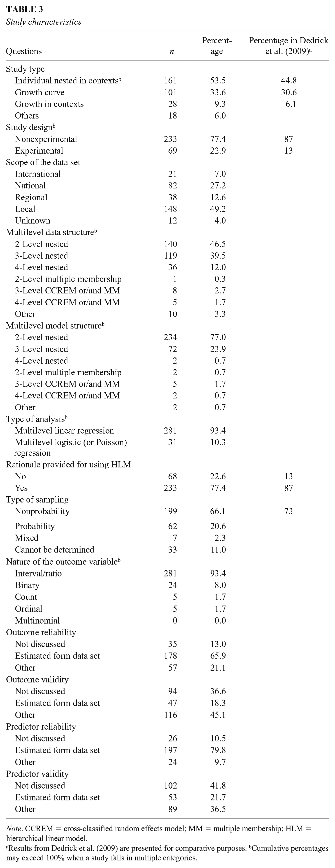
Table 3 shows the study characteristics. A variety of study types were found: 161 studies (53.5%) involved individuals nested in contexts; 101 studies (33.6%) involved repeated measures nested in individuals with the purpose of examining growth curves; 28 studies (9.3%) examined growth curves within contexts (i.e., repeated measures nested in individuals, which are further nested in contexts); and 18 studies (6.0%) involved repeated measures nested in individuals but did not model growth curves. The majority of the studies were nonexperimental (n = 233, 77.4%) and adopted nonprobability sampling approach (n = 199, 66.1%). Among the studies that used probability sampling (n = 69, 22.9%), more than half of them (n = 38, 55.1%) did not explicitly report whether sampling weights were used or at which level sampling weights were applied.

Table 3

Study characteristics

Questions	n	Percentage	Percentage in Dedrick et al. (2009)^a
Study type
Individual nested in contexts^b	161	53.5	44.8
Growth curve	101	33.6	30.6
Growth in contexts	28	9.3	6.1
Others	18	6.0
Study design^b
Nonexperimental	233	77.4	87
Experimental	69	22.9	13
Scope of the data set
International	21	7.0
National	82	27.2
Regional	38	12.6
Local	148	49.2
Unknown	12	4.0
Multilevel data structure^b
2-Level nested	140	46.5
3-Level nested	119	39.5
4-Level nested	36	12.0
2-Level multiple membership	1	0.3
3-Level CCREM or/and MM	8	2.7
4-Level CCREM or/and MM	5	1.7
Other	10	3.3
Multilevel model structure^b
2-Level nested	234	77.0
3-Level nested	72	23.9
4-Level nested	2	0.7
2-Level multiple membership	2	0.7
3-Level CCREM or/and MM	5	1.7
4-Level CCREM or/and MM	2	0.7
Other	2	0.7
Type of analysis^b
Multilevel linear regression	281	93.4
Multilevel logistic (or Poisson) regression	31	10.3
Rationale provided for using HLM
No	68	22.6	13
Yes	233	77.4	87
Type of sampling
Nonprobability	199	66.1	73
Probability	62	20.6
Mixed	7	2.3
Cannot be determined	33	11.0
Nature of the outcome variable^b
Interval/ratio	281	93.4
Binary	24	8.0
Count	5	1.7
Ordinal	5	1.7
Multinomial	0	0.0
Outcome reliability
Not discussed	35	13.0
Estimated form data set	178	65.9
Other	57	21.1
Outcome validity
Not discussed	94	36.6
Estimated form data set	47	18.3
Other	116	45.1
Predictor reliability
Not discussed	26	10.5
Estimated form data set	197	79.8
Other	24	9.7
Predictor validity
Not discussed	102	41.8
Estimated form data set	53	21.7
Other	89	36.5

Note. CCREM = cross-classified random effects model; MM = multiple membership; HLM = hierarchical linear model.

Results from Dedrick et al. (2009) are presented for comparative purposes. ^bCumulative percentages may exceed 100% when a study falls in multiple categories.

Most of the studies (n = 295, 98%) involved multilevel data with a strictly nested structure, among which 140 studies (46.5%) had two levels, 119 studies (39.5%) had three levels, and 36 studies (12.0%) had four levels. Only 4.7% of the studies (n = 14) involved multilevel data with a more complex structure such as the cross-classified and multiple membership data structure. Although less than half of the studies involved data with two levels, 77.7% of the studies (n = 234) fitted a two-level model. A much smaller proportion of studies fitted a three-level model (n = 72, 23.9%) or a four-level model (n = 2, 0.7%) or a cross-classified and/or multiple-membership model (n = 9, 3.0%). A closer examination reveals that some of the studies chose not to include the highest level because the variance components associated with the highest level (e.g., schools, districts, or other contexts) were not statistically significant. However, some studies simply ignored a level in three-level or four-level nested data or a crossed factor in cross-classified multilevel data, resulting in the disproportionately large number of two-level models. We found that only two studies provided justification for ignoring a higher level, which was due to small sample sizes.

In terms of sample sizes, most of the studies explicitly reported the number of units for each level (n = 295, 98.0%). For the studies with the individual-in-context design, the median number of the Level 1 to Level 4 units is 1,238 (ranged from 40 to 361,834), 71 (ranged from 4 to 23,710), 21 (ranged from 2 to 85), and 10 (ranged from 2 to 202), respectively. For the studies with the repeated-measure-in-individual design, the median sample size at each level is 4 repeated measures per individual (ranged from 2 to 54), 378 individuals (ranged from 2 to 241,114), 36 Level 3 units (ranged from 2 to 5,659), and 15 Level 4 units (ranged from 2 to 1,650), respectively.

In terms of the nature of the outcome, 281 studies (93.4%) had continuous outcomes while 34 studies (11.3%) had binary, count, or ordinal outcomes. The analysis type was generally consistent with the nature of the outcome. Specifically, 281 studies (93.4%) used LMMs and 31 studies (10.3%) nonnormal GLMMs such as multilevel logistic or multilevel Poisson regression analysis. However, a small portion of studies (n = 3, 1.0%) fitted multilevel linear regression models to categorical outcomes.

Two hundred eighty-eight studies (95.7%) involved outcome and/or predictors that are operationalizations of latent constructs. However, not all of these studies provided information on the psychometric properties of the operationalizations. Specifically, 35 studies (13.0%) did not report reliability, and 94 studies (36.6%) did not report validity for outcome variables. For predictors, 26 studies (10.5%) did not report reliability, and 102 studies (41.8%) did not report validity.

Model Specification and Communication

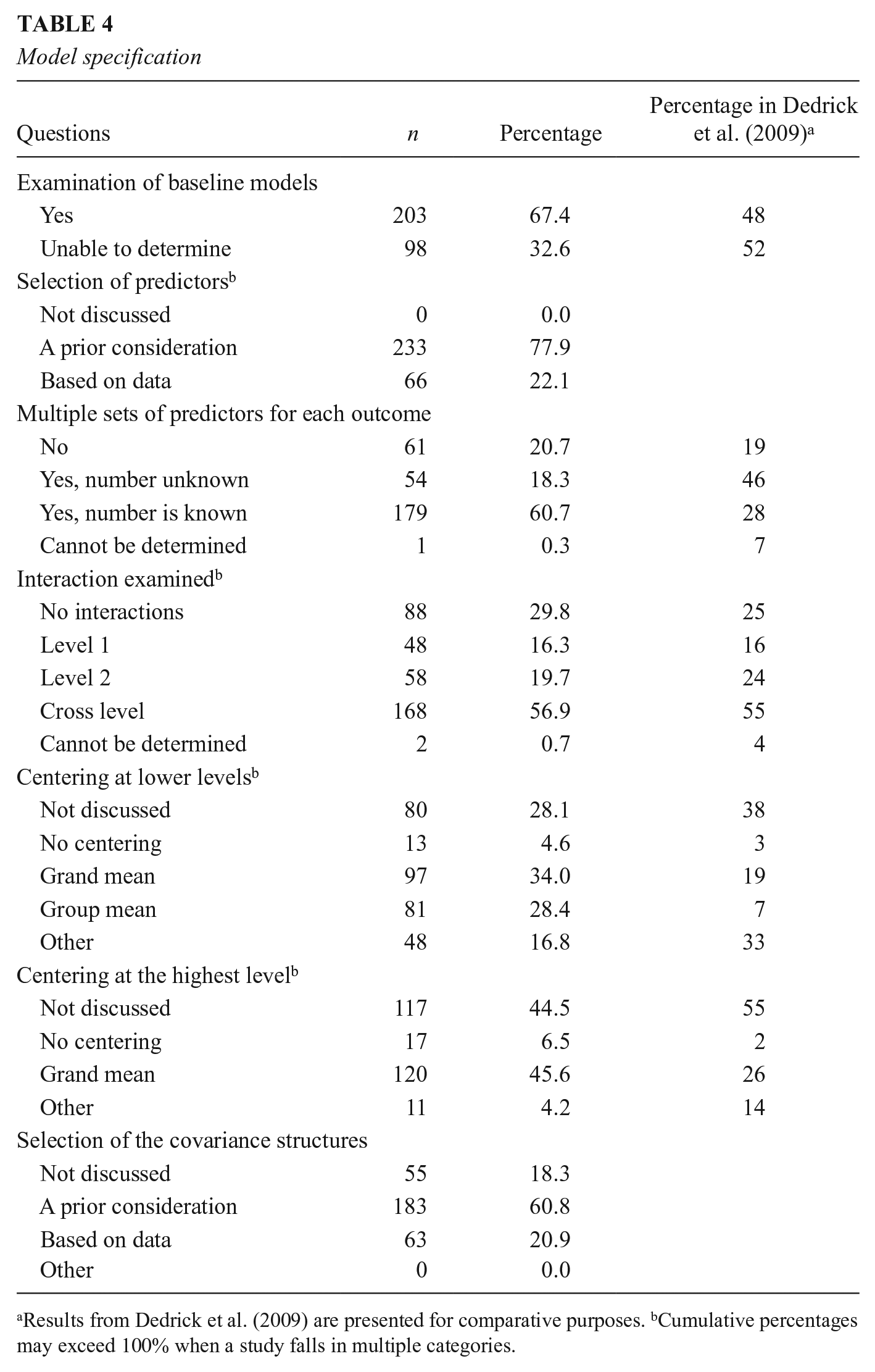
We were able to determine the exact number of models examined in a study for 80.1% (n = 241) of the sample. For the remaining studies, we cannot enumerate the models examined mainly because researchers conducted follow-up analyses in addition to the main analyses but did not provide explicit information about these additional models. The number of examined models ranged from 1 to 105, with a median of 7. Baseline models or unconditional models were explicitly examined and reported by 203 studies (67.4%).

For the selection of predictors, 233 studies (79.0%) had more than one set of predictors for each dependent variable, and 61 studies (20.7%) had only one set of predictors. Two hundred thirty-three studies (77.9%) selected predictors based on a priori considerations, while 66 studies (22.1%) selected predictors through a data-driven approach. The number of predictors in the most complicated model in a study ranged from 0 to 62, with a median of 12.

The majority of the studies tested interaction effects. Specifically, 48 studies (16.3%) examined Level 1 interactions; 58 studies (19.7%) examined higher-level interactions; 168 studies (56.9%) examined cross-level interactions; and two studies (0.7%) cannot be determined in terms of the type of interaction effects. Although not common, six studies (2.1%) tested cross-level interaction effects without including the main effects in the model, which could lead to biased estimates of the interaction effects. Moreover, 13 studies (4.3%) included a cross-level interaction but no random slope for the Level 1 predictor involved in the interaction.

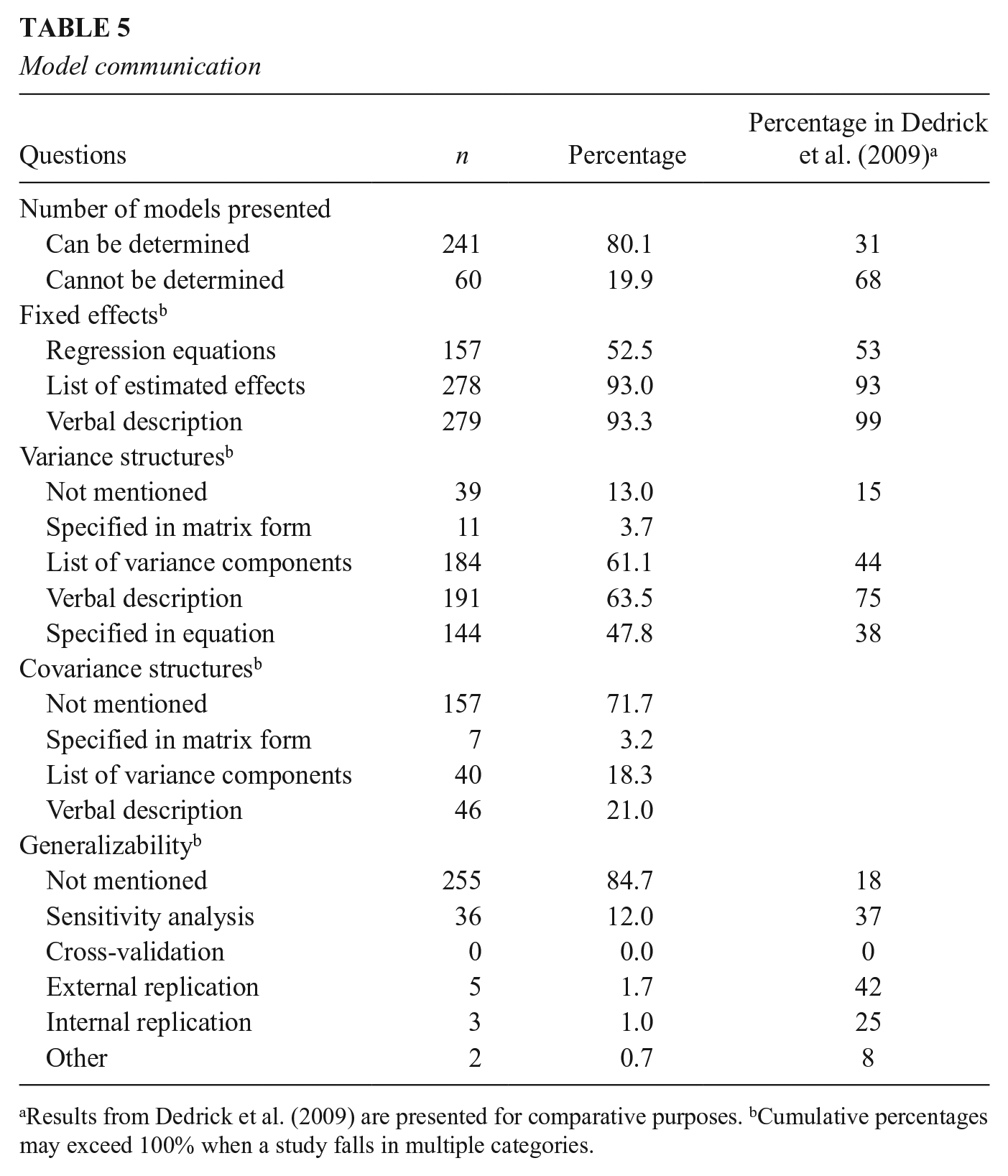
For the communication of fixed effects, most studies listed fixed effects in a results table (n = 278, 93.0%) and used verbal descriptions (n = 279, 93.3%). Regression equations were also used in many studies to show fixed effects specifications (n = 157, 52.5%). In addition to fixed effects, the specification of random effects is also a key element in MLMs. However, 39 studies (13.1%) did not provide any information on the specification of random effects. Among those that showed random effects specifications, verbal descriptions (n = 191, 63.5%) and listing of estimated variance components in a results table (n = 184, 61.1%) were the most prominent approaches, followed by regression equations (n = 144, 47.8%), while only 11 studies (3.7%) showed variance/covariance matrix of random effects. Fifty-five studies (18.3%) did not indicate how the decision regarding random effects specification was made. When this information was provided, we found that 183 studies (60.8%) determined the structures based on a priori considerations, while 63 studies (20.9%) used a data-driven approach. When there are multiple random effects at a higher level, most of the studies (n = 157, 71.7%) did not provide any information about the specification of covariances between the random effects.

Although centering has an implication for the interpretation of main effects and interaction effects in MLMs, 80 studies (28.1%) did not provide information about centering at lower levels and 117 studies (44.5%) did not provide any discussion about centering at the highest level. When centering was used at lower levels, researchers either used grand mean centering (n = 97, 34.0%) or group-mean centering (n = 81, 28.4%) or other approaches (n = 48, 16.8%) such as centering at a given time point in longitudinal data analyses. When centering was used at the highest level of a model, 117 studies (44.5%) adopted grand mean centering and 11 studies (4.2%) used other approaches such as centering on group means of higher-level clusters that exist in the data but are not included in the model or some forms of standardization.

Finally, for the generalizability of results, approaches such as sensitivity analysis, cross-validation, external replication/extension, and internal replication were coded. We found that 255 studies (84.7%) did not discuss generalizability, while only 46 studies (15.3%) provided evidence of generalizability using one or more of the approaches mentioned above. The results of reported information about model specification and communication are summarized in Tables 4 and 5, respectively.

Table 4

Model specification

Questions	n	Percentage	Percentage in Dedrick et al. (2009)^a
Examination of baseline models
Yes	203	67.4	48
Unable to determine	98	32.6	52
Selection of predictors^b
Not discussed	0	0.0
A prior consideration	233	77.9
Based on data	66	22.1
Multiple sets of predictors for each outcome
No	61	20.7	19
Yes, number unknown	54	18.3	46
Yes, number is known	179	60.7	28
Cannot be determined	1	0.3	7
Interaction examined^b
No interactions	88	29.8	25
Level 1	48	16.3	16
Level 2	58	19.7	24
Cross level	168	56.9	55
Cannot be determined	2	0.7	4
Centering at lower levels^b
Not discussed	80	28.1	38
No centering	13	4.6	3
Grand mean	97	34.0	19
Group mean	81	28.4	7
Other	48	16.8	33
Centering at the highest level^b
Not discussed	117	44.5	55
No centering	17	6.5	2
Grand mean	120	45.6	26
Other	11	4.2	14
Selection of the covariance structures
Not discussed	55	18.3
A prior consideration	183	60.8
Based on data	63	20.9
Other	0	0.0

Results from Dedrick et al. (2009) are presented for comparative purposes. ^bCumulative percentages may exceed 100% when a study falls in multiple categories.

Table 5

Model communication

Questions	n	Percentage	Percentage in Dedrick et al. (2009)^a
Number of models presented
Can be determined	241	80.1	31
Cannot be determined	60	19.9	68
Fixed effects^b
Regression equations	157	52.5	53
List of estimated effects	278	93.0	93
Verbal description	279	93.3	99
Variance structures^b
Not mentioned	39	13.0	15
Specified in matrix form	11	3.7
List of variance components	184	61.1	44
Verbal description	191	63.5	75
Specified in equation	144	47.8	38
Covariance structures^b
Not mentioned	157	71.7
Specified in matrix form	7	3.2
List of variance components	40	18.3
Verbal description	46	21.0
Generalizability^b
Not mentioned	255	84.7	18
Sensitivity analysis	36	12.0	37
Cross-validation	0	0.0	0
External replication	5	1.7	42
Internal replication	3	1.0	25
Other	2	0.7	8

Results from Dedrick et al. (2009) are presented for comparative purposes. ^bCumulative percentages may exceed 100% when a study falls in multiple categories.

Data Consideration

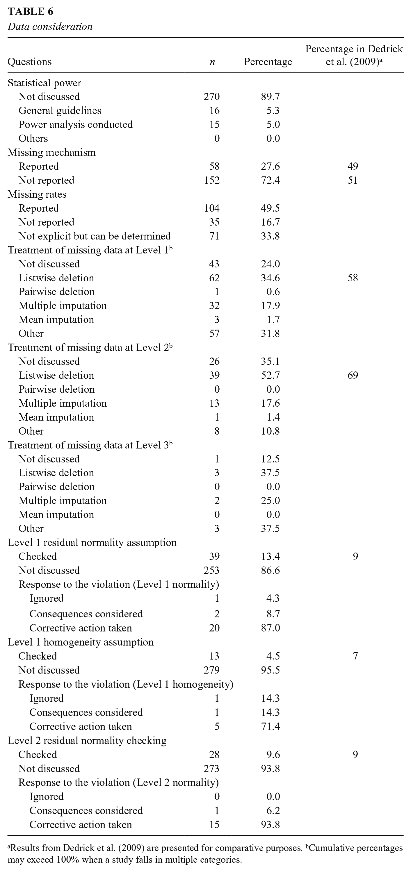
Like any statistical analysis, the validity of the statistical results from MLMs depends on the quality of the data. Hence, the consideration of statistical power, missing data, outliers, and underlying assumptions should not be overlooked. However, some of these issues are often not well addressed in empirical studies. In our sample, 270 studies (89.7%) had no discussion of power. Only 16 studies (5.3%) considered the general rules of sample size requirement, and even fewer studies (n = 15, 5.0%) conducted power analysis. On the other hand, missing data were addressed in the majority of the reviewed studies (n = 220, 73.1%). Specifically, 175 studies (83.3%) provided information about missing rates, but only 58 studies (27.6%) discussed the missing data mechanism (e.g., MCAR, MAR, and MNAR). One hundred seventy-nine studies (59.5%) reported having missing data at Level 1. Among these studies, listwise deletion (n = 62, 34.6%) and other approaches such as full information maximum likelihood (FIML) estimation (n = 57, 31.8%) are the most commonly used approaches, followed by multiple imputation (n = 32, 17.9%). Seventy-four studies (24.6%) reported having missing data at Level 2. Among these studies, the listwise deletion was the most commonly used approach (n = 39, 52.7%), followed by multiple imputation (n = 13, 17.6%). Only eight studies (2.7%) reported having missing data at Level 3, among which listwise deletion, multiple imputation, and other approaches such as FIML estimation were used with similar frequencies. It is noted that most multilevel modeling software with the exception of Mplus uses a conditional likelihood specification for FIML that can only handle missing data on the outcome variable but not on the predictor variables.

MLM diagnostics, including assumption checking and outlier screening, is a critical but often omitted step in the analyses of multilevel data. In our sample, only 39 studies (13.4%) checked the normality assumption of the Level 1 residuals and 13 studies (4.5%) checked the variance homogeneity of the Level 1 residuals. Only 28 studies (9.6%) checked the normality assumption of the Level 2 residuals. 27 studies (8.9%) found violations of assumptions, among which all but one studies either considered the consequences or took corrective actions to account for the violations. In the same vein, 270 studies (89.7%) did not provide evidence of screening of outliers and 284 studies (96.6%) did not consider the influences of unreliable measures. The results of reported information about data consideration are summarized in Table 6.

Table 6

Data consideration

Questions	n	Percentage	Percentage in Dedrick et al. (2009)^a
Statistical power
Not discussed	270	89.7
General guidelines	16	5.3
Power analysis conducted	15	5.0
Others	0	0.0
Missing mechanism
Reported	58	27.6	49
Not reported	152	72.4	51
Missing rates
Reported	104	49.5
Not reported	35	16.7
Not explicit but can be determined	71	33.8
Treatment of missing data at Level 1^b
Not discussed	43	24.0
Listwise deletion	62	34.6	58
Pairwise deletion	1	0.6
Multiple imputation	32	17.9
Mean imputation	3	1.7
Other	57	31.8
Treatment of missing data at Level 2^b
Not discussed	26	35.1
Listwise deletion	39	52.7	69
Pairwise deletion	0	0.0
Multiple imputation	13	17.6
Mean imputation	1	1.4
Other	8	10.8
Treatment of missing data at Level 3^b
Not discussed	1	12.5
Listwise deletion	3	37.5
Pairwise deletion	0	0.0
Multiple imputation	2	25.0
Mean imputation	0	0.0
Other	3	37.5
Level 1 residual normality assumption
Checked	39	13.4	9
Not discussed	253	86.6
Response to the violation (Level 1 normality)
Ignored	1	4.3
Consequences considered	2	8.7
Corrective action taken	20	87.0
Level 1 homogeneity assumption
Checked	13	4.5	7
Not discussed	279	95.5
Response to the violation (Level 1 homogeneity)
Ignored	1	14.3
Consequences considered	1	14.3
Corrective action taken	5	71.4
Level 2 residual normality checking
Checked	28	9.6	9
Not discussed	273	93.8
Response to the violation (Level 2 normality)
Ignored	0	0.0
Consequences considered	1	6.2
Corrective action taken	15	93.8

Results from Dedrick et al. (2009) are presented for comparative purposes. ^bCumulative percentages may exceed 100% when a study falls in multiple categories.

Estimation and Statistical Inferences

About two thirds of the studies (n = 203, 67.4%) reported the software used for their analyses. The majority of the studies (n = 101, 49.5%) used HLM, followed sequentially by SAS (n = 34, 16.7%), Mplus (n = 23, 11.3%), SPSS (n = 14, 6.9%), R (n = 13, 6.4%), MLwiN (n = 10, 4.9%), and Stata (n = 8, 3.9%).

Computational aspects such as estimation methods, algorithms, convergence issues, and nonpositive definite matrices were usually ignored in empirical studies. In our sample, 99 studies (32.9%) reported estimation methods, while only five studies (1.7%) reported algorithms and 13 studies (4.3%) reported whether the estimation converged or not. For LMMs, 95 out of 281 studies reported estimation methods. The most commonly used estimation method was FML (n = 69, 72.6%),¹ followed by REML (n = 23, 24.2%), Bayesian approach (n = 3, 3.2%). For nonnormal GLMMs, only four out of 31 studies reported estimation methods, namely, PQL (n = 3, 75.0%) and Bayesian approach (n = 1, 25.0%). None of the studies reported encountering nonpositive definite matrices. The results of reported information about computational issues are summarized in Table 7.

Table 7

Computational issues

Questions	n	Percentage	Percentage in Dedrick et al. (2009)^a
Software	203	67.4	48
HLM	101	49.8	70
SAS	34	16.7	23
Mplus	23	11.3
SPSS	14	6.9
R	13	6.4
MLwiN	10	4.9
Stata	8	3.9
Estimation method for LMM
Not reported	186	66.2
Reported	95	33.8
FML	69	75.3	47
REML	23	21.3	20
Bayesian approach	3	3.2	20
Estimation method for nonnormal GLMM
Not reported	27	87.1
Reported	4	12.9
PQL	3	75.0
Bayesian approach	1	25.0
Estimation algorithm reported	5	1.7	1
Convergence issues reported	13	4.3	2
Nonpositive definite issues reported	0	0.0	1

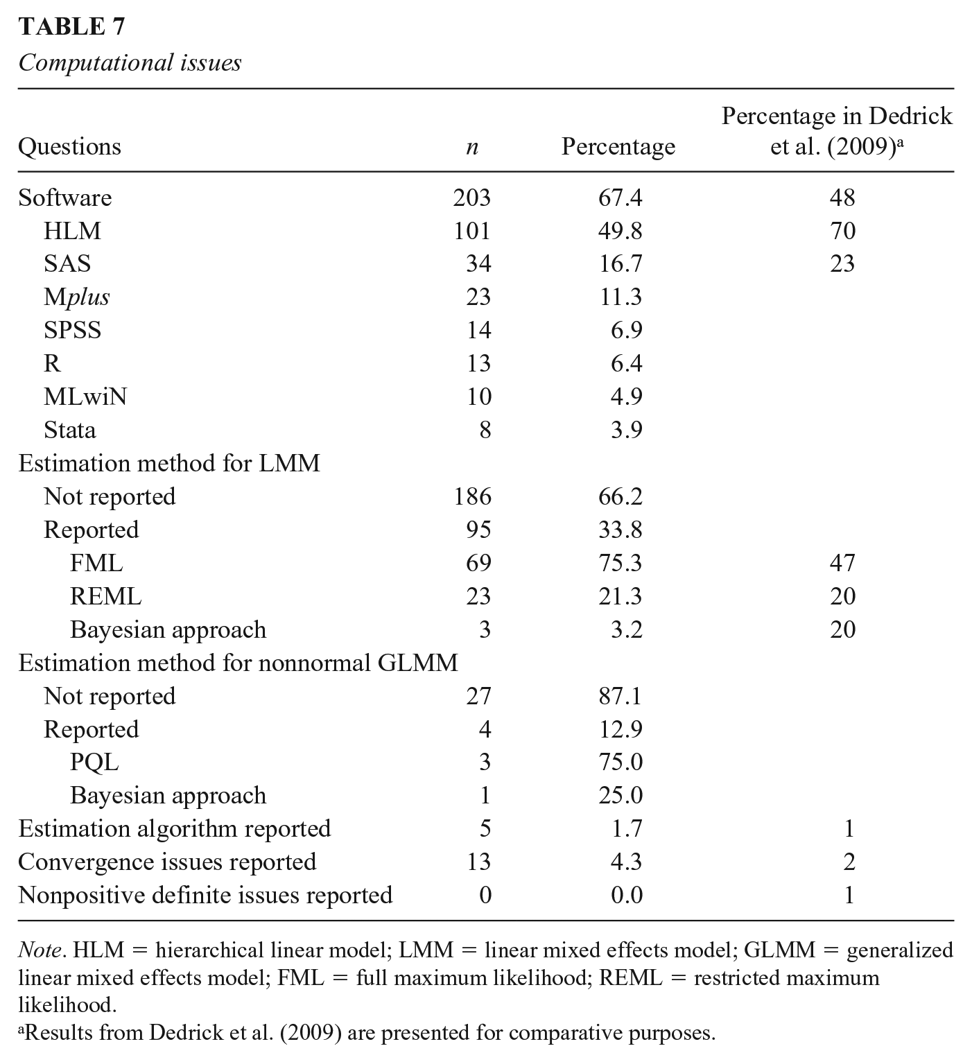
Note. HLM = hierarchical linear model; LMM = linear mixed effects model; GLMM = generalized linear mixed effects model; FML = full maximum likelihood; REML = restricted maximum likelihood.

Results from Dedrick et al. (2009) are presented for comparative purposes.

When reporting estimates for fixed effects, most of the studies included point estimates (n = 292, 97.0%) and significance tests (n = 289, 96.0%). However, slightly fewer studies reported standard errors (n = 248, 82.4%) and very few studies (n = 23, 7.6%) reported confidence intervals for the fixed effects. In studies that reported significance tests and/or confidence intervals (n = 293), 180 (61.4%) did not mention the method used for making the inferences and 90 (30.7%) just provided partial information such as reporting t-test or F-test results without providing the method of computing degrees of freedom.

The reporting of variance component estimates was less satisfactory than that of fixed effects. About 36.9% of the studies (n = 111) did not provide any information on variance component estimates. Among studies that provided variance component estimates (n = 190), 168 (56.4%) reported estimates for the variance of a random intercept, 112 (48.9%) reported estimates for the variance of a random slope, and 143 (50.4%) reported residual variance. Only 26 studies (11.8%) provided the estimates of covariances or correlations between a random intercept and a random slope. Due to the lack of information in specifications of random effects, it is hard to determine whether the covariances were constrained as zero in the models or there was underreporting for the covariances. In addition to point estimates, 150 studies (49.8%) reported significance tests, 81 studies (26.9%) reported standard errors, 93 studies (30.9%) reported intraclass correlations, and 64 studies (21.3%) reported explained variances. Again, confidence intervals were seldom reported (n = 10, 3.3%). In the subset (n = 157) where significance tests and/or confidence intervals were provided, 89 studies (56.7%) did not mention the method used for making the inferences of variance components.

Finally, effect sizes are important measures of the practical significance of the findings. However, nearly half of the studies (n = 136, 45.2%) did not report any effect size. The most commonly used effect size measure is the proportion of variance explained (21.6%), followed by the standardized regression coefficient (15.0%). As shown in the previous section, 233 studies (79.0%) tested multiple models, therefore it is important to show how the different models fit the data. However, in our sample, most of the studies (n = 196, 65.1%) did not report any model fit index. When it was reported, deviance is the most commonly used measure (n = 85, 28.2%), followed by AIC (n = 44, 14.6%) and BIC (n = 33, 11.0%). The results of reported information about estimation, inferences, and model fit are summarized in Table 8.

Table 8

Estimation, inferences, and model fit

Questions	n	Percentage	Percentage in Dedrick et al. (2009)^a
Fixed effects information^b
None	6	2.0	2
Point estimates	292	97.0	97
Standard errors	248	82.4	59
Confidence intervals	23	7.6	4
Significance tests	289	96.0	97
Other	6	2.0	36
Variance components information^b
None	60	19.9	23
Point estimates	190	63.1	49
Standard errors	81	26.9	4
Confidence intervals	10	3.3	0
Significance tests	150	49.8	63
Reliabilities	7	2.3	22
Intraclass correlations	93	30.9	22
Explained variances	64	21.3	39
Random effects estimate information
None	292	97.0	94
EB or OLS estimates	6	2.0	2
Provided but method not stated	3	1.0
Effect size information^b
None	136	45.2
Proportion of variance explained	65	21.6
Standardized coefficient	45	15.0
Cohen’s d	28	9.3
Odds ratio	13	4.3
Other	55	18.3
Model fit index^b
None	196	65.1
AIC	44	14.6
BIC	33	11.0
Deviance	85	28.2
DIC	1	0.3
Other	7	2.3

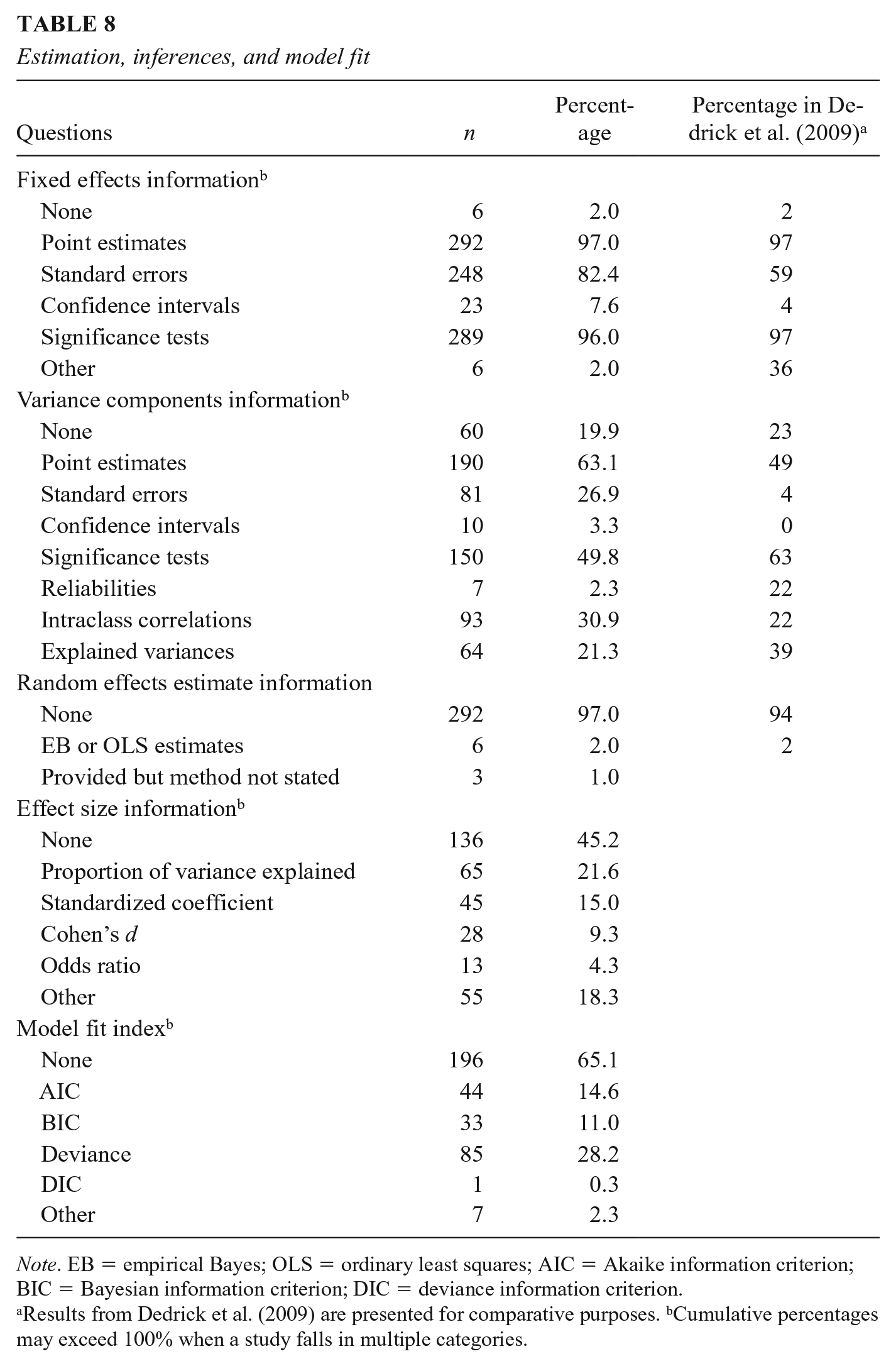
Note. EB = empirical Bayes; OLS = ordinary least squares; AIC = Akaike information criterion; BIC = Bayesian information criterion; DIC = deviance information criterion.

Results from Dedrick et al. (2009) are presented for comparative purposes. ^bCumulative percentages may exceed 100% when a study falls in multiple categories.

Discussion and Conclusion

We reviewed the practices of reporting studies that employed multilevel modeling techniques (i.e., LMM and nonnormal GLMM) over the past 10 years in light of new methodological advancement in the field. Compared with the findings of the earlier review (Dedrick et al., 2009), we are pleased to see improvements in several areas. Researchers are clearer in reporting the number of models tested as well as the number of different sets of predictors for each outcome. The centering of predictors is more explicitly stated. When dealing with missing data, researchers use more advanced techniques such as FIML estimation and multiple imputation rather than listwise deletion. A higher proportion of studies explicitly report the software used. Finally, more information is provided for the estimates of variance components, including point estimates and standard error estimates.

However, some poor practices persist. In terms of model specification, the majority of the studies failed to provide rationales for random effects. Underspecification is an issue as researchers tend to ignore a level in the data or simply assume fixed slopes even when the design requires random slopes (e.g., when testing cross-level interactions). When there are multiple random effects at a level, most studies did not explicitly state the covariance structure of the random effects. In terms of data considerations, although missing data are prevalent, only a small proportion of studies discussed missing mechanisms. Power analyses, assumption checking, and outlier screening were rarely mentioned. In terms of model results, more than 60% of studies failed to provide model fit indexes when multiple models were compared, and only half of the studies provided some sort of effect size measures.

Hence, we iterate the reporting guidelines for MLM by Dedrick et al. (2009) and include three additional recommendations in light of the updated journal article reporting standards for quantitative research by the American Psychological Association (Appelbaum et al., 2018) and the findings of this review.

Provide a clear description of how the presented models were developed, such as the process of selecting the predictors and the covariance structure, and the number of models examined. Supplemental materials showing model specifications in equations and/or software syntax are recommended.

Explicitly describe centering procedures with information on whether centering was applied, which variables were centered, and what types of methods were used.

State clear descriptions of how statistical assumptions (i.e., data distributions at each level) were checked and how outliers were screened.

Discuss the mechanism for missing data and possible effects of the missingness on the results when applicable.

Provide details on the analysis methods by indicating the software and version used, estimation method chosen, and any possible estimation issue, such as nonconvergence and nonpositive definite covariance matrices.

Report all parameter estimates such as fixed effects and variance parameters for any tested models and provide either standard errors or interval estimates for the parameters of interest.

Explicitly describe the statistical power of an inferential test in MLMs. The determination of sample size should be based on specific power analyses, rather than on the general sample size requirement guidelines.

Provide effect size estimates and confidence intervals on the main parameter estimates in addition to the significance test.

Report reliability and validity of measures based on the levels with which the underlying constructs are associated with.

Finally, for future research and teaching of MLM, one area that applied researchers need more guidance on is how to specify random effects structures. The performance of the maximal approach and the model selection approach needs to be further evaluated in models with more levels and more predictors as well as under data conditions that are not ideal, such as small sample sizes and assumption violations. As indicated by our review, the underspecification of random effects structures is an issue. Step-by-step tutorials will be helpful to guide applied researchers through the process of finding the best random effects structure.

Supplemental Material

sj-docx-1-rer-10.3102_0034654321991229 – Supplemental material for Reporting Practice in Multilevel Modeling: A Revisit After 10 Years

Supplemental material, sj-docx-1-rer-10.3102_0034654321991229 for Reporting Practice in Multilevel Modeling: A Revisit After 10 Years by Wen Luo, Haoran Li, Eunkyeng Baek, Siqi Chen, Kwok Hap Lam and Brandie Semma in Review of Educational Research

Supplemental Material

sj-docx-2-rer-10.3102_0034654321991229 – Supplemental material for Reporting Practice in Multilevel Modeling: A Revisit After 10 Years

Supplemental material, sj-docx-2-rer-10.3102_0034654321991229 for Reporting Practice in Multilevel Modeling: A Revisit After 10 Years by Wen Luo, Haoran Li, Eunkyeng Baek, Siqi Chen, Kwok Hap Lam and Brandie Semma in Review of Educational Research

Footnotes

Notes

Authors

WEN LUO is an associate professor in the Research, Measurement, and Statistics Program, Department of Educational Psychology Department, Texas A&M University, 4225 TAMU, College Station, TX 77843, USA; email: wluo@tamu.edu . Her research interests include multilevel modeling, structural equation modeling, and the applications of these techniques in longitudinal data analyses.

HAORAN LI is a doctoral student in the Research, Measurement, and Statistics Program, Department of Educational Psychology, Texas A&M University, 4225 TAMU, College Station, TX 77843, USA; email: haoran@tamu.edu . Methodologically, he is interested in multilevel modeling, structural equation modeling, and longitudinal analysis. He is also interested in the longitudinal development of cognitive ability and changes in academic motivation.

EUNKYENG BAEK is an assistant professor in the Research, Measurement, and Statistics Program, Department of Educational Psychology Department, Texas A&M University, 4225 TAMU, College Station, TX 77843, USA; email: baek@tamu.edu . Her research interests include multilevel modeling using single-case experimental data, Bayesian estimation, and the applications of these techniques in educational and psychological data.

SIQI CHEN is a psychometrician at Pearson, 19500 Bulverde Road, San Antonio, TX 78259, USA; email: siqi.chen@pearson.com . Her research interests include causal inference, multilevel modeling, and data mining techniques.

KWOK HAP LAM is a doctoral student in the Research, Measurement, and Statistics Program, Department of Educational Psychology Department, Texas A&M University, 4225 TAMU, College Station, TX 77843,USA; email: amy_hap07@tamu.edu . Her research interests include single-case data analysis and multilevel modeling.

BRANDIE SEMMA is a doctoral student in the Research Methods and Statistics Program, Department of Educational Psychology Department, Texas A&M University, 4225 TAMU, College Station, TX 77843, USA; email: brandiesemma@tamu.edu . Her research interests include meta-analysis, missing data techniques, and Bayesian analysis.

References

Agresti

Caffo

Ohman-Strickland

(2004). Examples in which misspecification of a random effects distribution reduces efficiency, and possible remedies. Computational Statistics & Data Analysis, 47(3), 639–653. https://doi.org/10.1016/j.csda.2003.12.009

Agresti

Natarajan

(2001). Modeling clustered ordered categorical data: A survey. International Statistical Review, 69(3), 345–371. https://doi.org/10.1111/j.1751-5823.2001.tb00463.x

Appelbaum

Cooper

Kline

R. B.

Mayo-Wilson

Nezu

A. M.

Rao

S. M.

(2018). Journal article reporting standards for quantitative research in psychology: The APA publications and communications board task force report. American Psychologist, 73(1), 3–25. https://doi.org/10.1037/amp0000191

Arend

M. G.

Schäfer

(2019). Statistical power in two-level models: A tutorial based on Monte Carlo simulation. Psychological Methods, 24(1), 1–19. https://doi.org/10.1037/met0000195

Baayen

R. H.

Davidson

D. J.

Bates

D. M.

(2008). Mixed-effects modeling with crossed random effects for subjects and items. Journal of Memory and Language, 59(4), 390–412. https://doi.org/10.1016/j.jml.2007.12.005

Baldwin

S. A.

Bauer

D. J.

Stice

Rohde

(2011). Evaluating models for partially clustered designs. Psychological Methods, 16(2), 149–165. https://doi.org/10.1037/a0023464

Baldwin

S. A.

Fellingham

G. W.

(2013). Bayesian methods for the analysis of small sample multilevel data with a complex variance structure. Psychological Methods, 18(2), 151–164. https://doi.org/10.1037/a0030642

Barr

D. J.

(2013). Random effects structure for testing interactions in linear mixed-effects models. Frontiers in Psychology, 4, Article 328. https://doi.org/10.3389/fpsyg.2013.00328

Barr

D. J.

Levy

Scheepers

Tily

H. J.

(2013). Random effects structure for confirmatory hypothesis testing: Keep it maximal. Journal of Memory and Language, 68(3), 255–278. https://doi.org/10.1016/j.jml.2012.11.001

10.

Bates

Mächler

Bolker

Walker

(2015). Fitting linear mixed-effects models using lme4. Journal of Statistical Software, 67(1), 1–48. https://doi.org/10.18637/jss.v067.i01

11.

Bates

M. D.

Castellano

K. E.

Rabe-Hesketh

Skrondal

(2014). Handling correlations between covariates and random slopes in multilevel models. Journal of Educational and Behavioral Statistics, 39(6), 524–549. https://doi.org/10.3102/1076998614559420

12.

Bauer

D. J.

Cai

(2009). Consequences of unmodeled nonlinear effects in multilevel models. Journal of Educational and Behavioral Statistics, 34(1), 97–114. https://doi.org/10.3102/1076998607310504

13.

Bauer

D. J.

Sterba

S. K.

(2011). Fitting multilevel models with ordinal outcomes: Performance of alternative specifications and methods of estimation. Psychological Methods, 16(4), 373–390. https://doi.org/10.1037/a0025813

14.

Bell

B. A.

Morgan

G. B.

Schoeneberger

J. A.

Kromrey

J. D.

Ferron

J. M.

(2014). How low can you go? An investigation of the influence of sample size and model complexity on point and interval estimates in two-level linear models. Methodology, 10(1), 1–11. https://doi.org/10.1027/1614-2241/a000062

15.

Berkhof

Snijders

T. A.

(2001). Variance component testing in multilevel models. Journal of Educational and Behavioral Statistics, 26(2), 133–152. https://doi.org/10.3102/10769986026002133

16.

Brauer

Curtin

J. J.

(2018). Linear mixed-effects models and the analysis of nonindependent data: A unified framework to analyze categorical and continuous independent variables that vary within-subjects and/or within-items. Psychological Methods, 23(3), 389–411. https://doi.org/10.1037/met0000159

17.

Breslow

N. E.

Clayton

D. G.

(1993). Approximate inference in generalized linear mixed models. Journal of the American Statistical Association, 88(421), 9–25. https://doi.org/10.1080/01621459.1993.10594284

18.

Breslow

N. E.

Lin

(1995). Bias correction in generalized linear mixed models with a single component of dispersion. Biometrika, 82(1), 81–91. https://doi.org/10.1093/biomet/82.1.81

19.

Browne

W. J.

(2019). MCMC estimation in MLwiN Version 3.03. Centre for Multilevel Modelling, University of Bristol.

20.

Browne

W. J.

Draper

(2006). A comparison of Bayesian and likelihood-based methods for fitting multilevel models. Bayesian Analysis, 1(3), 473–514. https://doi.org/10.1214/06-BA117

21.

Bryk

A. S.

Raudenbush

S. W.

(1992). Hierarchical linear models: Applications and data analysis methods. Sage.

22.

Bürkner

P. C.

(2017). Advanced Bayesian multilevel modeling with the R package brms. The R Journal, 10/1(July), 395–411. https://doi.org/10.32614/RJ-2018-017

23.

Capanu

Gὄnen

Begg

C. B.

(2013). An assessment of estimation methods for generalized linear mixed models with binary outcomes. Statistics in Medicine, 32(26), 4550–4566. https://doi.org/10.1002/sim.5866

24.

Carroll

Lawson

A. B.

Faes

Kirby

R. S.

Aregay

Watjou

(2015). Comparing INLA and OpenBUGS for hierarchical Poisson modeling in disease mapping. Spatial and Spatio-Temporal Epidemiology, 14–15(July–October), 45–54. https://doi.org/10.1016/j.sste.2015.08.001

25.

Cho

S. J.

Rabe-Hesketh

(2011). Alternating imputation posterior estimation of models with crossed random effects. Computational Statistics & Data Analysis, 55(1), 12–25. https://doi.org/10.1016/j.csda.2010.04.015

26.

Chung

Beretvas

S. N.

(2012). The impact of ignoring multiple membership data structures in multilevel models. British Journal of Mathematical and Statistical Psychology, 65(2), 185–200. https://doi.org/10.1111/j.2044-8317.2011.02023.x

27.

Crainiceanu

C. M.

Ruppert

(2004). Likelihood ratio tests in linear mixed models with one variance component. Journal of the Royal Statistical Society: Series B: Statistical Methodology, 66(1), 165–185. https://doi.org/10.1111/j.1467-9868.2004.00438.x

28.

Dedrick

R. F.

Ferron

J. M.

Hess

M. R.

Hogarty

K. Y.

Kromrey

J. D.

Lang

T. R.

Niles

J. D.

Lee

R. S.

(2009). Multilevel modeling: A review of methodological issues and applications. Review of Educational Research, 79(1), 69–102. https://doi.org/10.3102/0034654308325581

29.

Depaoli

Van de Schoot

(2017). Improving transparency and replication in Bayesian statistics: The WAMBS-Checklist. Psychological Methods, 22(2), 240–261. https://doi.org/10.1037/met0000065

30.

Dong

Kelcey

Spybrook

Maynard

R. A.

(2017). PowerUp!-Moderator: A tool for calculating statistical power and minimum detectable effect size of the moderator effects in cluster randomized trials (Version 1.08) [Computer software]. Casual Evaluation. http://www.causalevaluation.org/

31.

Dong

Maynard

R. A.

(2013). PowerUp! A tool for calculating minimum detectable effect sizes and minimum required sample sizes for experimental and quasi-experimental design studies. Journal of Research on Educational Effectiveness, 6(1), 24–67. https://doi.org/10.1080/19345747.2012.673143

32.

Donohue

M. C.

Gamst

A. C.

Edland

S. D.

Donohue

(2013). Package “longpower.” Biometrics, 53, 937–947.

33.

Fang

Wong

W. K.

(2016). Detecting the violation of variance homogeneity in mixed models. Statistical Methods in Medical Research, 25(6), 2506–2520. https://doi.org/10.1177/0962280214526194

34.

Ferron

Dailey

(2002). Effects of misspecifying the first-level error structure in two-level models of change. Multivariate Behavioral Research, 37(3), 379–403. https://doi.org/10.1207/S15327906MBR3703_4

35.

Finch

(2017). Multilevel modeling in the presence of outliers: A comparison of robust estimation methods. Psicologica: International Journal of Methodology and Experimental Psychology, 38(1), 57–92.

36.

Fournier

D. A.

Skaug

H. J.

Ancheta

Ianelli

Magnusson

Maunder

M. N.

Nielsen

Sibert

(2012). AD Model Builder: Using automatic differentiation for statistical inference of highly parameterized complex nonlinear models. Optimization Methods & Software, 27(2), 233–249. https://doi.org/10.1080/10556788.2011.597854

37.

Geldhof

G. J.

Preacher

K. J.

Zyphur

M. J.

(2014). Reliability estimation in a multilevel confirmatory factor analysis framework. Psychological Methods, 19(1), 72–91. https://doi.org/10.1037/a0032138

38.

Gelman

(2006). Prior distributions for variance parameters in hierarchical models (comment on article by Browne and Draper). Bayesian Analysis, 1(3), 515–534. https://doi.org/10.1214/06-BA117A

39.

Goldstein

(1986). Multilevel mixed linear model analysis using iterative generalized least squares. Biometrika, 73(1), 43–56. https://doi.org/10.1093/biomet/73.1.43

40.

Green

MacLeod

C. J.

(2016). SIMR: An R package for power analysis of generalized linear mixed models by simulation. Methods in Ecology and Evolution, 7(4), 493–498. https://doi.org/10.1111/2041-210X.12504

41.

Hadfield

J. D.

(2010). MCMC methods for multi-response generalized linear mixed models: The MCMCglmm R package. Journal of Statistical Software, 33(2), 1–22. https://doi.org/10.18637/jss.v033.i02

42.

Hedeker

(2008). Multilevel models for ordinal and nominal variables. In de Leeuw

Meijer

(Eds.), Handbook of multilevel analysis (pp. 237–274). Springer. https://doi.org/10.1007/978-0-387-73186-5_6

43.

Hedges

L. V.

(2007). Effect sizes in cluster-randomized designs. Journal of Educational and Behavioral Statistics, 32(4), 341–370. https://doi.org/10.3102/1076998606298043

44.

Hedges

L. V.

(2011). Effect sizes in three-level cluster randomized experiments. Journal of Educational and Behavioral Statistics, 36(3), 346–380. https://doi.org/10.3102/1076998610376617

45.

Heisig

J. P.

Schaeffer

(2019). Why you should always include a random slope for the lower-level variable involved in a cross-level interaction. European Sociological Review, 35(2), 258–279. https://doi.org/10.1093/esr/jcy053

46.

Halekoh

Højsgaard

(2014). A Kenward-Roger approximation and parametric bootstrap methods for tests in linear mixed models: The R package pbkrtest. Journal of Statistical Software, 59(9), 1–30. https://doi.org/10.18637/jss.v059.i09

47.

Hox

J. J.

(1998). Multilevel modeling: When and why. In Balderjahn

Mathar

Schader

(Eds.), Classification, data analysis, and data highways (pp. 147–154). Springer. https://doi.org/10.1007/978-3-642-72087-1_17

48.

Hox

J. J.

Moerbeek

Van de Schoot

(2010). Multilevel analysis: Techniques and applications (2nd ed.). Routledge.

49.

Joe

(2008). Accuracy of Laplace approximation for discrete response mixed models. Computational Statistics & Data Analysis, 52(12), 5066–5074. https://doi.org/10.1016/j.csda.2008.05.002

50.

Kass

R. E.

Natarajan

(2006). A default conjugate prior for variance components in generalized linear mixed models (comment on article by Browne and Draper). Bayesian Analysis, 1(3), 535–542. https://doi.org/10.1214/06-BA117B

51.

Kelcey

Dong

Spybrook

Shen

(2017). Experimental power for indirect effects in group-randomized studies with group-level mediators. Multivariate Behavioral Research, 52(6), 699–719. https://doi.org/10.1080/00273171.2017.1356212

52.

Kelley

Preacher

K. J.

(2012). On effect size. Psychological Methods, 17(2), 137–152. https://doi.org/10.1037/a0028086

53.

Kenward

M. G.

Roger

J. H.

(1997). Small sample inference for fixed effects from restricted maximum likelihood. Biometrics, 53(3), 983–997. https://doi.org/10.2307/2533558

54.

Kenward

M. G.

Roger

J. H.

(2009). An improved approximation to the precision of fixed effects from restricted maximum likelihood. Computational Statistics & Data Analysis, 53(7), 2583–2595. https://doi.org/10.1016/j.csda.2008.12.013

55.

Keselman

Algina

Kowalchunk

Wolfinger

(1998). A comparison of two approaches for selecting covariance structures in the analysis of repeated measurements. Communications in Statistics: Simulation and Computation, 27(3), 591–604. https://doi.org/10.1080/03610919808813497

56.

Kim

E. S.

Dedrick

R. F.

Cao

Ferron

J. M.

(2016). Multilevel factor analysis: Reporting guidelines and a review of reporting practices. Multivariate Behavioral Research, 51(6), 881–898. https://doi.org/10.1080/00273171.2016.1228042

57.

Kim

J. S.

Frees

E. W.

(2007). Multilevel modeling with correlated effects. Psychometrika, 72(4), 505–533. https://doi.org/10.1007/s11336-007-9008-1

58.

Kloke

McKean

J. W.

(2014). Nonparametric statistical methods using R. CRC Press. https://doi.org/10.1201/b17501

59.

Kloke

J. D.

McKean

J. W.

Rashid

M. M.

(2009). Rank-based estimation and associated inferences for linear models with cluster correlated errors. Journal of the American Statistical Association, 104(485), 384–390. https://doi.org/10.1198/jasa.2009.0116

60.

Kreft

I. G. G.

(1996). Are multilevel techniques necessary? An overview, including simulation studies. California State University, Los Angeles.

61.

Kuznetsova

Brockhoff

P. B.

Christensen

R. H. B.

(2017). lmerTest package: Tests in linear mixed effects models. Journal of Statistical Software, 82(13), 1–26. https://doi.org/10.18637/jss.v082.i13

62.

Kwok

West

Green

(2007). The impact of misspecifying the within-subject covariance structure in multiwave longitudinal multilevel models: A Monte Carlo study. Multivariate Behavioral Research, 42(3), 557–592. https://doi.org/10.1080/00273170701540537

63.

Lai

M. H. C.

(2018, December 3). bootmlm: Bootstrap resampling for multilevel models (R Package Version 0.0.1) [Computer software]. Zenodo. https://doi.org/10.5281/zenodo.1879127

64.

Lai

M. H. C.

(2020a). Bootstrap confidence intervals for multilevel standardized effect size. Multivariate Behavioral Research. Advance online publication. https://doi.org/10.1080/00273171.2020.1746902

65.

Lai

M. H. C.

(2020b). Composite reliability of multilevel data: It’s about observed scores and construct meanings. Psychological Methods. Advance online publication. https://doi.org/10.1037/met0000287

66.

Lai

M. H. C.

Kwok

O. M.

(2014). Standardized mean differences in two-level cross-classified random effects models. Journal of Educational and Behavioral Statistics, 39(4), 282–302. https://doi.org/10.3102/1076998614532950

67.

Lai

M. H. C.

Kwok

O. M.

(2015). Examining the rule of thumb of not using multilevel modeling: The “design effect smaller than two” rule. Journal of Experimental Education, 83(3), 423–438. https://doi.org/10.1080/00220973.2014.907229

68.

Lai

M. H. C.

Kwok

O. M.

(2016). Estimating standardized effect sizes for two-and three-level partially nested data. Multivariate Behavioral Research, 51(6), 740–756. https://doi.org/10.1080/00273171.2016.1231606

69.

Landau

Stahl

(2013). Sample size and power calculations for medical studies by simulation when closed form expressions are not available. Statistical Methods in Medical Research, 22(3), 324–345. https://doi.org/10.1177/0962280212439578

70.

Lane

S. P.

Hennes

E. P.

(2018). Power struggles: Estimating sample size for multilevel relationships research. Journal of Social and Personal Relationships, 35(1), 7–31. https://doi.org/10.1177/0265407517710342

71.

Lange

K. L.

Little

R. J.

Taylor

J. M.

(1989). Robust statistical modeling using the t distribution. Journal of the American Statistical Association, 84(408), 881–896. https://doi.org/10.2307/2290063

72.

LeBeau

(2016). Impact of serial correlation misspecification with the linear mixed model. Journal of Modern Applied Statistical Methods, 15(1), 389–416. https://doi.org/10.22237/jmasm/1462076400

73.

Leckie

Browne

Goldstein

Merlo

Austin

(2019, April). Variance partitioning in multilevel models for count data [Paper presentation]. 12th International Multilevel Conference, Utrecht, Netherlands. https://arxiv.org/ftp/arxiv/papers/1911/1911.06888.pdf

74.

Lee

Grimm

K. J.

(2018). Generalized linear mixed-effects modeling programs in R for binary outcomes. Structural Equation Modeling: A Multidisciplinary Journal, 25(5), 824–828. https://doi.org/10.1080/10705511.2018.1500141

75.

Lindstrom

M. J.

Bates

D. M.

(1988). Newton-Raphson and EM algorithms for linear mixed-effects models for repeated-measures data. Journal of the American Statistical Association, 83(404), 1014–1022. https://doi.org/10.1080/01621459.1988.10478693

76.

Liu

Zhang

Grimm

K. J.

(2016). Comparison of inverse Wishart and separation-strategy priors for Bayesian estimation of covariance parameter matrix in growth curve analysis. Structural Equation Modeling: A Multidisciplinary Journal, 23(3), 354–367. https://doi.org/10.1080/10705511.2015.1057285

77.

Liu

Agresti

(2005). The analysis of ordered categorical data: An overview and a survey of recent developments. Test, 14(1), 1–73. https://doi.org/10.1007/BF02595397

78.

Loy

(2016). Package HLMdiag (Version 0.4.0) [Computer software]. http://cran.r-project.org/web/packages/HLMdiag/HLMdiag.pdf

79.

Tang

Crits-Christoph

Zhang

(2009). On the impact of parametric assumptions and robust alternatives for longitudinal data analysis. Biometrical Journal: Journal of Mathematical Methods in Biosciences, 51(4), 627–643. https://doi.org/10.1002/bimj.200800186

80.

Luke

S. G.

(2017). Evaluating significance in linear mixed-effects models in R. Behavior Research Methods, 49(4), 1494–1502. https://doi.org/10.3758/s13428-016-0809-y

81.

Lunn

Spiegelhalter

Thomas

Best

(2009a). The BUGS project: Evolution, critique and future directions. Statistics in Medicine, 28(25), 3049–3067. https://doi.org/10.1002/sim.3680

82.

Lunn

Spiegelhalter

Thomas

Best

(2009b). Rejoinder to commentaries on “The BUGS project: Evolution, critique and future directions.” Statistics in Medicine, 28(25), 3081–3082. https://doi.org/10.1002/sim.3691

83.

Luo

Cappaert

K. J.

Ning

(2015). Modelling partially cross-classified multilevel data. British Journal of Mathematical and Statistical Psychology, 68(2), 342–362. https://doi.org/10.1111/bmsp.12050

84.

Luo

Kwok

(2009). The impacts of ignoring a crossed factor in analyzing cross-classified data. Multivariate Behavioral Research, 44(2), 182–212. https://doi.org/10.1080/00273170902794214

85.

Luo

Kwok

(2012). The consequences of ignoring individuals’ mobility in multilevel growth models: A Monte Carlo study. Journal of Educational and Behavioral Statistics, 37(1), 31–56. https://doi.org/10.3102/1076998610394366

86.

Maas

C. J.

Hox

J. J.

(2004). The influence of violations of assumptions on multilevel parameter estimates and their standard errors. Computational Statistics & Data Analysis, 46(3), 427–440. https://doi.org/10.1016/j.csda.2003.08.006

87.

Marsh

H. W.

Lüdtke

Nagengast

Trautwein

Morin

A. J.

Abduljabbar

A. S.

Köller

(2012). Classroom climate and contextual effects: Conceptual and methodological issues in the evaluation of group-level effects. Educational Psychologist, 47(2), 106–124. https://doi.org/10.1080/00461520.2012.670488

88.

Martino

Akerkar

Rue

(2011). Approximate Bayesian inference for survival models. Scandinavian Journal of Statistics, 38(3), 514–528. https://doi.org/10.1111/j.1467-9469.2010.00715.x

89.

Mathieu

J. E.

Aguinis

Culpepper

S. A.

Chen

(2012). Understanding and estimating the power to detect cross-level interaction effects in multilevel modeling. Journal of Applied Psychology, 97(5), 951–966. https://doi.org/10.1037/a0028380

90.

Matuschek

Kliegl

Vasishth

Baayen

Bates

(2017). Balancing Type I error and power in linear mixed models. Journal of Memory and Language, 94(June), 305–315. https://doi.org/10.1016/j.jml.2017.01.001

91.

McCullagh

(1980). Regression models for ordinal data. Journal of the Royal Statistical Society: Series B (Methodological), 42(2), 109–127. https://doi.org/10.1111/j.2517-6161.1980.tb01109.x

92.

McCulloch

C. E.

Neuhaus

J. M.

(2011). Misspecifying the shape of a random effects distribution: Why getting it wrong may not matter. Statistical Science, 26(3), 388–402. https://doi.org/10.1214/11-STS361

93.

McDonald

R. P.

M. H. R.

(2002). Principles and practice in reporting structural equation analyses. Psychological Methods, 7(1), 64–82. https://doi.org/10.1037/1082-989X.7.1.64

94.

McNeish

(2016). Estimation methods for mixed logistic models with few clusters. Multivariate Behavioral Research, 51(6), 790–804. https://doi.org/10.1080/00273171.2016.1236237

95.

McNeish

(2017). Small sample methods for multilevel modeling: A colloquial elucidation of REML and the Kenward-Roger correction. Multivariate Behavioral Research, 52(5), 661–670. https://doi.org/10.1080/00273171.2017.1344538

96.

McNeish

(2019). Poisson multilevel models with small samples. Multivariate Behavioral Research, 54(3), 444–455. https://doi.org/10.1080/00273171.2018.1545630

97.

McNeish

Stapleton

L. M.

(2016). Modeling clustered data with very few clusters. Multivariate Behavioral Research, 51(4), 495–518. https://doi.org/10.1080/00273171.2016.1167008

98.

McNeish

Wentzel

K. R.

(2017). Accommodating small sample sizes in three-level models when the third level is incidental. Multivariate Behavioral Research, 52(2), 200–215. https://doi.org/10.1080/00273171.2016.1262236

99.

Moehring

Schmidt

(2013). “MLT”: Module providing different tools for multilevel modeling [Computer software]. Boston College Department of Economics.

100.

Moerbeek

(2004). The consequence of ignoring a level of nesting in multilevel analysis. Multivariate Behavioral Research, 39(1), 129–149. https://doi.org/10.1207/s15327906mbr3901_5

101.

Moineddin

Matheson

F. I.

Glazier

R. H.

(2007). A simulation study of sample size for multilevel logistic regression models. BMC Medical Research Methodology, 7, Article 34. https://doi.org/10.1186/1471-2288-7-34

102.

Murphy

Pituch

(2009). The performance of multilevel growth curve models under an autoregressive moving average process. Journal of Experimental Education, 77(3), 255–284. https://doi.org/10.3200/JEXE.77.3.255-284

103.

Muthén

L. K.

Muthén

B. O.

(1998–2017). Mplus user’s guide (8th ed). Muthén & Muthén.

104.

Nakagawa

Schielzeth

(2013). A general and simple method for obtaining R² from generalized linear mixed-effects models. Methods in Ecology and Evolution, 4(2), 133–142. https://doi.org/10.1111/j.2041-210x.2012.00261.x

105.

Natarajan

Kass

R. E.

(2000). Reference Bayesian methods for generalized linear mixed models. Journal of American Statistician Association, 95(449), 227–237. https://doi.org/10.1080/01621459.2000.10473916

106.

Pinheiro

Bates

(2006). Mixed-effects models in S and S-PLUS. Springer Science + Business Media.

107.

Pinheiro

J. C.

Chao

E. C.

(2006). Efficient Laplacian and adaptive Gaussian quadrature algorithms for multilevel generalized linear mixed models. Journal of Computational and Graphical Statistics, 15(1), 58–81. https://doi.org/10.1198/106186006X96962

108.

Rasbash

Goldstein

(1994). Efficient analysis of mixed hierarchical and cross-classified random structures using a multilevel model. Journal of Educational and Behavioral Statistics, 19(4), 337–350. https://doi.org/10.2307/1165397

109.

Rasbash

Steele

Browne

W. J.

Goldstein

(2019). A user’s guide to MLwiN, v3.03. Centre for Multilevel Modelling, University of Bristol.

110.

Raudenbush

S. W.

Bryk

A. S.

(2002). Hierarchical linear models: Applications and data analysis methods. Sage.

111.

Raudenbush

S. W.

Bryk

A. S.

Cheong

Y. F.

Congdon

(2019). HLM 8 for Windows [Computer software]. Scientific Software International.

112.

Raudenbush

S. W.

Spybrook

Congdon

Liu

X. F.

Martinez

Bloom

(2011). Optimal design software for multi-level and longitudinal research (Version 3.01) [Computer software]. William T. Grant Foundation. http://www.wtgrantfoundation.org

113.

Rights

J. D.

Sterba

S. K.

(2019). Quantifying explained variance in multilevel models: An integrative framework for defining R-squared measures. Psychological Methods, 24(3), 309–338. https://doi.org/10.1037/met0000184

114.

Rodriguez

Goldman

(1995). An assessment of estimation procedures for multilevel models with binary responses. Journal of the Royal Statistical Society, Series A: Statistics in Society, 158(1), 73–89. https://doi.org/10.2307/2983404

115.

Rodriguez

Goldman

(2001). Improved estimation procedures for multilevel models with binary response: A case study. Journal of the Royal Statistical Society, Series A: Statistics in Society, 164(2), 339–355. https://doi.org/10.1111/1467-985X.00206

116.

Roos

Held

(2011). Sensitivity analysis in Bayesian generalized linear mixed models for binary data. Bayesian Analysis, 6(2), 259–278. https://doi.org/10.1214/11-BA609

117.

Rue

Martino

Chopin

(2009). Approximate Bayesian inference for latent Gaussian models by using integrated nested Laplace approximations. Journal of the Royal Statistical Society: Series B (Statistical Methodology), 71(2), 319–392. https://doi.org/10.1111/j.1467-9868.2008.00700.x

118.

SAS Institute. (2017). SAS/STAT® 14.3 user’s guide.

119.

Satterthwaite

F. E.

(1946). An approximate distribution of estimates of variance components. Biometrics Bulletin, 2(6), 110–114. https://doi.org/10.2307/3002019

120.

Scheipl

Greven

Küchenhoff

(2008). Size and power of tests for a zero random effect variance or polynomial regression in additive and linear mixed models. Computational Statistics & Data Analysis, 52(7), 3283–3299. https://doi.org/10.1016/j.csda.2007.10.022

121.

Scherbaum

Pesner

(2018). Power analysis for multilevel research. In Humphrey

S. E.

LeBreton

J. M.

(Eds.), The handbook of multilevel theory, measurement, and analysis (pp. 498–534). American Psychological Association. https://doi.org/10.1037/0000115-015

122.

Schielzeth

Dingemanse

N. J.

Nakagawa

Westneat

D. F.

Allegue

Teplitsky

Réale

Dochtermann

N. A.

Garamszegi

L. Z.

Araya-Ajoy

Y. G.

(2020). Robustness of linear mixed-effects models to violations of distributional assumptions. Methods in Ecology and Evolution, 11(9), 1141–1152. https://doi.org/10.1111/2041-210X.13434

123.

Schreiber

J. B.

Griffin

B. W.

(2004). Review of multilevel modeling and multilevel studies in The Journal of Educational Research (1992–2002). Journal of Educational Research, 98(1), 24–34. https://doi.org/10.3200/JOER.98.1.24-34

124.

Seco

G. V.

García

M. A.

García

M. P. F.

Rojas

P. E. L.

(2013). Multilevel bootstrap analysis with assumptions violated. Psicothema, 25(4), 520–528. https://doi.org/10.7334/psicothema2013.58

125.

Self

S. G.

Liang

K. Y.

(1987). Asymptotic properties of maximum likelihood estimators and likelihood ratio tests under nonstandard conditions. Journal of the American Statistical Association, 82(398), 605–610. https://doi.org/10.1080/01621459.1987.10478472

126.

Singer

J. M.

Rocha

F. M.

Nobre

J. S.

(2017). Graphical tools for detecting departures from linear mixed model assumptions and some remedial measures. International Statistical Review, 85(2), 290–324. https://doi.org/10.1111/insr.12178

127.

Snijders

T. A.

Bosker

R. J.

(1994). Modeled variance in two-level models. Sociological Methods & Research, 22(3), 342–363. https://doi.org/10.1177/0049124194022003004

128.

Snijders

T. A. B.

Bosker

R. J.

(2012). Multilevel analysis: An introduction to basic and advanced multilevel modeling (2nd ed.). Sage.

129.

Snijders

T. A.

Bosker

R. J.

Guldemond

(1996). PINT user’s manual (Version 1.6) [Computer software]. KIP. https://www.kip.com/software.php

130.

Spiegelhalter

Thomas

Best

Lunn

(2014). OpenBUGS user manual (Version 3.2.3) [Computer software manual]. http://www.openbugs.net/Manuals/Manual.html

131.

Staggs

V. S.

(2017). Comparison of naïve, Kenward–Roger, and parametric bootstrap interval approaches to small-sample inference in linear mixed models. Communications in Statistics: Simulation and Computation, 46(3), 1933–1943. https://doi.org/10.1080/03610918.2015.1019002

132.

Stapleton

L. M.

Yang

J. S.

Hancock

G. R.

(2016). Construct meaning in multilevel settings. Journal of Educational and Behavioral Statistics, 41(5), 481–520. https://doi.org/10.3102/1076998616646200

133.

StataCorp. (2019). Stata statistical software: Release 16.

134.

Stram

D. O.

Lee

J. W.

(1994). Variance components testing in the longitudinal mixed effects model. Biometrics, 50(4), 1171–1177. https://doi.org/10.2307/2533455

135.

Van der Leeden

Meijer

Busing

F. M.

(2008). Resampling multilevel models. In de Leeuw

Meijer

(Eds.), Handbook of multilevel analysis (pp. 401–433). Springer. https://doi.org/10.1007/978-0-387-73186-5_11

136.

Wiencierz

Greven

Küchenhoff

(2011). Restricted likelihood ratio testing in linear mixed models with general error covariance structure. Electronic Journal of Statistics, 5(2011), 1718–1734. https://projecteuclid.org/download/pdfview_1/euclid.ejs/1323785606

137.

(2003). Measuring explained variation in linear mixed effects models. Statistics in Medicine, 22(22), 3527–3541. https://doi.org/10.1002/sim.1572

138.

Zeger

S. L.

Karim

M. R.

(1991). Generalized linear-models with random effects: A Gibbs sampling approach. Journal of American Statistician Association, 86(413), 79–86. https://doi.org/10.1080/01621459.1991.10475006

139.

Zondervan-Zwijnenburg

Peeters

Depaoli

Van de Schoot

(2017). Where do priors come from? Applying guidelines to construct informative priors in small sample research. Research in Human Development, 14(4), 305–320. https://doi.org/10.1080/15427609.2017.1370966

Supplementary Material

Please find the following supplemental material available below.

For Open Access articles published under a Creative Commons License, all supplemental material carries the same license as the article it is associated with.

For non-Open Access articles published, all supplemental material carries a non-exclusive license, and permission requests for re-use of supplemental material or any part of supplemental material shall be sent directly to the copyright owner as specified in the copyright notice associated with the article.

0.00 MB

0.06 MB

0.03 MB

Reporting Practice in Multilevel Modeling: A Revisit After 10 Years

Abstract

Keywords

Between Then and Now

An Introduction of Multilevel Models

Model Development and Specification

Estimation Methods

Maximum Likelihood Estimation

Quasi-Likelihood Estimation for Nonnormal GLMMs

Bayesian Estimation Method

Other Estimation Methods

Statistical Inference

The Frequentist Approaches

The Bayesian Approaches

Distributional Assumption Violations and Outliers

Sample Size and Power

Effect Sizes

Standardized Mean Difference

Proportion of Explained Variance (R2 Measures)

Reliability and Validity of Multilevel Measures

Method

Inclusion and Exclusion Criteria

Search Strategy and Screening

Coding Protocol

Coding Procedures

Data Analysis

Results

Distribution of Articles

Study Characteristics

Model Specification and Communication

Data Consideration

Estimation and Statistical Inferences

Discussion and Conclusion

Supplemental Material

sj-docx-1-rer-10.3102_0034654321991229 – Supplemental material for Reporting Practice in Multilevel Modeling: A Revisit After 10 Years

Supplemental Material

sj-docx-2-rer-10.3102_0034654321991229 – Supplemental material for Reporting Practice in Multilevel Modeling: A Revisit After 10 Years

Footnotes

Notes

Authors

References

Supplementary Material

Proportion of Explained Variance (R² Measures)