Estimation of Contextual Effects Through Nonlinear Multilevel Latent Variable Modeling With a Metropolis–Hastings Robbins

Abstract

The main purpose of this study is to improve estimation efficiency in obtaining maximum marginal likelihood estimates of contextual effects in the framework of nonlinear multilevel latent variable model by adopting the Metropolis–Hastings Robbins–Monro algorithm (MH-RM). Results indicate that the MH-RM algorithm can produce estimates and standard errors efficiently. Simulations, with various sampling and measurement structure conditions, were conducted to obtain information about the performance of nonlinear multilevel latent variable modeling compared to traditional hierarchical linear modeling. Results suggest that nonlinear multilevel latent variable modeling can more properly estimate and detect contextual effects than the traditional approach. As an empirical illustration, data from the Programme for International Student Assessment were analyzed.

Keywords

contextual effect multilevel modeling latent variable modeling multilevel latent variable modeling

1 Introduction

In social science research, a contextual effect is traditionally defined as the difference between two coefficients in a hierarchial linear model (HLM) analysis framework (V. Lee & Bryk, 1989; Raudenbush & Bryk, 1986; Raudenbush & Willms, 1995; Willms,1986): one from the individual level and the other coefficient from the group level. A representative application of this kind of contextual effect in education was discussed in Raudenbush and Bryk (2002) using a subset of High School and Beyond data. In this example, individual math achievement is regressed on individual-level socioeconomic status (SES) and school-level math achievement is regressed on aggregated school-level SES using multilevel modeling. The result shows that two coefficient estimates are not the same, indicating two students who have the same SES level are expected to have different levels of math achievement depending on which school a student attends. Statistically significant difference between these two coefficients represents a significant compositional effect. Another kind of contextual effect is a cross-level interaction when random regression slopes are explained by a group-level variable. Cross-level interaction models are not considered in this study. Therefore, a compositional effect and a contextual effect are used interchangeably in this article. Though hierarchical linear modeling opened the door to estimating contextual effects, there have been two unresolved problems. The first one is related to the attenuated coefficient estimates due to measurement error in predictors (Spearman, 1904), and the other is biased parameter estimates due to sampling error associated with aggregating Level 1 variables to form Level 2 variables by simply averaging the values (Raudenbush & Bryk, 2002, Chapter 3).

To handle measurement error and sampling error more properly, multilevel latent variable modeling has been suggested as an alternative to traditional methods (e.g., Lüdtke et al., 2008; Lüdtke, Marsh, Robitzsch, & Trautwein, 2011; Marsh et al., 2009). Multilevel latent variable models were developed in both structural equation modeling (e.g., S. Lee & Poon, 1998; B. Muthén, 1991) and item response modeling frameworks (e.g., Ansari & Jedidi, 2000; Fox & Glas, 2001; Kamata, 2001). Lüdtke et al. (2008) proposed a multilevel latent variable modeling approach particularly for contextual analysis. Lüdtke et al.’s simulation study is noteworthy in that the study examined the relative bias in contextual effect estimates when the traditional HLM is used under different data conditions. The results showed that the relative percentage bias of contextual effect was less than 10% across varying data conditions when a multilevel latent variable model was used. On the other hand, the relative percentage bias of contextual effect was up to 80% when the traditional HLM was used. However, the traditional HLM can yield less than 10% relative bias under favorable data conditions—that is, when Level-1 and Level-2 units exceed 30 and 500, respectively, and when there is substantial intraclass correlation (ICC) in the predictor (e.g., 0.3). However, the type of manifest variables is limited to continuous only in Lüdtke et al.’s study.

Marsh et al. (2009) conducted another noted study using multilevel latent variable modeling for contextual effect analysis. Marsh and colleagues compared several contextual modeling options related to “big-fish-little-pond” effect (BFLPE)” estimation using an empirical data set in which academic achievement (predictor) and academic self-concept (outcome) were measured by, respectively, three and four continuous manifest variables. Among the tested models, a multilevel latent variable model yielded the largest BFLPE estimate. The authors described this model as a doubly latent variable contextual model (see Figure A1 in the Appendix for graphical representation of the model). Such a model is theoretically the most desirable choice for researchers, since the model tries to take both measurement and sampling error into account by utilizing information from all the manifest variables, rather than using summed or averaged scores at both individual and group level. The study also illustrated how the nonlinear multilevel latent variable modeling approach can provide flexibility in modeling by including random slopes, latent (within level or cross level) interactions, and latent quadratic effects. In both Lüdtke et al.’s (2008) and Marsh et al.’s (2009) studies, they utilized continuous manifest variables, while this study considers categorical indicators (item-level data) for all latent variables in the model that introduces need of more efficient computation algorithm for full information maximum likelihood estimation.

While theoretically desirable, nonlinear multilevel latent variable modeling poses significant computational difficulties. Standard approaches such as numerical integration (e.g., adaptive quadrature) based expectation–maximization (EM) or Markov chain Monte Carlo (MCMC; e.g., Gibbs Sampling)–based estimation methods have important limitations that make them less practical for routine use. With respect to numerical integration with a fixed number of quadrature points, its computational burden increases exponentially when the dimensionality of latent variable space is high, as is the case with the current nonlinear multilevel latent variable model. On the other hand, while MCMC is free from the numerical integration problem, it is not immune from issues that include advanced tuning requirements, specification of priors, and convergence analysis for complex models (e.g., Sinharay, 2004). Lüdtke, Marsh, Robitzsch, and Trautwein (2011) also reported the occurrence of unstable estimates. The model has difficulty converging when small sample size is combined with low ICC coefficient in predictors and also when there are substantial amount of missing observations in the manifest variables.

The main objective of this study is to develop a more efficient and stable estimation method for contextual effects in the nonlinear multilevel latent variable modeling framework, by adopting the MH-RM algorithm (Cai, 2008, 2010a, 2010b). This study significantly extends the applications of MH-RM algorithm to the case of multilevel modeling. Prior research using MH-RM is limited to single-level applications, for example, exploratory and confirmatory item factor analysis (Cai, 2010a, 2010b), latent regression modeling (von Davier & Sinharay, 2010), and item response theory (IRT) modeling with nonnormal latent variables (Monroe & Cai, 2014). The extension of the algorithm to multilevel modeling requires construction of proper MH samplers, and tuning of gain constants at multiple levels. These issues have never been explored in single-level applications. Implementation of an alternative approach to approximate observed information matrix by adopting Louis’s (1982) formula is also a unique new feature of this study.

Computational efficiency and parameter recovery were assessed in comparison with an implementation of the EM algorithm using adaptive Gauss–Hermite quadrature (Mplus; L. K. Muthén & Muthén, 2008), which is more widely available to applied researchers. Another objective was to find, through a simulation study, the extent to which measurement error and sampling error can influence contextual effect estimates under different conditions. The results can provide practical rationales for the application of computationally demanding nonlinear multilevel latent variable models. The last objective of this study was to provide an empirical illustration of estimating contextual effects by applying nonlinear multilevel latent variable models to empirical data that contain complex measurement structures and unbalanced data. A subset of data from Programme for International Student Assessment (PISA; Adams & Wu, 2002) was analyzed to illustrate a contextual effect model.

2 Contextual Effects in a Nonlinear Multilevel Latent Variable Model

The particular contextual effect of interest in this study is one that occurs when a group-level characteristic is measured by individual-level variables, and the individual-level variables are in turn measured by categorical manifest variables. This study considers a contextual effect as a compositional effect that captures the influence of contextual variables on individual-level outcomes, controlling for the effect of the individual-level predictor.

2.1 Structural Models

In traditional HLM, a compositional effect β _c can be defined as follows:

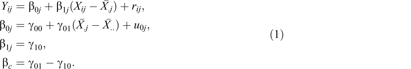
\begin{aligned} Y_{i j} = β_{0 j} + β_{1 j} (X_{i j} - {\overset{ˉ}{X}}_{. j}) + r_{i j}, \\ β_{0 j} = γ_{00} + γ_{01} ({\overset{ˉ}{X}}_{. j} - {\overset{ˉ}{X}}_{. .}) + u_{0 j}, \\ β_{1 j} = γ_{10}, \\ β_{c} = γ_{01} - γ_{10} . \end{aligned}

In Equation 1, Y_ij and X_ij denote the outcome and predictor values of individual i in Level-2 unit j, respectively. For the Level-1 equation, the predictor values are centered on the group means ${\overset{ˉ}{X}}_{. j}$ . For the Level-2 model, the predictor values are centered on the grand mean ${\overset{ˉ}{X}}_{. .}$ .

In typical educational research settings, Y_ij and X_ij can be constructed by summing or averaging item scores from self-reports or other instruments. The random effects r_ij and u _0j are assumed to be normally distributed with zero means and variances σ² and τ₀₀, respectively. In this particular definition of a contextual effect as a compositional effect, the slope $γ_{10}$ is the same across the Level-2 units (a fixed effect).

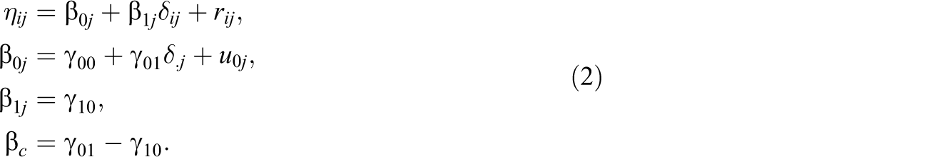
In a nonlinear multilevel latent variable model, the predictors and outcomes become latent variables that are denoted as η _ij and ξ _ij . Those latent variables are connected to manifest variables through measurement models. For notational simplicity, latent individual deviations from latent group means can be defined as $δ_{i j} = ξ_{i j} - ξ_{. j}$ , and group mean deviations from the latent grand mean can be defined as $δ_{. j} = ξ_{. j} - ξ_{. .}$ . Then the latent variable counterpart to Equation 1 is as follows:

\begin{aligned} η_{i j} = β_{0 j} + β_{1 j} δ_{i j} + r_{i j}, \\ β_{0 j} = γ_{00} + γ_{01} δ_{. j} + u_{0 j}, \\ β_{1 j} = γ_{10}, \\ β_{c} = γ_{01} - γ_{10} . \end{aligned}

In Equation 1, η _ij and δ _ij denote the latent outcome and group-centered predictor values of individual i in Level-2 unit j, respectively. At the group level, β_0j is regressed on grand-mean-centered latent group mean $δ_{. j}$ . Note that we have centered the latent Level-1 predictor values around the group means, and the latent Level-2 predictor values around the grant mean, maintaining comparability with Equation 1. Similarly, the random effects r_ij and u _0j are assumed to be normally distributed with zero means and variances σ² and τ₀₀, respectively.

For identification purposes, we impose the restriction of $ξ_{. .} = 0$ to fix the location of the predictor latent variable in the model. This implies that $δ_{. j} = ξ_{. j}$ , and the Level-1 latent predictor value is expressed as a group mean plus a deviation term $ξ_{i j} = ξ_{. j} + δ_{i j}$ . To identify the location of the outcome latent variable, we set the intercept γ₀₀ to zero as well. To identify the scale of the latent variables, we impose additional restrictions on δ _ij and r_ij . These are disturbance terms, so they should have zero means and as is customary in other IRT modeling situations, we set their variances to unity, that is, var(δ _ij ) = 1 and σ² = 1. This particular identification constraint leaves open the possibility to estimate the variance of $ξ_{. j}$ , which will be denoted ψ, as well as the variance of u _0j, which is τ₀₀. We also make the regression model specification assumption that the deviation $ξ_{. j}$ and the random effect u _0j are statistically independent.

2.2 Measurement Models

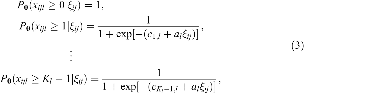
The measurement models define the relationship between manifest variables and latent variables. For brevity, only the measurement models of the latent predictor variable ξ _ij are described in this section, since the measurement models for the latent outcome η _ij can be defined analogously.

When manifest variables are ordinal response variables with multiple categories (including 0 and 1 responses), as is often the case with instruments used in educational research, a logistic version of Samejima’s (1969) classical graded response model can be utilized. Let item l have K_l -ordered categories and $x_{l i j} \in {0, 1, 2, \dots, K_{l} - 1}$ be an element of ith individual’s response in jth group to lth item. The conditional cumulative probability for a response in category $k \in {0, 1, \dots, K_{l} - 1}$ and above are defined as follows:

\begin{aligned} P_{θ} (x_{i j l} \geq 0 | ξ_{i j}) = 1, \\ P_{θ} (x_{i j l} \geq 1 | ξ_{i j}) = \frac{1}{1 + exp [- (c_{1, l} + a_{l} ξ_{i j})]}, \\ ⋮ \\ P_{θ} (x_{i j l} \geq K_{l} - 1 | ξ_{i j}) = \frac{1}{1 + exp [- (c_{K_{l} - 1, l} + a_{l} ξ_{i j})]}, \end{aligned}

where $c_{1, l}, \dots, c_{K_{l} - 1, l}$ represent a vector of K_l − 1 item intercept parameters and a_l is the item slope. The category response probability is defined as the difference between two adjacent cumulative probabilities:

P_{θ} (x_{i j l} = k | ξ_{i j}) = P_{θ} (x_{i j l} \geq k | ξ_{i j}) - P_{θ} (x_{i j l} \geq k + 1 | ξ_{i j}),

for $k \in {0, 1, . . ., K_{l} - 1}$ , where $P_{θ} (x_{i j l} \geq k | ξ_{i j}) = 0$ .

Conditional on ξ _ij , the distribution of x_ijl is multinomial with trial size one in K_l categories:

f_{θ} (x_{i j l} | ξ_{i j}) = \prod_{k = 0}^{K_{l} - 1} P_{θ} (x_{i j l} = k | ξ_{i j})^{χ_{k} (x_{i j l})},

where $χ_{k} (x_{i j l})$ is an indicator function which equals one if and only if x_ijl is equal to k, and 0 otherwise. Note that missing at random observations are handled naturally in this conditional multinomial formulation. The problem of missing not at random observations still remains. If x_ijl is a missing data point, the indicator function is always 0, and hence only observed responses contribute to the measurement of ξ _ij .

The conditional density $f_{θ} (x_{i j l} | ξ_{i j})$ is indexed by θ, which is our generic notation for a vector of all free parameters in the model that includes the item intercepts and slopes, the fixed effects (γ₀₁, γ₁₀), and the variance components (τ₀₀ and ψ). Let $x_{i j} = (x_{i j 1}, \dots, x_{i j L_{x}})^{'}$ be a L_x × 1 vector of item responses from individual i in Level-2 unit j to the L_x items measuring ξ _ij . Invoking the critically important assumption of conditional independence of item responses given the latent variable, we may write

f_{θ} (x_{i j} | ξ_{i j}) = \prod_{l = 1}^{L_{x}} f_{θ} (x_{i j l} | ξ_{i j}) = f_{θ} (x_{i j} | ξ_{. j}, δ_{i j}),

where the last equality follows from the fact that $ξ_{i j} = ξ_{. j} + δ_{i j}$ .

2.3 Observed and Complete Data Likelihoods

Similar to the case of ξ _ij , let us consider the measurement of η _ij . Let L_y be the number of manifest variables for η _ij . Again under conditional independence, the conditional response probabilities factor into item response probabilities:

f_{θ} (y_{i j} | η_{i j}) = \prod_{l = 1}^{L_{y}} f_{θ} (y_{i j l} | η_{i j}),

where y _ij is the L_y × 1 vector of item responses from individual i in Level-2 unit j to the outcome measures. Recall from Equation 2 that

η_{i j} = β_{0 j} + β_{1 j} δ_{i j} + r_{i j} = γ_{00} + γ_{01} ξ_{. j} + u_{0 j} + γ_{10} δ_{i j} + r_{i j} .

We note that given fixed effects, if we knew the random effect $u_{0 j}$ , the latent group mean $ξ_{. j}$ , the latent deviation term $δ_{i j}$ , and the equation disturbance term r_ij , $η_{i j}$ would be completely determined. This implies that we may rewrite the conditional distribution of y _ij as

f_{θ} (y_{i j} | η_{i j}) = f_{θ} (y_{i j} | ξ_{. j}, u_{0 j}, δ_{i j}, r_{i j}) .

If we integrate r_ij out of Equation 8, we have left

f_{θ} (y_{i j} | ξ_{. j}, u_{0 j}, δ_{i j}) = \int f_{θ} (y_{i j} | ξ_{. j}, u_{0 j}, δ_{i j}, r_{i j}) f (r_{i j}) d (r_{i j}),

where f(r_ij ) is the density of a standard normal random variable, given preceding assumptions about the disturbance term. Bringing in results from Equation 6 and integrating out δ _ij yields a conditional density that depends only on the Level-2 latent variables and random effects:

f_{θ} (y_{i j}, x_{i j} | ξ_{. j}, u_{0 j}) = \int f_{θ} (x_{i j} | ξ_{. j}, δ_{i j}) f_{θ} (y_{i j} | ξ_{. j}, u_{0 j}, δ_{i j}) f (δ_{i j}) d (δ_{i j}),

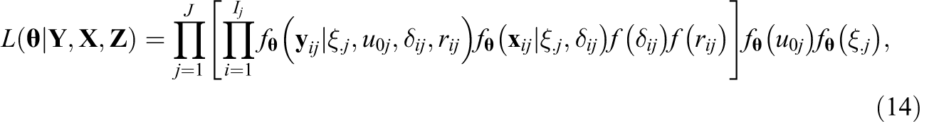
where f(δ _ij ) is the density of a standard normal random variable. Equation 10 makes it clear that we assume, under correct model specification, the outcome measures (y _ij ) and predictor measures (x _ij ) are conditionally independent.

Let J and I_j stand for the number of Level-2 units and number of individuals in Level-2 unit j. Let $Y_{j} = {y_{i j}}_{i = 1}^{I_{j}}$ and $X_{j} = {\{x_{i j}\}}_{i = 1}^{I_{j}}$ represent the collected responses to the outcome manifest variables and predictor manifest variables, respectively, from all individuals in Level-2 unit j. We now make the critical assumption of conditional independence again—that the individuals are independent conditionally on the Level-2 latent variables/random effects $ξ_{. j}$ and u _0j. Thus, the conditional joint density of Y _j and X _j becomes

f_{θ} (Y_{j}, X_{j} | ξ_{. j}, u_{0 j}) = \prod_{i = 1}^{I_{j}} f_{θ} (y_{i j}, x_{i j} | ξ_{. j}, u_{0 j}) .

Integrating out the Level 2 latent variables and random effects yields the marginal probability, wherein we have utilized the independence of $ξ_{. j}$ and u _0j:

f_{θ} (Y_{j}, X_{j}) = \int \int \prod_{i = 1}^{I_{j}} f_{θ} (Y_{j}, X_{j} | ξ_{. j}, u_{0 j}) f (ξ_{. j}) f (u_{0 j}) d (ξ_{. j}) d (u_{0 j}) .

By this point, we have integrated all latent variables and random effects out of the joint probabilities. We now make the routine multilevel modeling assumption that the Level-2 units are the independent sampling units. Upon observing Y _j and X _j and treating them as fixed, the marginal (observed data) likelihood function for the entire sample is as follows:

L (θ | Y, X) = \prod_{j = 1}^{J} f_{θ} (Y_{j}, X_{j}),

where $Y = {\{Y_{j}\}}_{j = 1}^{J}$ and $X = {\{X_{j}\}}_{j = 1}^{J}$ collect together the full set of outcome and predictor observed variable responses, respectively. Directly maximizing this marginal likelihood function over θ would lead to the maximum marginal likelihood estimator of the structural parameters.

An obvious computational limitation to the direct marginal likelihood approach is the integration involved in arriving at the observed data likelihood. All of the integrals must be approximated numerically, which can be computationally challenging. An alternative stance is to treat the random effects and latent variables r_ij , δ _ij , $ξ_{. j}$ , and u _0j as missing data. This leads to a missing data formulation of the latent variable model. Had the missing data been observed, the complete data likelihood function can be written as

L (θ | Y, X, Z) = \prod_{j = 1}^{J} [\prod_{i = 1}^{I_{j}} f_{θ} (y_{i j} | ξ_{. j}, u_{0 j}, δ_{i j}, r_{i j}) f_{θ} (x_{i j} | ξ_{. j}, δ_{i j}) f (δ_{i j}) f (r_{i j})] f_{θ} (u_{0 j}) f_{θ} (ξ_{. j}),

where Z collects together all the Level-1 random effects/latent variables ${\{{r_{i j}, δ_{i j}}_{i = 1}^{I_{j}}\}}_{j = 1}^{J}$ as well as those at Level-2 ${\{u_{0 j}, ξ_{. j}\}}_{j = 1}^{J}$ . In other words, Z represents the “missing data.”

This missing data formulation prompts us to consider an alternative estimation approach that eschews numerical integration. In particular, the missing data may be “filled in” by drawing imputations from their posterior predictive distribution $f (Z | Y, X, θ)$ . Note that in our case the posterior predictive distribution is proportional to the complete data likelihood, greatly facilitating the use of MCMC sampling methods to draw from the posterior. The imputations lead to complete data sets, and the complete data likelihood function is much easier to handle than the observed data likelihood function due to its completely factored form. Instead of directly solving the observed data optimization problem, a sequence of complete data optimizations can iteratively improve the parameters estimates until convergence.

3 MH-RM Algorithm for Contextual Models

3.1 MH-RM Algorithm

The MH-RM algorithm was initially proposed by Cai (2008) for nonlinear latent structure analysis with a comprehensive measurement model, and the application of the algorithm has been expanded to other measurement and statistical models (e.g., Cai, 2010a, 2010b; Monroe & Cai, 2014). The MH-RM algorithm is an extension of the Stochastic Approximation EM algorithm (Celeux, Chauveau, & Diebolt, 1995; Celeux & Diebolt, 1991; Delyon, Lavielle, & Moulines, 1999). The MH-RM algorithm combines the Metropolis–Hastings (MH; Hastings, 1970; Metropolis, Rosenbluth, Rosenbluth, Teller, & Teller, 1953) algorithm and the Robbins–Monro (RM; Robbins & Monro, 1951) stochastic approximation algorithm.

Utilizing the missing data formation of the latent variable model, the random effects and latent variables are treated as missing data (e.g., Gu & Kong, 1998). Once the missing data are “filled in” by the MH sampler, complete data likelihoods can be optimized iteratively. Because imputation noise is introduced in the MH step, the RM algorithm is used to filter out the noise. Let the parameter estimate at iteration t be denoted $θ^{(t)}$ , the (t + 1)th iteration of the MH-RM algorithm consists of three steps: Stochastic Imputation, Stochastic Approximation, and Robbins–Monro Update.

Step 1: Stochastic Imputation

Draw M_t sets of missing data, which are the random effects and the latent variables, from a Markov chain that has the posterior predictive distribution of missing data $f (Z | Y, X, θ^{(t)})$ as the target. Then, M_t sets of complete data are formed as follows:

\{Y, X, Z_{m}^{(t + 1)}; m = 1, . . ., M_{t}\} .

Step 2: Stochastic Approximation

Let

s (θ^{(t)} | Y, X, Z_{m}^{(t + 1)}) = \frac{\partial}{\partial θ} log L (θ^{(t)} | Y, X, Z_{m}^{(t + 1)})

denote the gradient vector of the complete data log-likelihood function, evaluated at the current parameter value θ^(t) and missing data imputation $Z_{m}^{(t + 1)}$ . We first compute the sample average of gradients of the complete data log likelihood:

{\tilde{s}}_{t + 1} = \frac{1}{m_{t}} \sum_{m = 1}^{M_{t}} s (θ^{(t)} | Y, X, Z_{m}^{(t + 1)}) .

By Fisher’s (1925) Identity, the conditional expectation of the complete data gradient vector over the posterior distribution of the missing data is the same as the gradient vector of the observed data log likelihood, under mild regularity conditions; that is,

\frac{\partial}{\partial θ} log L (θ | Y, X) = \int \frac{\partial}{\partial θ} log L (θ | Y, X, Z) f (Z | Y, X, θ) d Z .

In other words, though noise corrupted, ${\tilde{s}}_{t + 1}$ gives the direction of likelihood ascent because it is a Monte Carlo approximation of the conditional expected complete data gradient vector (the right-hand side of Equation 18), which is also an approximation of the observed data gradient vector (the left-hand side of Equation 18).

Step 3: Robbins–Monro Update

To improve stability and speed, we also compute $Γ_{t + 1}$ which is a recursive approximation of the conditional expectation of the information matrix of the complete data log likelihood at (t + 1)th iteration (e.g., Cai, 2008; Gu & Kong, 1998):

Γ_{t + 1} = Γ_{t} + ε_{t} [\frac{1}{M_{t}} \sum_{m = 1}^{M_{t}} H (θ^{(t)} | Y, X, Z_{m}^{(t + 1)}) - Γ_{t}],

where

H (θ | Y, X, Z) = - \frac{\partial^{2}}{\partial θ \partial θ^{'}} log L (θ | Y, X, Z),

is the complete data information matrix, that is, the negative second derivative matrix of the complete data log likelihood. Updated parameters are computed recursively:

θ^{(t + 1)} = θ^{(t)} + ε_{t} (Γ_{t + 1}^{- 1} {\tilde{s}}_{t + 1}),

where ${ε_{t}; t \geq 0}$ is a sequence of gain constants.

The gain constant ε _t is a sequence of decreasing nonnegative real numbers such that $ε_{t} \in (0, 1]$ , $\sum_{t = 0}^{\infty} ε_{t} = \infty$ , and $\sum_{t = 0}^{\infty} ε_{t}^{2} < \infty$ . In practical implementations of MH-RM, the starting parameter values θ⁽⁰⁾ are often sufficiently far away from the mode of the marginal likelihood that extra care must be taken with the gain constant sequence so that MH-RM does not terminate prematurely. We typically implement a three-stage procedure wherein the first M1 iterations of MH-RM use nondecreasing gain constants to quickly move the provisional estimates to a vicinity of the final solution. The next M2 iterations use the same nondecreasing gain constants, but the estimates are averaged to start the final MH-RM iterations with decreasing gain constants. For the last stage, the sequence of gain constants is taken to be $ε_{t} = 0.1 / (t + 1)^{0.75}$ after experiments that monitor the traces of parameters using simulated data sets.

The iterations are started from initial values θ⁽⁰⁾ and a positive definite matrix $Γ_{0}$ . For this study, estimates from traditional HLM analysis were used for initial values and corresponding $Γ_{0}$ .

They can be terminated when the changes in parameter estimates are sufficiently small. As a practical method for convergence check, Cai (2008) proposed to monitor a “window” of the largest absolute differences between two adjacent iterations. Cai suggested three as a reasonable width of the window to be monitored in practice. Cai showed that the MH-RM iterations converge to a local maximum of the observed data likelihood $L (θ | Y, X)$ with probability one as t increases without bounds.

3.2 Approximating the Observed Information Matrix

One of the benefits of using the MH-RM algorithm is that the observed data information matrix can be approximated as a by-product of the iterations. The inverse of the observed data information matrix becomes the large-sample covariance matrix of parameter estimates. The square root of the diagonal elements are the standard errors (SEs). Utilizing Fisher’s Identity, the gradient vector is approximated recursively,

{\hat{s}}_{t + 1} = {\hat{s}}_{t} + ε_{t} {{\tilde{s}}_{t + 1} - {\hat{s}}_{t}},

where ${\tilde{s}}_{t}$ is defined as in Equation 17. A Monte Carlo estimate of the conditional expectation of the complete data information matrix minus the conditional covariance of the complete data gradient vector is defined as follows:

{\tilde{G}}_{t} = \frac{1}{M_{t}} \sum_{m = 1}^{m_{t}} \{H (θ^{(t)} | Y, X, Z_{m}^{(t + 1)}) - s (θ^{(t)} | Y, X, Z_{m}^{(t + 1)}) {[s (θ^{(t)} | Y, X, Z_{m}^{(t + 1)})]}^{'}\} .

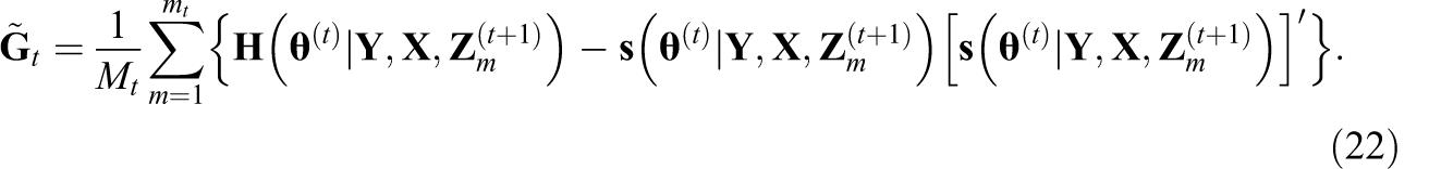
A more stable estimate can be found by further recursive approximation:

{\hat{G}}_{t + 1} = {\hat{G}}_{t} + ε_{t} \{{\tilde{G}}_{t + 1} - {\hat{G}}_{t}\} .

Finally, the observed information matrix is approximated as follows:

I_{t + 1} = {\hat{G}}_{t + 1} + {\hat{s}}_{t + 1} {\hat{s^{'}}}_{t + 1} .

Gu and Kong (1998) and Cai (2010a) discussed the rationale behind this approximation as a recursive application of Louis’s (1982) formula. The main benefit is that the information matrix becomes a by-product of the MH-RM iterations. Another practical option for approximating the observed information matrix is a direct application of Louis’s (1982) formula, in which additional Monte Carlo samples are used after convergence to directly approximate the gradient vector and the conditional expectations. In this study, SEs obtained by the first method are called recursively approximated standard errors and those from the latter are called post-convergence approximated standard errors. The reader should, however, keep in mind that the likelihood surface of nonlinear multilevel models such as this one may be irregular and inference using curvature information provided by second derivatives should always be taken with a grain of salt.

4 Simulation Studies

4.1 Simulation Study 1: Comparison of Estimation Algorithms

4.1.1 Methods

The first study examined parameter recovery and SEs across two algorithms, an MH-RM algorithm and an existing EM algorithm. The data generating and fitted models followed Equation 2. The simulated data are balanced in that the number of Level-2 units (ng) is 100 and the number of Level-1 units per group (np) is 20. The generating ICC value for the latent predictor was 0.3.

For the measurement model, five dichotomously scored manifest variables were generated for each latent trait (i.e., η and ξ) using the graded response model in Equation 3. For η _ij , the manifest variables are $Y_{1}, Y_{2}, Y_{3}, Y_{4},$ and $Y_{5}$ . For ξ _ij , which is the sum the Level-2 latent group mean and the deviation terms ( $ξ_{. j} + δ_{i j}$ ), the manifest variables are X ₁, X ₂, X ₃, X ₄, and X ₅. The item parameters were the same across levels, representing cross-level measurement invariance.

We attempted 100 Monte Carlo replications. The first 10 data sets were analyzed using two methods: an MH-RM algorithm implemented in R (R Core Team, 2012) and an adaptive quadrature-based EM approach implemented in Mplus (L. K. Muthén & Muthén, 2010). The MH-RM algorithm’s convergence criterion was 5.0 × 10⁻⁵, and the maximum number of iterations for the first two stages of MH-RM with constant gains were M1 = 100 and M2 = 500. To calculate post-convergence approximated SEs, 100 to 500 additional random samples were used. All replications converged within 600 MH-RM iterations with decreasing gains.

4.1.2 Results

The generating values and the corresponding estimates for the compositional effect from different algorithms are summarized in Table 1. The first column contains the true parameters for the measurement and structural parameters. The second set of columns and the third set of columns include the estimates and SEs from EM with different numbers of adaptive quadrature points (qp = 5 and qp = 14). The default number of quadrature points is 15 in Mplus, but the computer cannot handle 15 quadrature points for this four-dimensional model. The maximum possible number of quadrature points was 14 for a compositional effect model. A smaller number of quadrature points, five, was tested to compare point estimates and SEs. The fourth set of columns includes the corresponding point estimates and SEs using the MH-RM algorithm.

Table 1

Generating values, EM Estimates, and MH-RM Estimates for a Compositional Effect Model

Structural Parameters
		EM (5 qp)		EM (14 qp)		MH-RM
	θ	E( $\hat{θ}$ )	E{SE( $\hat{θ}$ )}	E( $\hat{θ}$ )	E{SE( $\hat{θ}$ )}	E( $\hat{θ}$ )	E{SE( $\hat{θ}$ )}
γ₀₁	1.00	1.02	.19	1.01	.19	1.00	.18
γ₁₀	0.50	0.52	.05	0.51	.05	0.52	.09
τ₀₀	1.00	0.90	.16	0.91	.17	0.93	.16
ψ	0.43	0.40	.07	0.42	.07	0.42	.07
Measurement Parameters
a_x ₁	0.80	0.79	.07	0.79	.07	0.79	.08
a_x ₂	1.00	1.01	.08	1.01	.08	1.00	.09
a_x ₃	1.20	1.24	.09	1.24	.09	1.24	.11
a_x ₄	1.40	1.39	.10	1.39	.10	1.39	.12
a_x ₅	1.60	1.67	.14	1.67	.14	1.69	.15
a_y ₁	0.80	0.78	.06	0.78	.06	0.78	.06
a_y ₂	1.00	1.00	.07	1.00	.07	1.00	.07
a_y ₃	1.20	1.23	.09	1.23	.09	1.23	.08
a_y ₄	1.40	1.40	.11	1.40	.11	1.40	.10
a_y ₅	1.60	1.61	.13	1.61	.13	1.60	.12
c_x ₁	−0.80	−0.75	.08	−0.75	.08	−0.75	.06
c_x ₂	0.00	0.02	.08	0.02	.08	0.02	.05
c_x ₃	1.20	1.30	.11	1.30	.11	1.29	.08
c_x ₄	−0.70	−0.61	.11	−0.61	.11	−0.62	.07
c_x ₅	0.80	0.92	.14	0.92	.14	0.92	.08
c_y ₁	−0.80	−0.80	.11	−0.80	.11	−0.81	.06
c_y ₂	0.00	0.01	.13	0.01	.13	0.00	.05
c_y ₃	1.20	1.19	.16	1.19	.16	1.18	.08
c_y ₄	−0.70	−0.74	.18	−0.74	.18	−0.75	.07
c_y ₅	0.80	0.79	.21	0.79	.21	0.78	.08
Computational Efficiency
One processor		5˜7 min		60˜100 min		35 ˜ 40 min

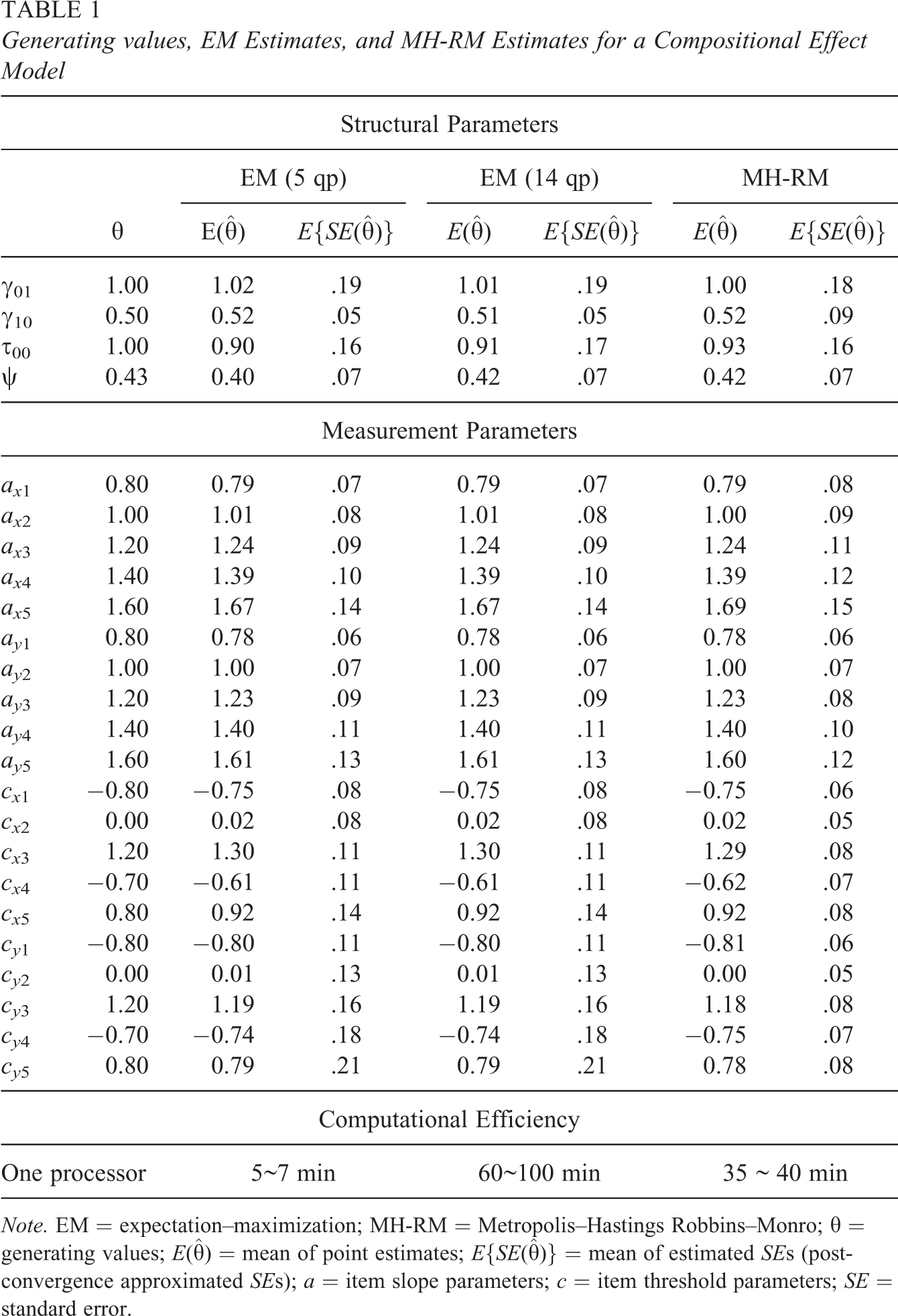
Note. EM = expectation–maximization; MH-RM = Metropolis–Hastings Robbins–Monro; θ = generating values; E( $\hat{θ}$ ) = mean of point estimates; E{SE( $\hat{θ}$ )} = mean of estimated SEs (post-convergence approximated SEs); a = item slope parameters; c = item threshold parameters; SE = standard error.

The means of point estimates from different algorithms are generally very close to one another. For structural parameter estimates, the number of quadrature points does not appear to make a large difference, though 14-quadrature-point estimates are slightly closer to the MH-RM estimates and the generating values in terms of τ₀₀ and ψ. SEs are also very similar.

For measurement parameter estimates, both the means of point estimates and the SEs were the same up to the second decimal place across different numbers of quadrature points. The largest difference in average point estimates between EM and MH-RM was 0.02, indicating that the two approaches yield highly similar estimates. However, mean SE estimates are slightly different between MH-RM and EM results in that the SE estimates from MH-RM algorithm for intercepts are smaller than those from the EM algorithm. The biggest difference in SE estimates for measurement parameters between two algorithms was 0.13.

The natural logarithm of SE estimates from EM algorithm and MH-RM algorithm (post-convergence approximated SEs) are plotted against the natural logarithm of empirical standard deviations of the point estimates across the Monte Carlo replications in Figure 1. The estimates are clustered along the diagonal reference line, indicating that the estimated SEs are generally close to the Monte Carlo standard deviations of the point estimates, except for the intercept parameter SEs, which appear to be underestimated when the post-convergence approximation is used for the MH-RM algorithm.

Figure 1.

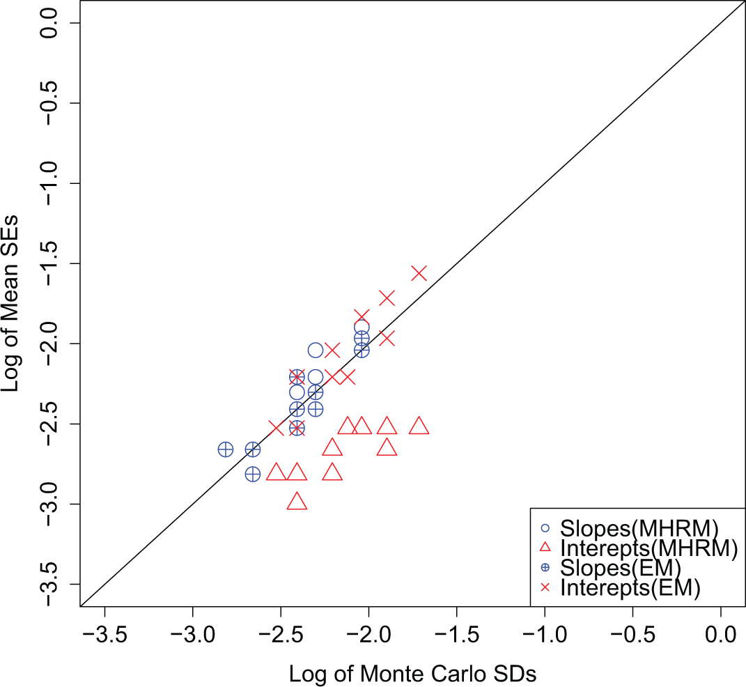
Comparisons of standard errors (SEs) for item parameters.

With regard to computing time, when one processor was used for estimation, EM with 5 quadrature points generally required a small amount of time, while EM with 14 quadrature points generally required over an hour. The MH-RM algorithm required about 40 minutes. Note that MH-RM is implemented in R (an interpreted language) with explicit looping, while Mplus is written in FORTRAN (a compiled language). As an interpreted language is expected to be several orders of magnitude slower compared to a compiled language in terms of looping, a direct comparison is inappropriate. What we can safely conclude is that when ported into a compiled language, MH-RM is poised to be substantially faster.

To examine the performance of the MH-RM algorithm further, all 100 generated data sets were analyzed, and the results are summarized in Table 2. The means of point estimates are reasonably close to generating values in general, with slight underestimation of variance components. The Monte Carlo standard deviations of parameter estimates (column 5) are also similar to SE estimates from both EM and MH-RM (columns 4 and 6); the largest difference is 0.02. With respect to measurement parameters, the average item parameter estimates are very close to generating values.

Table 2

Generating Values and MH-RM Estimates for a Compositional Effect Model

Structural Parameters
	θ	E( $\hat{θ}$ )	E{SE1( $\hat{θ}$ )}	SD( $\hat{θ}$ )	E{SE2( $\hat{θ}$ )}	95% CI Coverage Using SE1
γ₀₁	1.00	0.99	0.17	0.19	0.18	95.0
γ₁₀	0.50	0.50	0.06	0.07	0.09	95.0
τ₀₀	1.00	0.97	0.20	0.18	0.16	89.0
ψ	0.43	0.43	0.08	0.09	0.07	89.0
Measurement Parameters
a_x ₁	0.80	0.80	0.07	0.06	0.07	98.0
a_x ₂	1.00	1.01	0.10	0.09	0.09	91.0
a_x ₃	1.20	1.22	0.12	0.10	0.11	92.0
a_x ₄	1.40	1.40	0.12	0.10	0.13	84.0
a_x ₅	1.60	1.60	0.15	0.13	0.15	73.0
a_y ₁	0.80	0.80	0.07	0.07	0.06	95.0
a_y ₂	1.00	1.01	0.07	0.07	0.07	94.0
a_y ₃	1.20	1.21	0.10	0.09	0.09	86.0
a_y ₄	1.40	1.39	0.10	0.09	0.10	89.0
a_y ₅	1.60	1.61	0.10	0.13	0.13	74.0
c_x ₁	0.80	0.80	0.14	0.08	0.06	94.0
c_x ₂	0.00	0.00	0.07	0.09	0.05	95.0
c_x ₃	−1.20	−1.22	0.09	0.12	0.08	91.0
c_x ₄	0.70	0.69	0.12	0.11	0.07	89.0
c_x ₅	−0.80	−0.80	0.12	0.15	0.08	89.0
c_y ₁	0.80	0.81	0.08	0.09	0.06	87.0
c_y ₂	0.00	0.01	0.11	0.11	0.06	78.0
c_y ₃	−1.20	−1.20	0.13	0.13	0.08	75.0
c_y ₄	0.70	0.71	0.15	0.15	0.07	62.0
c_y ₅	−0.80	−0.79	0.14	0.18	0.08	59.0
Computational Efficiency
			35˜40 min		90˜120 min

Note. MH-RM = Metropolis–Hastings Robbins–Monro; CI = confidential interval; θ = generating values; E( $\hat{θ}$ ) = mean of point estimates; E{SE1( $\hat{θ}$ )} = mean of recursively approximated standard error (SE) estimates; E{SE2( $\hat{θ}$ )} = mean of post-convergence approximated SEs; SD( $\hat{θ}$ ) = Monte Carlo standard deviation of point estimates; 95% confidence interval coverage rate using post-convergence approximated SEs; a = item slope parameters; c = item threshold parameters.

However, we see that recursively approximated SEs are generally closer to the Monte Carlo standard deviations of item parameter estimates than the post-convergence approximated SEs. More specifically, the most prominent differences are found in the SEs of intercept parameters, where post-convergence approximated SEs for item intercept parameters are underestimated. Therefore, we find that recursively approximated SEs perform better than post-convergence approximated SEs. With that said, a drawback of using recursively approximated SEs is the requirement of a relatively larger number of main MH-RM iterations (at least 1,000 in our experience) to reach a positive definite approximate observed information matrix. For this reason, post-convergence approximated SEs are adopted for the remaining simulations in this study since this approach gives proper SE estimates for structural parameters and can be faster.

Finally, 95% confidence intervals for each parameter were calculated. The post-convergence approximated SEs were used to form these two-sided Wald-type confidence intervals. The percentages of intervals that cover the generating values are reported in the last column of Table 2. Based on the 100 replications performed, coverage of structural parameters appears well calibrated in general. For measurement parameters, the coverage rates tend to decrease as the magnitude of parameters becomes larger. Coverage rates are at the lowest for the more extreme intercept parameters due to their underestimated SEs.

4.2 Simulation Study 2: Comparison of Models

The second simulation study was conducted to examine how measurement error and sampling error may influence compositional effect estimation across different conditions with both a traditional HLM and a multilevel latent variable model.

4.2.1 Simulation conditions

A total of 30 data generating conditions were examined: two compositional effect sizes $\times$ three sampling conditions $\times$ two ICC sizes $\times$ two measurement conditions + six conditions for a model with no compositional effect.

First, two different sizes of compositional effect were considered in this study. The generating value of $γ_{01}$ was 1.0. The generating value of $γ_{10}$ was either 0.5 or 0.8, giving a compositional effect of 0.5 or 0.2, respectively. Second, the combination of large (ng = 100, np = 20) and small (ng = 25, np = 5) numbers of groups and individuals makes a total of four different sampling conditions. However, the combination of 25 groups and group size of 5 leads to too small a total sample size (125), which is not entirely appropriate for the stable estimation of a high-dimensional latent variable model. Therefore, only three different sampling conditions were used for this simulation study. For latent predictor ICC levels, 0.1 and 0.3 were used to generate small- and large-ICC conditions by manipulating ψ, the variance of $ξ_{. j}$ . Finally, two different measurement structures were considered. The observed variables in the first condition were dichotomous and in the second condition, they were five-category ordinal responses. The true item parameters are given in Appendix Table A1. Additionally, data were generated from a model with no compositional effect ( $γ_{01} = γ_{10}$ ) with the first measurement condition and analyzed to examine empirical Type I error rates for the compositional effect estimates with both the traditional model and the latent variable model. In each condition, 100 Monte Carlo replications were attempted.

4.2.2 Analysis

Because all simulated data sets have the true generating values of η _ij and ξ _ij , these values (true scores) can be analyzed using a traditional model. The resulting parameter estimates can be considered gold standard estimates that are influenced only by sampling fluctuations but not by measurement conditions. Therefore, each data set has three sets of parameter estimates: (1) estimates from analyzing the generating values of η _ij and ξ _ij with a traditional HLM, which is treated as the gold standard, (2) estimates obtained by applying the latent variable model, and (3) the estimates from analyzing the observed summed scores of outcomes and predictors with the standard approach using manifest variables. All of the traditional HLM analyses were conducted using an R package nlme (Pinheiro, Bates, DebRoy, Sarkar, & R Core Team, 2012).

4.2.3 Evaluation statistics

To compare these three sets of estimates, the following three statistics are calculated: (1) the percentage bias of the estimate relative to the magnitude of its generating value, (2) the observed coverage rate of the 95% confident interval, and (3) the observed power to detect the compositional effect of interest as significant.

It should be noted that the regression coefficient estimates from the observed sum score analysis using a traditional multilevel model are not on the same scales as those obtained using the latent variable approach, which yields naturally standardized fixed effects coefficients due to the identification conditions discussed earlier. To make the coefficient estimates more comparable, the estimates from the traditional HLM approach were standardized by multiplying the parameter estimates by the ratio of standard deviation of the predictor to the standard deviation of the outcome.

4.2.4 Results

Convergence rates and mean computing time across generating data conditions are reported in Appendix Table A2. Only converged replications were used to calculate evaluation statistics. In general, the convergence rates at fixed number of iterations (M1 = 100 and M2 = 500) are over 90%. The worst cases of nonconvergence occur when the number of Level-2 units is low and the ICC is small (roughly 80%). The nonconvergence occurs for the approximation of observed information matrix that should be a positive definite. This is particularly true for the second measurement condition when a substantially larger number of item parameters for the multiple-categorical items must be estimated from the data. While more iterations could increase the convergence rates, the nonconvergence rates for the combination of small ICC and small cluster size are informative in that converged solutions might not be available for more extreme conditions.

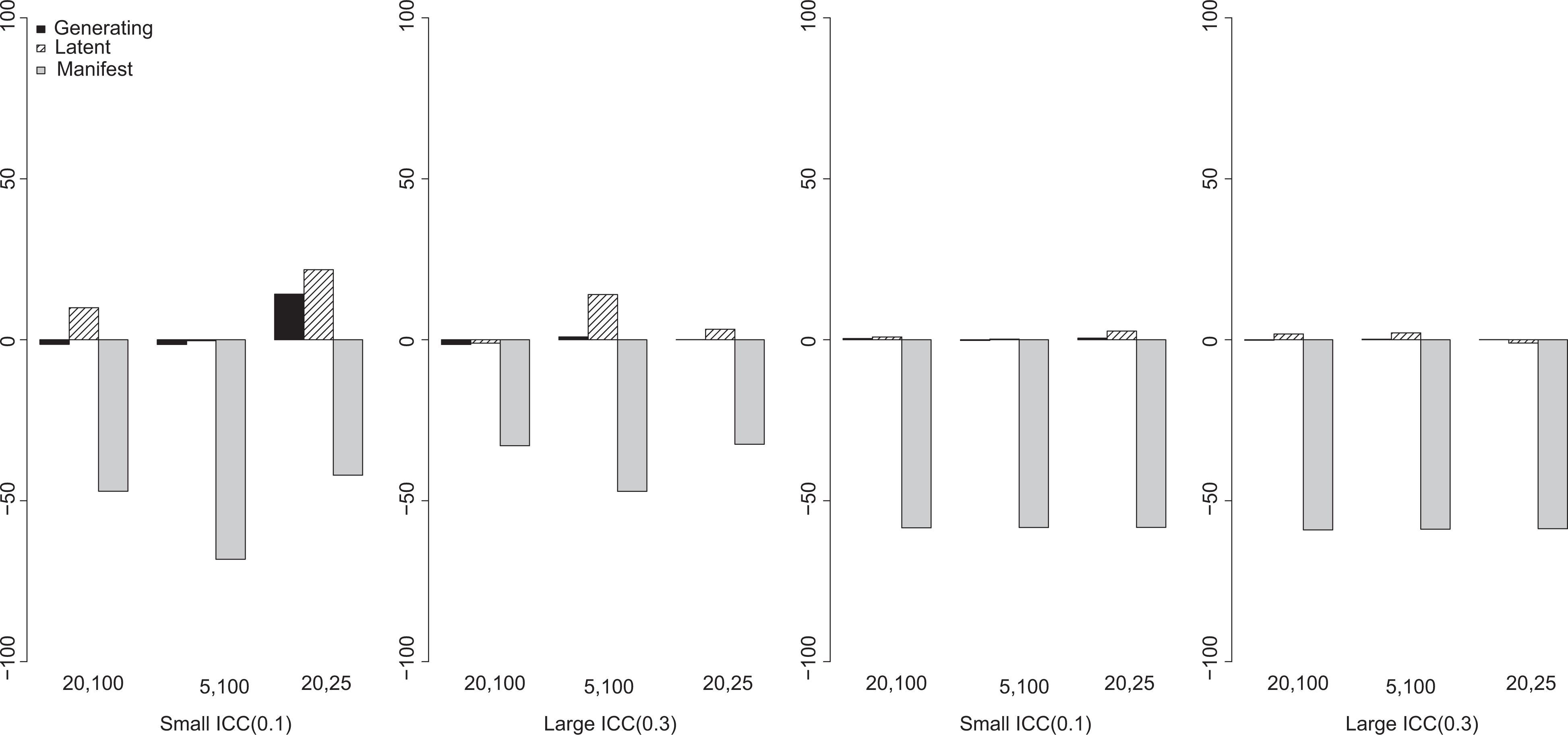
Let us examine the first measurement condition where all items are dichotomously scored. Because a compositional effect estimate is defined as the difference between ${\hat{γ}}_{01}$ and ${\hat{γ}}_{10}$ , those two parameter estimates are examined together, along with the compositional effect estimate itself (the difference). Relative percentage biases in ${\hat{γ}}_{01}$ and ${\hat{γ}}_{10}$ are summarized in Figure 2. When the generating values of η _ij and ξ _ij were analyzed, the bias of ${\hat{γ}}_{01}$ ranged from 1% to 15% across the sampling conditions. Latent variable modeling resulted in a similar magnitude of bias. But traditional HLM resulted in more substantial bias in both ${\hat{γ}}_{01}$ and ${\hat{γ}}_{10}$ (from 30% to 70%; see the gray bars in Figure 2).

Figure 2.

Relative percentage bias in ${\hat{γ}}_{01}$ (first two plots) and ${\hat{γ}}_{10}$ (last two plots), large true compositional effect, measurement condition 1, by the sampling conditions (number of individuals in each group and number of groups).

The biases in the traditional HLM estimates of the regression coefficients lead to an interesting pattern of biases in the compositional effect estimate. The bias can be as small as 8% when the predictor ICC is large and the sampling condition favorable (more individuals in each group), but the bias can be as large as 80% when the ICC is small and the group size is small (see Figure 3). It is also noteworthy that the bias in the compositional effect estimate from the traditional HLM model can also be positive when the ICC is large and the contextual effect size is small (see the last plot of Figure 3).

Figure 3.

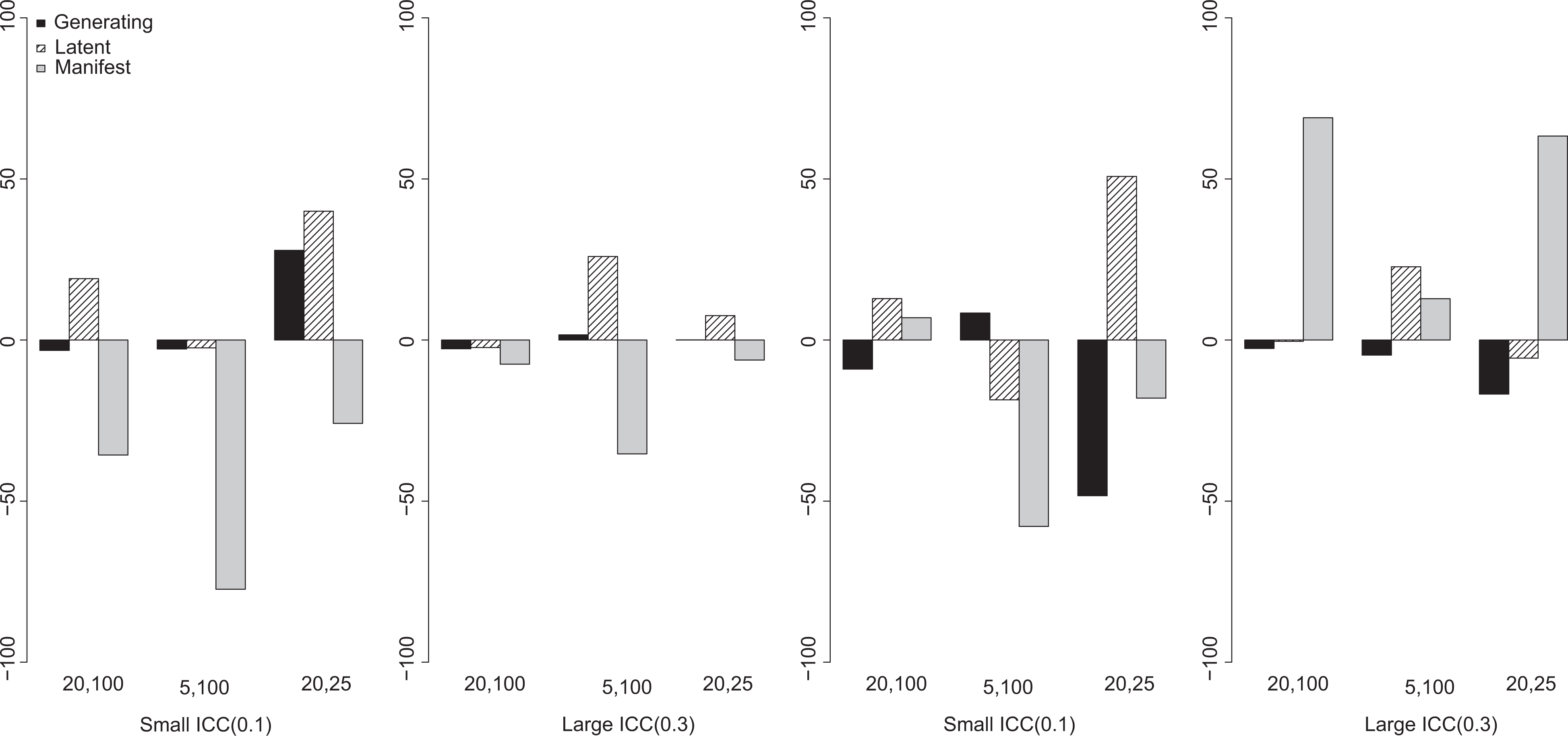
Relative percentage bias in compositional effect estimate ${\hat{γ}}_{01} - {\hat{γ}}_{10}$ , large true compositional effect (first two plots) and small true compositional effect (last two plots), first measurement condition, by the sampling conditions (number of individuals in each group and number of groups).

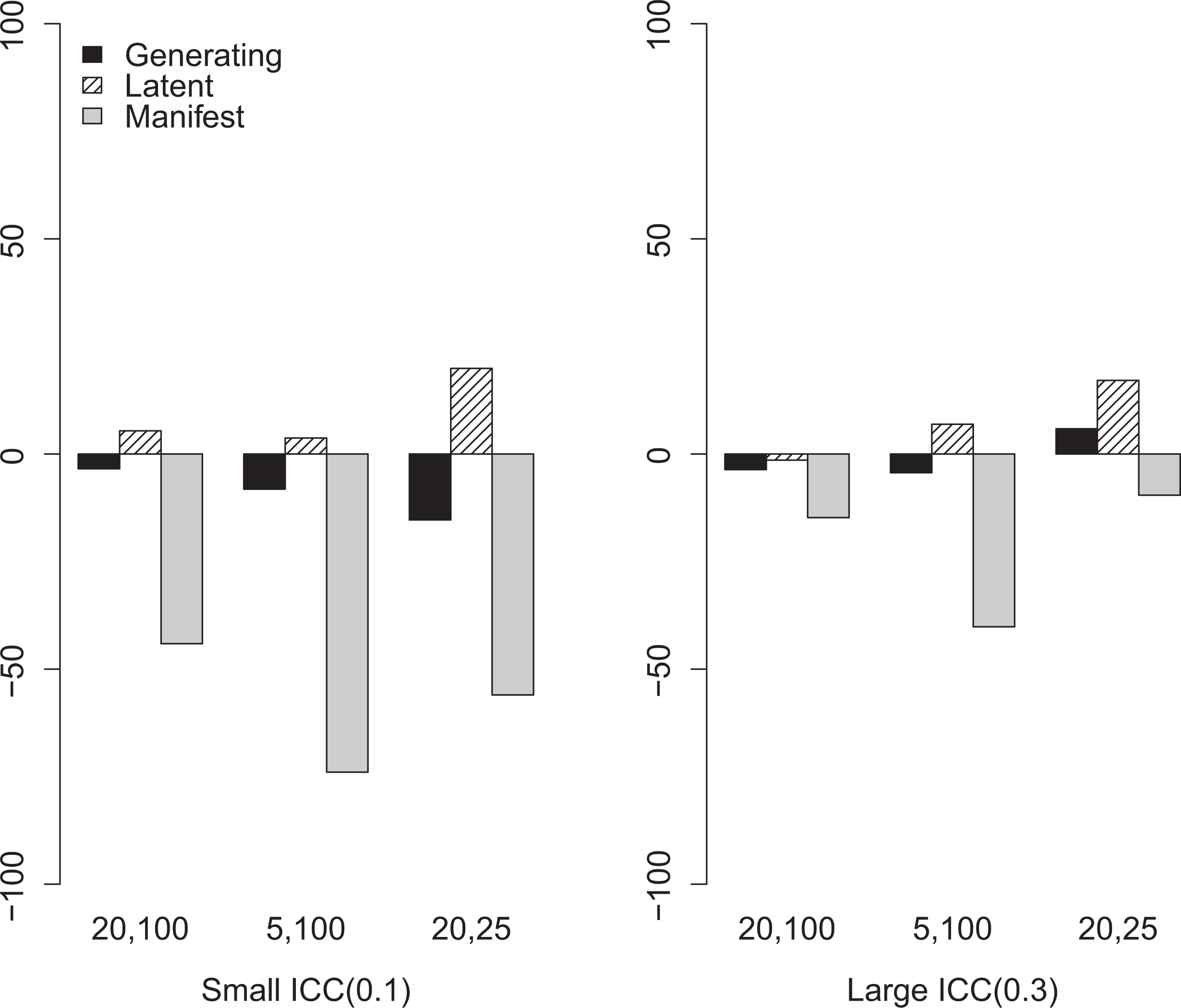
On the other hand, comparing the two plots in Figure 4 with the first two plots in Figure 3 reveals that the performance of the traditional HLM and the latent variable model in terms of estimating ${\hat{γ}}_{01}$ , ${\hat{γ}}_{10}$ , as well as the compositional effect, is highly similar across the two measurement conditions. This indicates the measurement model is a less influential source of bias in this study.

Figure 4.

Relative percentage bias in compositional effect estimate ${\hat{γ}}_{01} - {\hat{γ}}_{10}$ , large true compositional effect, second measurement condition, by the sampling conditions (number of individuals in each group and number of groups).

To examine the SE estimates, the coverage rates of the 95% confidence intervals for the true compositional effect were calculated. Results from the condition with large true compositional effect and the first measurement condition are summarized in Figure 5. When generating values are analyzed, the coverage rates across sampling conditions are generally close to 95%, except for the case where the ICC is small and the number of groups is also small. In this case, the coverage rate can be as low as 85%. The coverage rates based on the latent variable model parameter estimates were similar or slightly worse than those from generating value analysis. Coverage rates with traditional HLM estimates can be problematic when both the number of individuals per group and the ICC are low.

Figure 5.

Niney-five percent compositional effect estimate confidence interval coverage rates, large true compositional effect, first measurement condition, by the sampling conditions (number of individuals in each group and number of groups).

To examine how researchers can make different inferential decisions when they apply a traditional model and a latent variable model, the empirical Type I error rates are calculated for the conditions where the true data generating model has zero compositional effect. Figure 6 shows empirical Type I error rates across the ICC and sampling conditions for the first measurement condition.

Figure 6.

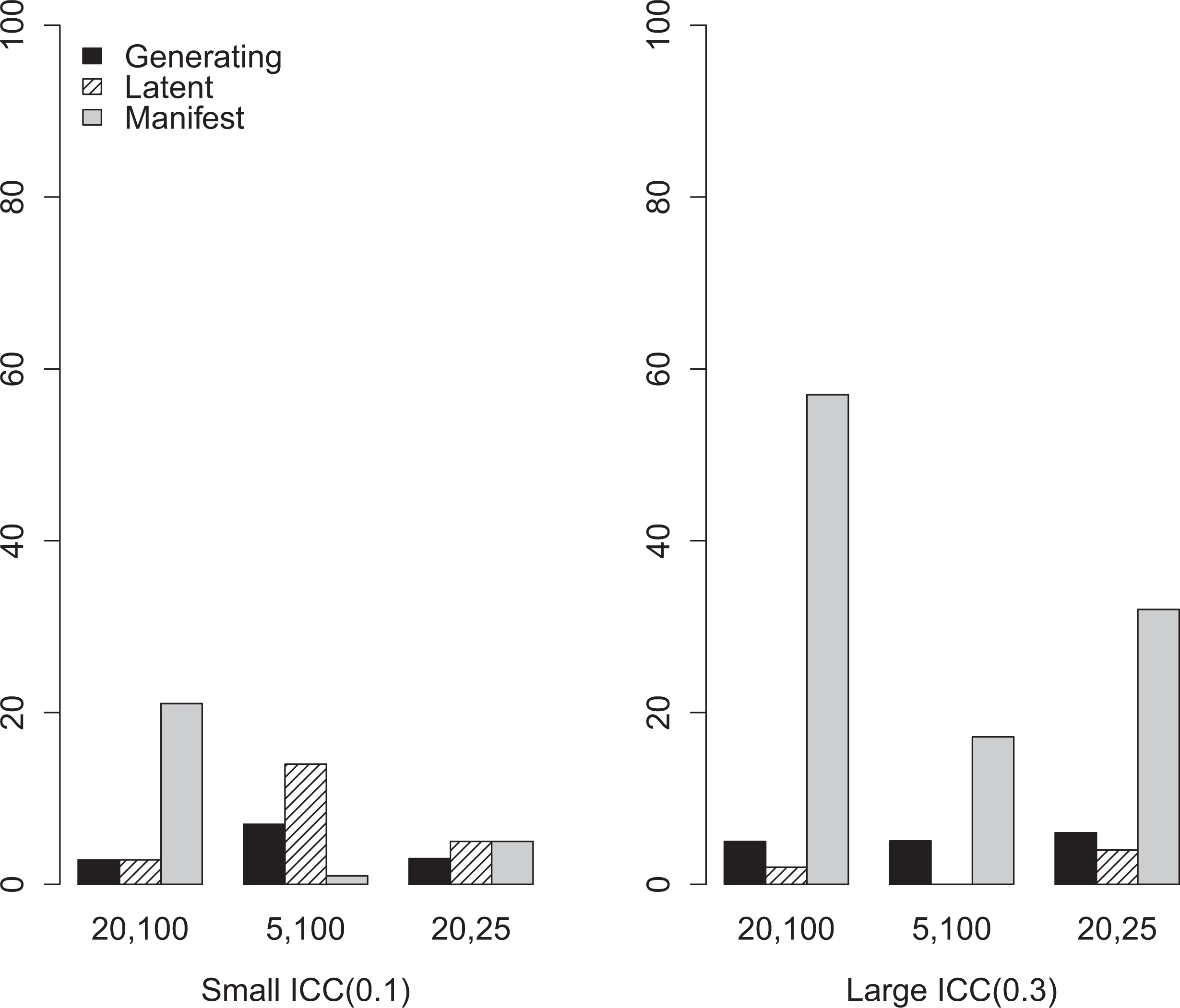
Empirical Type I error rates for the compositional effect estimate, first measurement condition.

Generating value analysis yields Type I error rates of .05 to .07 across sampling conditions. The latent variable model maintains similar Type I error rate calibration, except for the cases when the number of individuals per group is small. For traditional HLM analysis, Type I error rate inflation is dramatic. Only under the conditions when a small predictor ICC is coupled with a small number of group or a small number of individuals per group, does the traditional method maintains proper Type I error rate.

Turning to statistical power, when a compositional effect is large (see Figure 7), generating value analysis yields power of about .85 when the ICC is large and the number of groups is also large. When the ICC is small, power decreases to .35 even with favorable sampling conditions. The lowest statistical power (.15) is found when predictor ICC is small and the number of groups is also small.

Figure 7.

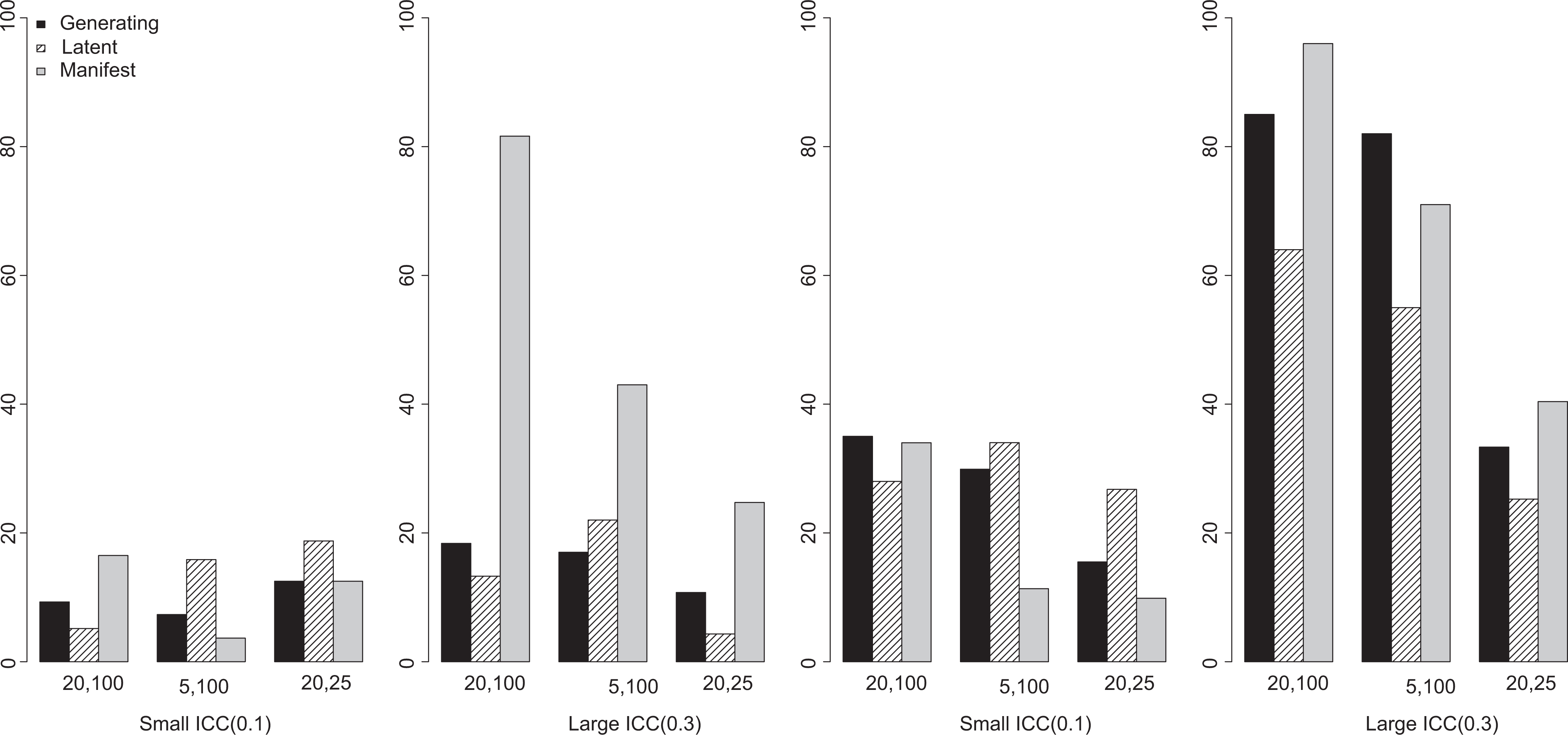
Percentage of significant compositional effect (estimated power), small true compositional effect (first two plots), and large true compositional effect (last two plots), first measurement condition.

The patterns are similar for the latent variable analysis. But when ICC is small, and the number of individuals per group or the number of groups is small, latent variable modeling actually yields a slightly higher percentage of significant compositional effects. While the traditional HLM analysis yields a very high percentage of significant compositional effects when the ICC is large and the number of individuals per group is also large, the power decreases remarkably when the ICC is small and when the sampling condition deteriorates (i.e., when the number of individuals per group or the number of groups is small). Also, the relatively high statistical power associated with the traditional HLM analysis is partially attributable to the inflated Type I error rates observed earlier—the test is liberal overall.

In summary, relative bias of ${\hat{γ}}_{01}$ and ${\hat{γ}}_{10}$ is large when the traditional HLM is applied. This is consistent with findings from previous research. However, the relative bias in the difference between the two coefficients (the compositional effect estimate) can sometimes be kept at bay, since both coefficients can be biased in the same direction. We note that the true compositional effect can be estimated with traditional methods when the ICC is large and the sampling condition is favorable. However, Type I error rates are severely inflated under this very condition, when the true compositional effect is zero. Thus, this model can frequently make the false claim that there is a significant compositional effect even when there is none.

On the other hand, biases in point estimates seems rather unavoidable when the sampling condition is not favorable (small group sizes and low sample size in general), and especially when ICC is also low. Even with generating true scores the estimates show some biases. However, the latent variable model tends to yield less biased estimates in general. When ICC is small and the number of individuals per group is small, the Type I error rate associated with the latent variable compositional effect estimate increases slightly, but the magnitude of the elevation is still much more preferable compared to the traditional HLM analysis. We also find that the main issue with the latent variable model approach in terms of sampling conditions is related more to small number of groups rather than to the number of individuals per group. This is consistent with what have been found in traditional HLM analysis (e.g., Raudenbush & Liu, 2000). As long as the number of groups sampled is sufficiently large, the performance of the latent variable modeling approach can be satisfactory.

Finally, we find that the measurement structure to be less influential in this study. It can be due to the set of item parameters particularly chosen. The results from the second measurement condition, however, indicate that the estimation of too many item parameters with limited sample size can possibly undermine the performance of the latent variable modeling approach.

5 Empirical Application: “Big-Fish-Little-Pond” Effect

5.1 Data

For this compositional effect demonstration, a subset of publicly available data from 2000 PISA (Adams & Wu, 2002) were extracted and analyzed. PISA is a large international comparative survey. A large amount of student- and school-level information covering cognitive and affective domains was collected with a complex sampling scheme. We use this data set as an illustration only, and more proper analysis should take into account the complex sampling design and weights.

The sample of students from the United States was analyzed in this study. The analysis data set contained responses to 129 reading items (16 ordinal items with three categories, five items with four categories, and 108 dichotomous items) from 3,846 students nested within 153 schools in the United States. The number of students within a school ranged from 1 to 30 in this analysis data set, and the average cluster size was about 25. The outcome variable is the students’ self concept in reading. It was measured by three items (CC02Q05, CC02Q09, and CC02Q23). Each item has a Likert-type scale, ranging from 1 (disagree) to 4 (agree).

5.2 Results

The structural parameter estimates from the multilevel latent variable analysis (the EM algorithm and the MH-RM algorithm) and traditional HLM analysis are summarized in Table 3. In general, a positive and significant within-school coefficient ${\hat{γ}}_{10}$ is found across different models and algorithms. The between-school coefficient estimate ( ${\hat{γ}}_{01}$ ) was significantly different from zero.

Table 3

Structural Parameter Estimates From PISA 2000 USA Data Analysis

	Multilevel Latent Variable Model						Manifest Variable HLM
	MH-RM			EM			EM
Parameter θ	$\hat{θ}$	SE( $\hat{θ}$ )	t-Value	$\hat{θ}$	SE( $\hat{θ}$ )	t-Value	$\hat{θ}$	SE( $\hat{θ}$ )	t-Value
γ₁₀	0.74	0.06	12.33	0.72	0.06	12.00	0.90	0.06	16.23
γ₀₁	0.44	0.02	22	0.42	0.03	14.00	0.36	0.15	2.35
τ₀₀	0.37	0.02	18.5	0.37	0.02	18.5	0.03	N/A	353.27^a
ψ	0.17	0.01	17	0.17	0.02	8.5	N/A	N/A	N/A
BFLPE	−0.30	0.07	−4.29	−0.30	0.07	−4.29	−0.54	0.16	−3.34

Note. BFLPE = big-fish-little-pond effect; HLM = hierarchial linear model; PISA = Programme for International Student Assessment. Reported standard errors (SE) for Metropolis–Hastings Robbins–Monro (MH-RM) algorithm are post-convergence approximated SEs. ^aThe HLM software program produces a χ² test for the variance component τ₀₀.

The compositional “big-fish-little-pond” effect is calculated by subtracting ${\hat{γ}}_{10} 10_{10}$ from ${\hat{γ}}_{01}$ . The direction of the compositional effect was negative. This is consistent with reports from previous research (Marsh et al., 2009). It indicates that two students who have the same levels of reading achievement can have different level of academic self-concept, depending on school-level academic achievement. As the compositional effect is negative, the students who attends a higher achieving school tend to have lower academic self-concept when compared with a student who attends a lower achieving school. On the other hand, a student who belongs to a lower achieving school is expected to have higher academic self-concept when compared with a student who belongs to a higher achieving school—just like a fish that feels big if the pond in which it lives is small.

In terms of the statistical significance of the compositional effect, both the traditional HLM analysis and the latent variable model analysis yield a statistically significant compositional effect estimate. This result is consistent with what we found via the simulation study in that the power of the traditional model to detect a compositional effect is not lowered, when the data set is associated with a sufficiently large number of schools and a large number of students per school.

Finally, the item parameter estimates from the MH-RM algorithm are plotted against those from the EM algorithm in Appendix Figure A.2, and the estimates are very close.

6 Conclusion

This study is situated in a current stream of research (e.g., Goldstein, Bonnet & Rocher, 2007; Goldstein & Browne, 2004; Kamata, Bauer, & Miyazaki, 2008) that tries to develop a comprehensive, unified model that benefits from both multilevel modeling and latent variable modeling by combining multidimensional IRT, factor analytic measurement modeling, and the flexibility of nonlinear structural equation modeling in a multilevel setting. Considering that one of the pressing needs in developing a unified model is an efficient estimation method, this study contributes to nonlinear multilevel latent variable modeling by extending an alternative estimation algorithm. The principles of the MH-RM algorithm and previous applications (Cai, 2008) suggest that the algorithm can be more efficient than the existing algorithms when a model contains a large number of latent variables or random effects.

The primary purpose of this study was to improve estimation efficiency in obtaining maximum likelihood estimates of contextual effects by adopting the MH-RM algorithm (Cai, 2008, 2010a, 2010b). R programs implementing the MH-RM algorithm were produced to fit nonlinear multilevel latent variable models. Computation efficiency and parameter recovery were assessed by comparing results with an EM algorithm that uses adaptive Gauss–Hermite quadrature. Results indicate that the MH-RM algorithm can obtain maximum likelihood estimates and their SEs efficiently. Considering the difference between an interpreted language (R) and a compiled language (FORTRAN) in which EM is implemented, substantial improvement in efficiency is expected if the MH-RM estimation code is ported to a compiled language in the future.

The second purpose of this study was to provide information about the performance of the nonlinear multilevel latent variable model in comparison to traditional HLM through a simulation study that covers various sampling and measurement conditions. Results suggest that nonlinear multilevel latent variable modeling can more properly estimate and detect a contextual effect than the traditional approach in most conditions. Type I error rates of the compositional effect estimate from the traditional model can also be substantially elevated whereas latent variable modeling leads to more proper Type I error rate calibration.

The third purpose of this study was to provide an empirical illustration using a subset of data extracted from PISA (Adams & Wu, 2002). A negative compositional effect was found for the relationship between reading literacy and academic self-concept, supporting the results from previous studies, on the “big-fish-little-pond” effect (e.g., Marsh et al., 2009). The compositional effect was statistically significant at the .05 level when the nonlinear multilevel latent variable model was applied. On the other hand, the traditional HLM approach could not detect a statistically significant effect.

This study is limited in several important ways. The latent variable model itself contains a series of strong specification and distributional assumptions. These assumptions require careful checking in empirical settings because the violations of these assumptions can lead to substantial unknown estimation biases. The simulation study only examined a limited set of conditions with fixed item and structural parameters. The data generating and the fitted models in the simulation study also do not contain any model specification error. More complex structural models should also be considered. In future research, an obvious extension of the model discussed here is one that includes cross-level interactions in latent variables. In addition, there are alternative computational approaches (e.g., Haberman, 2013; Rijmen, 2011) that aim at solving the same issue of high dimensionality of latent variables but were not compared in this study. While those alternative approaches have not been fully extended to the same multilevel contextual effect model, they may contribute to computational efficiency, given the logistics and principles of the approaches.

Footnotes

Appendix

Table A2

Percentage of Converged Solution and Average Time per Replication (in seconds)

	Large Compositional Effect = 0.5
	np = 20		np = 5
ng = 100	MM1	MM2	MM1	MM2
ICC = 0.1	100(2,781)	89(4,911)	97(972)	81(1,593)
ICC = 0.3	100(2,657)	95(5,301)	100(955)	95(1,613)
ng = 25	MM1	MM2	MM1	MM2
ICC = 0.1	98(1,046)	92(1,522)	N/A
ICC = 0.3	99(865)	93(1,524)
	Small Compositional Effect = 0.2
	np = 20		np = 5
ng = 100	MM1	MM2	MM1	MM2
ICC = 0.1	97(2,937)	91(5,165)	95(1,021)	92(1,588)
ICC = 0.3	98(1,785)	92(4,910)	100(1,046)	91(1,593)
ng = 25	MM1	MM2	MM1	MM2
ICC = 0.1	95(919)	78(1,521)	N/A
ICC = 0.3	93(915)	95(1,519)

Note. MM1 = measurement model 1; MM2 = measurement model 2; ng = number of groups; np = number of individuals per group.

Acknowledgments

We thank Drs. Michael Seltzer, Sandra Graham, and Steve Reise for their thoughtful feedback.

Authors’ Note

The views expressed here belong to the authors and do not reflect the views or policies of the funding agencies.

Declaration of Conflicting Interests

The author(s) declared no potential conflicts of interest with respect to the research, authorship, and/or publication of this article.

Funding

The author(s) disclosed receipt of the following financial support for the research, authorship, and/or publication of this article: Ji Seung Yang’s dissertation research was supported by a dissertation grant from the Society of Multivariate Experimental Psychology. This project was also partially supported by an IES statistical methodology research grant (R305D100039). Li Cai’s research is additionally supported by IES grant R305D140046 and NIDA grants R01DA026943 and R01DA030466.

References

Adams

(2002). PISA 2000 technical report. Paris, France: Organization for Economic Co-operation and Development.

Ansari

Jedidi

(2000). Bayesian factor analysis for multilevel binary observations. Psychometrika, 65, 475–496.

Cai

(2008). A metropolis-hastings robbins-monro algorithm for maximum likelihood nonlinear latent structure analysis with a comprehensive measurement model (Unpublished doctoral dissertation). Department of Psychology, University of North Carolina, Chapel Hill, NC.

Cai

(2010a). High-dimensional exploratory item factor analysis by a Metropolis-Hastings Robbins-Monro algorithm. Psychometrika, 75, 33–57.

Cai

(2010b). Metropolis-Hastings Robbins-Monro algorithm for confirmatory item factor analysis. Journal of Educational and Behavioral Statistics, 35, 307–335.

Celeux

Chauveau

Diebolt

(1995). On stochastic versions of the EM algorithm (Tech. Rep. No. 2514). Rocquencourt, France: The French National Institute for Research in Computer Science and Control.

Celeux

Diebolt

(1991). A stochastic approximation type EM algorithm for the mixture problem (Tech. Rep. No. 1383). Rocquencourt, France: The French National Institute for Research in Computer Science and Control.

Delyon

Lavielle

Moulines

(1999). Convergence of a stochastic approximation version of the EM algorithm. The Annals of Statistics, 27, 94–128.

Fisher

R. A.

(1925). Theory of statistical estimation. Proceedings of the Cambridge Philosophical Society, 22, 700–725.

10.

Fox

J. P.

Glas

C. A. W.

(2001). Bayesian estimation of a multilevel IRT model using Gibbs sampling. Psychometrika, 66, 269–286.

11.

Goldstein

Bonnet

Rocher

(2007). Multilevel structural equation models for the analysis of comparative data on educational performance. Journal of Educational and Behavioral Statistics, 32, 252–286.

12.

Goldstein

Browne

(2004). Multilevel factor analysis models for continuous and discrete data. In Maydeu-Olivares

McArdle

J. J.

(Eds.), Contemporary psychometrics (pp. 7270–7274). Mahwah, NJ: Erlbarum.

13.

M. G.

Kong

F. H.

(1998). A stochastic approximation algorithm with Markov chain Monte-Carlo method for incomplete data estimation problems. Proceedings of the National Academy of Sciences, 95, 7270–7274.

14.

Haberman

S. J.

(2013). A general program for item-response analysis that employs the stabilized newton-raphson algorithm. (ETS RR-13-32). Princeton, NJ: Educational Testing Service.

15.

Hastings

W. K.

(1970). Monte carlo simulation methods using markov chains and their applications. Biometrika, 57, 97–109.

16.

Kamata

(2001). Item analysis by the hierarchical generalized linear model. Journal of Educational Measurement, 38, 79–93.

17.

Kamata

Bauer

D. J.

Miyazaki

(2008). Multilevel measurement modeling. In OConnell

A. A.

McCoach

D. B.

(Eds.), Multilevel modeling of educational data (pp. 345–388). Charlotte, NC: Information Age Publishing.

18.

Lee

S. Y.

Poon

W. Y.

(1998). Analysis of two-level structural equation models via EM type algorithms. Statistica Sinica, 8, 749–766.

19.

Lee

V. E.

Bryk

(1989). A multilevel model of the social distribution of educational achievement. Sociology of Education, 62, 172–192.

20.

Louis

T. A.

(1982). Fiding the observed information matrix when using the EM algo-rithm. Journal of the Royal Statistical Society, 44, 226–233.

21.

Lüdtke

Marsh

Robitzsch

Trautwein

(2011). A 2 × 2 taxonomy of multilevel latent covariate models: Accuracy and bias trade-offs in full and partial error-correction models. Psychological Methods, 16, 444–467.

22.

Lüdtke

Marsh

Robitzsch

Trautwein

Asparouhov

Muthén

(2008). The multilevel latent covariate model: A new, more reliable approach to group-level effects in contextual studies. Psychological Methods, 13, 203–229.

23.

Marsh

H. W.

Lüdtke

Robitzsch

Trautwein

Asparouhov

Muthén

Nagengast

(2009). Doubly-latent models of school contextual effects: Integrating multilevel and structural equation approaches to control measurement and sampling error. Multivariate Behavioral Research, 44, 764–802.

24.

Metropolis

Rosenbluth

A. W.

Rosenbluth

M. N.

Teller

A. H.

Teller

(1953). Equations of state space calculations by fast computing machines. Journal of Chemical Physics, 21, 1087–1092.

25.

Monroe

Cai

(2014). Estimation of a Ramsay-curve item response theory model by the Metropolis-Hastings Robbins-Monro algorithm. Educational and Psychological Measurement, 74, 343–369.

26.

Muthén, B. O. (1991). Multilevel factor analysis of class and student achievement components. Journal of Educational Measurement, 28, 338–354.

27.

Muthén

L. K.

Muthén

B. O.

(2008). Mplus 5.0 [Computer software]. Los Angeles, CA: Muthèn & Muthèn.

28.

Muthén

L. K.

Muthén

B. O.

(2010). Mplus user’s guide (6th ed.). Los Angeles, CA: Muthèn & Muthèn.

29.

Pinheiro

Bates

DebRoy

Sarkar

R Core

Team

. (2012). nlme: Linear and nonlinear mixed effects models (R package version 3.1-104 [Computer software manual]). Retrieved from: http://cran.r-project.org/web/packages/nlme/nlme.pdf

30.

R Core Team. (2012). R: A language and environment for statistical computing [Computer software manual]. Vienna, Austria. Retrieved from http://www.R-project.org

31.

Raudenbush

S. W.

Bryk

A. S.

(1986). A hierarchical model for studying school effects. Sociology of Education, 59, 1–17.

32.

Raudenbush

S. W.

Bryk

A. S.

(2002). Hierarchical linear models: Applications and data analysis methods (2nd ed.). Thousand Oaks, CA: Sage.

33.

Raudenbush

S. W.

Liu

(2000). Statistical power and optimal design for multisite randomized trials. Psychological Methods, 5, 199–213.

34.

Raudenbush

S. W.

Willms

(1995). The estimation of school effects. Journal of Educational and Behavioral Statistics, 20, 307–335.

35.

Rijmen

(2011). Hierarchical factor item response theory models for pirls: Capturing clustering effects at multiple levels. IERI Monograph Series: Issues and Methodologies in Large-Scale Assessments, 4, 59–74.

36.

Robbins

Monro

(1951). A stochastic approximation method. The Annals of Mathematical Statistics, 22, 400–407.

37.

Samejima

(1969). Estimation of latent ability using a response pattern of graded scores (Psychometric Monographs 17). Richmond, VA: Psychometric Society.

38.

Sinharay

(2004). Experiences with markov chain monte carlo convergence assessment in two psychometric examples. Journal of Educational and Behavioral Statistics, 29, 461–488.

39.

Spearman

(1904). “General intelligence” objectively determined and measured. American Journal of Psychology, 15, 201–293.

40.

von Davier

Sinharay

(2010). Stochastic approximation for latent regression item response models. Journal of Educational and Behavioral Statistics, 35, 174–193.

41.

Willms

J. D.

(1986). Social class segregation and its relationship to pupils’ examination results in scotland. American Socialological Review, 55, 224–241.

Estimation of Contextual Effects Through Nonlinear Multilevel Latent Variable Modeling With a Metropolis–Hastings Robbins–Monro Algorithm

Abstract

Keywords

1 Introduction

2 Contextual Effects in a Nonlinear Multilevel Latent Variable Model

2.1 Structural Models

2.2 Measurement Models

2.3 Observed and Complete Data Likelihoods

3 MH-RM Algorithm for Contextual Models

3.1 MH-RM Algorithm

3.2 Approximating the Observed Information Matrix

4 Simulation Studies

4.1 Simulation Study 1: Comparison of Estimation Algorithms

4.1.1 Methods

4.1.2 Results

4.2 Simulation Study 2: Comparison of Models

4.2.1 Simulation conditions

4.2.2 Analysis

4.2.3 Evaluation statistics

4.2.4 Results

5 Empirical Application: “Big-Fish-Little-Pond” Effect

5.1 Data

5.2 Results

6 Conclusion

Footnotes

Appendix

Acknowledgments

Authors’ Note

Declaration of Conflicting Interests

Funding

References