The Consequences of Ignoring Individuals' Mobility in Multilevel Growth Models

Abstract

In longitudinal multilevel studies, especially in educational settings, it is fairly common that participants change their group memberships over time (e.g., students switch to different schools). Participant’s mobility changes the multilevel data structure from a purely hierarchical structure with repeated measures nested within individuals and individuals nested within clusters to a cross-classified structure with repeated measures cross-classified by both individuals and clusters. If researchers fail to consider the cross-classified data structure and simply use the hierarchical linear models (HLMs) instead of the more appropriate cross-classified random-effects models (CCREMs) to analyze the data, there will be biases in the estimates of variance components and inaccurate statistical inference regarding the fixed effects. In addition, the impact of such model misspecification depends on factors including the rate of mobility and the pattern of mobility.

Keywords

cross-classified random effects models mobility multilevel growth models

In social science research disciplines, longitudinal multilevel data are commonly encountered. There are two common features of longitudinal multilevel data: Individuals are generally clustered in some higher level groups, and individuals are measured repeatedly over time. For example, in educational settings, students are clustered within schools, and their academic achievements are measured repeatedly over time. Longitudinal multilevel data are very useful for investigating development-related issues because they allow researchers to examine the average trend of the development of an outcome (e.g., achievement) over a period of time, the variability of individual developmental trajectories, and the influences of individual-related factors (e.g., gender and ethnicity) and contextual factors (e.g., school type and school climate) on the development.

Multilevel models are commonly used to analyze longitudinal multilevel data. The outcome variable is typically modeled as a function of the time variable (i.e., the variable that indicates the assessment occasions), the time-varying covariates (e.g., credit hours taken by a student at each occasion), and the time-invariant covariates (e.g., students' gender). In multilevel models, hierarchical linear models (HLMs) are frequently used to model growth. Such models usually have repeated measures at Level 1 nested within individuals (e.g., students) at Level 2 that are further nested within clusters (e.g., schools) at Level 3 (see Figure 1a for an example of such data structure).

Figure 1.

Hierarchical versus cross-classified data structure. A. Repeated measures nested within individuals and individuals nested within clusters. B. Repeated measures cross-classified by individuals and clusters. Note: The numbers in the cells indicate the number of repeated measures.

HLM is based on the strictly hierarchical data structure in which individuals remain in the same cluster over time. However, in reality multilevel data may not always have strict hierarchies, especially in educational settings where students often switch schools. Due to student mobility, the multilevel data structure is no longer strictly hierarchical because repeated measures are only nested within students but not nested within the same schools over time. Such data are called cross-classified multilevel data because repeated measures are now cross-classified by both students and schools. In contrast with the strictly hierarchical structure as shown in Figure 1a, Figure 1b shows an example of the cross-classified data structure. For example, Student 1 had three repeated measures when he was in School 1 and one repeated measure when he was in School 3. Student 4 had three repeated measures when he was in School 2 and one repeated measure when he was in School 10.

As an extension of the HLMs, cross-classified random effects models (CCREMs) were developed to investigate the relationships among variables within a given level and across levels when random factors are not nested (Goldstein, 1986, 1995; Hill & Goldstein, 1998; Rasbash & Goldstein, 1994; Raudenbush, 1993). During the last decade, CCREMs have been introduced in many major multilevel modeling textbooks (e.g., Goldstein, 1995; Hox, 2002; Raudenbush & Bryk, 2002; Snijders & Bosker, 1999), and many multilevel modeling computer programs have included routines for estimating CCREMs, such as HLM 6.08 (Raudenbush, Bryk, Cheong, & Congdon, 2004), MLwiN 2.17 (Rasbash, Steele, Browne, & Goldstein, 2009), SAS PROC MIXED (SAS Institute Inc., 2004), and R package lme4 (Bates & Sarkar, 2007).

The use of CCREMs has also become more frequent in empirical research. For example, Fielding (2002) examined educational effectiveness using cross-classified data in which students' exam scores on different subjects were cross-classified by students and teaching groups. Jayasinghe, Marsh, and Bond (2003) investigated the effect of assessor and researcher attributes on assessor ratings using CCREMs in which assessor ratings at Level 1 were cross-classified by assessors and proposals. However, most of the applications of CCREMs were restricted to cross-sectional data. The application of CCREMs for modeling growth was rare due to the complexity of model specification and missing information on individuals’ cluster membership. For example, students may change classrooms or schools over time, but researchers may only be able to retrieve the identifications of the original classrooms or schools but not the identifications of the new classrooms or schools that the students move to. Researchers generally tend to exclude participants who move to different classrooms or schools from their sample of analysis to keep the hierarchical structure of their data (e.g., De Fraine, Van Landeghem, Van Damme, & Onghena, 2005; McCoach, O’Connel, Reis, & Levitt, 2006) or simply ignore the cross-classified structure of the data and use HLMs (e.g., George & Thomas, 2000; Ma & Ma, 2004).

A few methodological investigations have been conducted to examine the impact of misspecifying CCREMs (Berkhof, 2000; Luo & Kwok, 2009; Meyers & Beretvas, 2006). Those studies examined the type of misspecification in which a crossed random factor was completely omitted. For example, if students are cross-classified by schools and neighborhoods, the correct model with both crossed random factors is specified as

y = Z γ + X_{a} μ + X_{b} ν + ε,

where y is the column vector of the dependent variable, Z is the design matrix of the fixed effects, γ is the column vector of the fixed effects, X _a is the design matrix for the random effects of schools, μ is the column vector of the random effects of schools, X _b is the design matrix for the random effects of neighborhoods, ν is the column vector of the random effects of neighborhoods, and ϵ is the column vector of Level 1 residuals. In the misspecified model, suppose that the random effects of neighborhoods (i.e., ν) are completely omitted, yielding

y = Z γ^{'} + X_{a} μ^{'} + ε^{'} .

It has been found that omitting a crossed random effect causes biases in the variance component estimates, which in turn results in biased estimation of the standard errors of the fixed effects (Luo & Kwok, 2009).

This study focuses on a different type of misspecifications of CCREMs that is more common in growth models. Consider the example of students switching schools over time. The correct model should treat repeated measures as cross-classified by students and schools, thereby should have the form as Equation 1, with μ representing the random effects of students and ν the random effects of schools. In the misspecified model, students are assumed to stay in the same schools overtime; therefore, the design matrix for the random effects of schools is different from that in the correct model, yielding

{y = Z γ^{'} + X}_{a} {μ^{'} + X^{'}}_{b} ν^{'} + ε^{'} .

Comparing Equations 2 and 3, we can see the difference between the type of model misspecification in growth models and the type that has been investigated in previous studies. Previous studies examined the type of misspecifications in which a crossed random factor was completely omitted. In other words, the design matrix for the random effects of a crossed factor was mistakenly specified as a zero matrix. In this study, we focus on the type of misspecifications in which the design matrix for the school random effects is misspecified as a block diagonal matrix, rather than being completely omitted. Therefore, the findings from previous studies may not be directly applicable to this type of misspecification.

The purpose of this study is to investigate the impacts of such misspecifications in cross-classified growth models on parameter estimates and the corresponding statistical inferences. We first used the data from the Early Childhood Longitudinal Study—Kindergarten Class of 1998–1999 to compare the parameter estimates resulting from the cross-classified random effects model and the HLM. Simulation studies were then conducted to further investigate the research question. Although analytical approach to investigating consequences of model misspecifications is always preferable, the nature of this type of model misspecification (i.e., the incorrectly specified design matrix ${X^{'}}_{b}$ does not have a simple form, like the zero matrix in previous studies) suggests that this approach is unlikely to yield easily interpreted results without a host of very restrictive and unrealistic assumptions. Therefore, we conducted our inquiry by means of computer simulations.

We conducted two simulation studies. Simulation I focused on the case in which a subsample of students switch schools once simultaneously and used a full factorial design to investigate the influences of the manipulated design factors. Simulation II further investigated the case in which students can switch schools at any time points and for multiple times. Before presenting the real data and the simulation studies, we briefly introduced the specification of cross-classified multilevel growth models.

Cross-Classified Multilevel Growth Models

Consider an example of students' math achievement being measured annually for 3 years. During the course of the study, students move to different schools over time. Suppose J is the total number of students and K is the total number of schools. Let students be indexed by j = 1, …, J; let schools be indexed by k = 1, …, K; and let occasions be indexed by t = 1, 2, 3. Assuming a linear growth trajectory of math scores for each student, the Level 1 (repeated measure level) model is specified as follows:

Level 1 : y_{t (j k)} = π_{0 (j k)} + π_{1 (j k)} x_{t (j k)} + ϵ_{t (j k)},

where

y_{t (j k)}

is the math score measured at occasion t when student j is in school k;

x_{t (j k)}

is the time variable that measures the time between occasion 1 and occasion t, which takes on the values of 0, 1, and 2 for years 1, 2, and 3, respectively;

π_{0 (j k)}

and

π_{1 (j k)}

are the intercept and the linear growth rate specific to student j in school k; and

ϵ_{t (j k)}

is the residual that is assumed to be normally distributed with mean of zero and variance of σ².

Level 2 is the level at which students and schools are crossed with each other. An unconditional model is specified as

\begin{aligned} Level 2 : π_{0 (j k)} = γ_{00} + μ_{0 j} + ν_{0 k} π_{1 (j k)} - 3.75 p c \\ π_{1 (j k)} = γ_{10} + μ_{1 j} \end{aligned}

where

γ_{00}

and

γ_{10}

are the average intercept and growth rate, respectively;

μ_{0 j}

and

μ_{1 j}

are the random effects of student j related to the intercept and the growth rate, respectively;

ν_{0 k}

is the random effect of school k related to the intercept, which could be conceived as a deflection to a student’s specific growth trajectory associated with his or her studying period in school k (Raudenbush & Bryk, 2002). It should be noted that there is no school random effect related to the growth rate, because conceptually a student should have at least two consecutive assessments in the same school to allow the estimation of the school random effect on the change. Otherwise, the school random effect on the intercept and that on the growth rate will be confounded.

It is assumed that $μ_{0 j}$ and $μ_{1 j}$ have bivariate normal distribution $([\begin{matrix} μ_{0 j} \\ μ_{1 j} \end{matrix}] \sim N {[\begin{matrix} 0 \\ 0 \end{matrix}], \begin{matrix} ψ_{00} & ψ_{01} \\ ψ_{10} & ψ_{11} \end{matrix}})$ , and $ν_{0 k}$ , and $ν_{0 k}$ is normally distributed with mean of 0 and variance of τ. It is further assumed that $Cov (μ_{0 j}, ν_{0 k}) = 0$ , $Cov (μ_{1 j}, ν_{0 k}) = 0$ , $Cov (ε_{t (j k)}, μ_{0 j}) = 0$ , $Cov (ε_{t (j k)}, μ_{1 j}) = 0$ , and $Cov (ϵ_{t (j k)}, ν_{0 k}) = 0$ .

Substituting Equation 5 to Equation 4 yields the combined model

y_{t (j k)} = γ_{00} + γ_{10} x_{t (j k)} + μ_{0 j} + ν_{0 k} + μ_{1 j} x_{t (j k)} + ϵ_{t (j k)} .

Consider a hypothetical case in which student j attended School 1 at Occasion 1, School 2 at Occasion 2, and School 3 at Occasion 3. Conditional upon random effects, the predicted math score for that student would be

{\hat{y}}_{1 (j 1)} = γ_{00} + μ_{0 j} + ν_{01}

at Occasion 1;

{\hat{y}}_{2 (j 2)} = γ_{00} + μ_{0 j} + ν_{02} + γ_{10} + μ_{1 j}

at Occasion 2; and

{\hat{y}}_{3 (j 3)} = γ_{00} + μ_{0 j} + ν_{03} + 2 (γ_{10} + μ_{1 j})

at Occasion 3.

If the three schools have the same random effect (i.e., $ν_{01} = ν_{02} = ν_{03}$ ), the growth trajectory of student j would be a straight line as displayed in Figure 2a. If the three schools have different random effects, such as $ν_{01} < ν_{02} < ν_{03}$ , there will be a deflection in the growth trajectory as displayed in Figure 2b. The solid line represents the predicted growth trajectory. The dashed line between Occasions 1 and 2 represents the student’s trajectory if he had not switched from School 1 to School 2 and the dashed line between Occasions 2 and 3 represents the trajectory if he had not switched from School 2 to School 3. The gain in the predicted math score for student j would be $γ_{10} + μ_{1 j} + ν_{02} - ν_{01}$ from Occasion 1 to Occasion 2 and $γ_{10} + μ_{1 j} + ν_{03} - ν_{02}$ from Occasion 2 to Occasion 3.

Figure 2.

Growth trajectory of student j. A. Trajectory of student j when schools have equal random effects. B. Trajectory of student j when the three schools have unequal random effects.

Equation 6 can be rewritten in a matrix form for student j who attended School 1 at Occasion 1, School 2 at Occasion 2, and School 3 at Occasion 3 as follows:

y_{j} = Z_{j} γ + X_{a j} μ_{j} + X_{b j} ν + ε_{j},

where

y_{j} = [\begin{matrix} y_{1 (j 1)} \\ y_{2 (j 2)} \\ y_{3 (j 3)} \end{matrix}]

Z_{j} = [\begin{matrix} 1 & x_{1 (j 1)} \\ 1 & x_{2 (j 2)} \\ 1 & x_{3 (j 3)} \end{matrix}]

γ = [\begin{matrix} γ_{00} \\ γ_{10} \end{matrix}]

X_{a j} = [\begin{matrix} 1 & x_{1 (j 1)} \\ 1 & x_{2 (j 2)} \\ 1 & x_{3 (j 3)} \end{matrix}]

μ_{j} = [\begin{matrix} μ_{0 j} \\ μ_{1 j} \end{matrix}]

X_{b j} = [\begin{matrix} 1 & 0 & 0 & 0 & \dots & 0 \\ 0 & 1 & 0 & 0 & \dots & 0 \\ 0 & 0 & 1 & 0 & \dots & 0 \end{matrix}]

ν = [\begin{matrix} ν_{01} \\ ν_{02} \\ ⋮ \\ ν_{0 k} \end{matrix}]

, and

ε_{j} = [\begin{matrix} e_{1 (j 1)} \\ e_{2 (j 1)} \\ e_{3 (j 1)} \end{matrix}]

If a researcher ignores the cross-classified structure caused by students' mobility and treat the data as strictly hierarchical by assuming students stay in the same school at all occasions, the design matrix for the school random effects (i.e., the $X_{b j}$ matrix in Equation 7) will be misspecified. For example, if we mistakenly assume that student j did not switch schools (i.e., stayed in School 1 all the time), then the design matrix for school random effects will have the incorrect form $[\begin{matrix} 1 & 0 & 0 & \dots & 0 \\ 1 & 0 & 0 & \dots & 0 \\ 1 & 0 & 0 & \dots & 0 \end{matrix}]$ .

Real Data Study

Data

The Early Childhood Longitudinal Study–Kindergarten Class of 1998–1999 (ECLS–K) is a longitudinal study that aims to advance the understanding of children’s development and experiences in elementary and middle schools. The multistage probability sampling design of the study gave rise to the multilevel structure of the data. To date, seven waves of data have been collected. For demonstration purposes, we used three waves of repeated measures (i.e., the springs of kindergarten, first grade, and third grade) to examine the growth of students' math achievement and the effects of gender and school type on the growth. The sample of analysis contained 4,301 students with full information on school identifications at each wave and complete data on the dependent variable (i.e., math scores) as well as the independent variables (i.e., gender and school type).

Because students switched schools overtime, the data structure was not strictly hierarchical but cross-classified. In the sample of analysis, 1.7% of the students switched schools between Waves 1 and 2 (i.e., kindergarten and first grade) and 3.7% switched schools between Waves 2 and 3 (i.e., first grade and third grade).

Analyses

We first analyzed the data using the cross-classified random effects model to accommodate the cross-classified structure of the data. An HLM was then fitted to the same data, ignoring students' mobility. Parameter estimates from the two models were compared.

CCREM Analysis

The Level 1 model was the same as in Equation 4, where $x_{t (j k)}$ was the time variable that took on the values of 0, 1, and 3 for Waves 1, 2, and 3, respectively. At Level 2, the random initial status (i.e., $π_{0 (j k)}$ ) and the random growth rate (i.e., $π_{1 (j k)}$ ) were predicted by students' gender (Female_j = 1 for females and 0 for males) and school type (Public_k = 1 for public schools and 0 for private schools) such that

\begin{aligned} π_{0 (j k)} = γ_{00} + γ_{01} {Female}_{j} + γ_{02} {Public}_{k} + μ_{0 j} + ν_{0 k} \\ π_{1 (j k)} = γ_{10} + γ_{11} {Female}_{j} + μ_{1 j}, \end{aligned}

where

γ_{00}

represents the average initial status for male students in private schools,

γ_{01}

and

γ_{02}

represent the gender difference and the school type difference in terms of the initial status,

γ_{10}

represents the average growth rate for male students, and

γ_{11}

represents the gender difference in terms of the growth rate. The variance components to be estimated in the model include the variance of school random effects [var(

ν_{0 k}

)], the variances of student random effects associated with the initial status [var(

μ_{0 j}

)] and the growth rate [var(

μ_{1 j}

)], and the covariance of the two student random effects [cov(

μ_{0 j}

μ_{1 j}

)]. All the fixed effects and the variance and covariance of the random effects were estimated using the lmer function in the R package lme4 (Bates & Sarkar, 2007). The lme4 package uses the sparse matrix algorithm (Bates, 2004) that is faster than the ridge-stabilized Newton–Raphson algorithm and the sweep-based algorithm implemented in PROC MIXED (Wolfinger, Tobias, & Sall, 1994). A comparison of lmer and SAS PROC MIXED showed that lmer was about nine times faster than SAS PROC MIXED in estimating the cross-classified model for our data. The lme4 package is also reliable on typical multilevel modeling examples (Bates, 2005).

HLM Analysis

In this analysis, students' mobility was ignored and their school identifications at Wave 1 were used for all three waves. This yielded a strictly hierarchical data structure with repeated measures at Level 1 nested within students at Level 2 nested within schools at Level 3. The Level 1 model was the same as that in the CCREM analysis. At Level 2 (i.e., the student level), the random initial status and growth rate were predicted by gender such that

\begin{aligned} π_{0 (j k)} = β_{00 k} + γ_{01} {Female}_{j} + μ_{0 j} \\ π_{1 (j k)} = γ_{10} + γ_{11} {Female}_{j} + μ_{1 j} . \end{aligned}

At Level 3 (i.e., the school level), the random intercept

β_{00 k}

was modeled as:

β_{00 k} = γ_{00} + γ_{02} {Public}_{k} + ν_{0 k}

The results of the CCREM and the HLM analyses were compared to assess differences (see Table 1 ). Noticeable differences were found in the estimates of the fixed effect of school type and its standard error. Both were smaller under the HLM analysis than the CCREM analysis. In addition, the estimated standard error of the intercept was also smaller under the HLM analysis.

Table 1.

Comparison of HLM and CCREM Results Using Real Data

Parameters	CCREM		HLM
Parameters	Estimate	SE	Estimate	SE
Fixed effects
Intercept ( $γ_{00}$ )	38.816	.836	38.167	.815
Time ( $γ_{10}$ )	18.507	.205	18.521	.204
Female ( $γ_{01}$ )	−.515	.334	−.504	.334
Public ( $γ_{02}$ )	−5.448	.740	−4.653	.702
Female × Time ( $γ_{11}$ )	−.881	.130	−.896	.130
Random effects
Residual	62.725		63.068
Student [var( $μ_{0 j}$ )]	67.040		66.299
Student [var( $μ_{1 j}$ )]	4.682		4.661
Student [cov( $μ_{0 j}$ , $μ_{1 j}$ )]	17.717		17.579
School [var( $ν_{0 k}$ )]	27.918		28.798

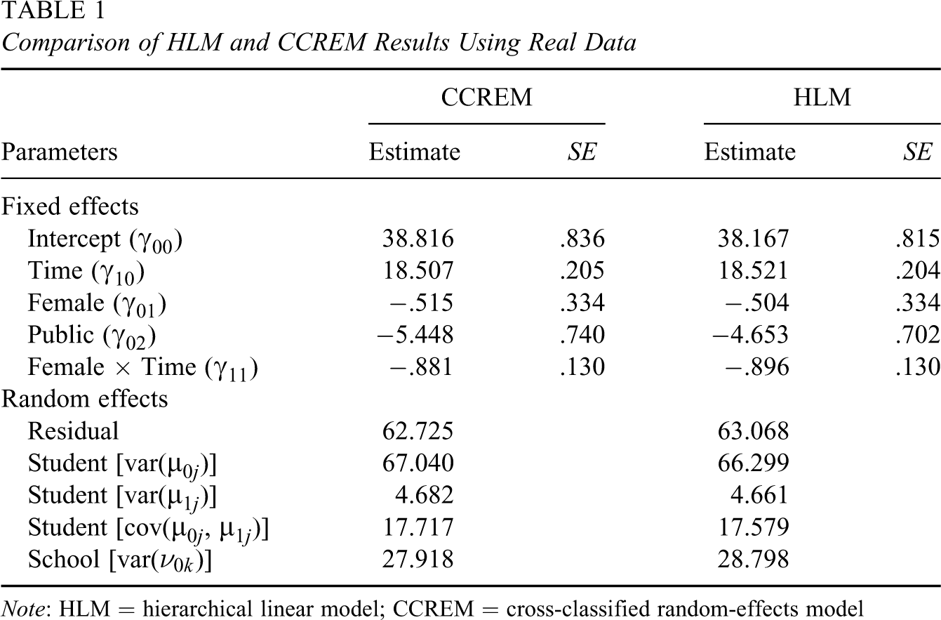
Note: HLM = hierarchical linear model; CCREM = cross-classified random-effects model

With real data analysis, we do not know the true population parameters. Therefore, it is unknown whether the differences we observed between the results from the CCREM and the HLM analyses were simply due to sampling error. In addition, because we cannot manipulate the mobility rate in real data analysis, it is unknown how different the results would be if the mobility rate is higher. Therefore, we conducted the following simulation studies to further investigate the impacts of ignoring students' mobility, considering a number of design factors such as the number of schools and students per school, mobility rate, and the magnitude of the variances of different random effects.

Simulation I

There are many factors affecting students’ school switching. Students may move due to completion of an academic program, such as graduating from middle schools and entering high schools. In this case, it is likely that a subsample of students switches schools simultaneously at a certain time point. In the first simulation study, we examined the mobility pattern in which students only switch schools once between the first and the second assessment occasions. We presented the procedures for data generation and analyses, followed by results.

Method

Data generation

The data were generated using SAS 9.1 (SAS Institute Inc., 2004). The model used for data generation was a two-level cross-classified growth model:

Level 1 : y_{t (j k)} = π_{0 (j k)} + π_{1 (j k)} x_{t (j k)} + ϵ_{t (j k)},

\begin{aligned} Level 2 : π_{0 (j k)} & = γ_{00} + γ_{01} w_{j} + γ_{02} z_{k} + μ_{0 j} + ν_{0 k} \\ - 1.7 p c π_{1 (j k)} = γ_{10} + γ_{11} w_{j} + μ_{1 j}, \end{aligned}

where t indexed the occasions (t = 1, 2, 3, 4), j indexed students (j = 1, …, J), and k indexed schools (k = 1, …, K). The time variable

x_{t (j k)}

in the Level 1 model took on values of 0, 1, 2, and 3 corresponding to Occasions 1, 2, 3, and 4, respectively. The Level 1 residual

ϵ_{t (j k)}

was generated to be normally distributed with mean of 0 and variance of .40 (σ² = .40). The Level 2 model included a student-specific time-invariant predictor w_j (e.g., IQ) and a school-specific time-invariant predictor z_k (e.g., teacher–student ratio¹). Both w_j and z_k were generated using the standard normal distribution. The student random effects

μ_{0 j}

and

μ_{1 j}

were generated using a bivariate normal distribution with mean of 0 and variances and covariance of

ψ = [\begin{matrix} ψ_{00} & ψ_{01} \\ ψ_{10} & ψ_{11} \end{matrix}]

. The school random effect

ν_{0 k}

was generated to be normally distributed with mean of 0 and variance of τ. The magnitude of

ψ

and τ was manipulated to vary under different conditions. The overall intercept

γ_{00}

was generated with the value of .10. The regression coefficients

γ_{01}

γ_{02}

, and

γ_{10}

, which represented the effects of student-specific predictor w_j , school-specific predictor z_k , and the time variable

x_{t (j k)}

, respectively, were generated with the value of .50. The regression coefficient

γ_{11}

, which represented the cross-level interaction effect between the time variable and the student-specific predictor (i.e.,

w_{j} x_{t (j k)}

) was also generated with value of .50.

Design Factors

Five design factors were considered in the study, including (a) the number of schools, (b) the number of students per school at Occasion 1, (c) mobility rate, (d) variances and covariance of the student random effects ( $ψ$ ), and (e) variance of the school random effects (τ).

The number of schools

A recent systematic review of 27 studies using multilevel models conducted by Graves and Frohwerk (2009) in School Psychology Quarterly showed that the average number of schools used in those studies was 28 with the 25th and 75th percentiles of 3 and 36, respectively. Thus, we used 25 and 50 schools as the two levels in this design factor.

The number of students per school at occasion 1

Based on Graves and Frohwerk’s review, the average number of students per school was 44 with a standard deviation of 43. Hence we selected 50 versus 100 students per school as the two levels in this design factor. The overall number of students, based on these simulation conditions, ranged from 1,250 (50 × 25) to 5,000 (100 × 50), which covered a reasonable range of sample sizes for multilevel growth models in educational studies.

Mobility rate

Despite the requirement of the No Child Left Behind Act (NCLB) that mandates student mobility be taken into account when rating schools, there is surprisingly little standardization in the definition and computation of mobility rate (Demie, 2002). In this study, the term student mobility was defined as a student switching school between two assessment occasions. The mobility rate of a school was calculated as the ratio between the number of students leaving the school and the total number of students in the school. According to the 1998 National Assessment of Educational Progress (NEAP), one third of 4th graders, 19% of 8th graders, and 10% of 12th graders changed schools at least once in the previous 2 years. Hence, we selected three levels of mobility rate, 5%, 20%, and 35%, to represent low, medium, and high mobility rate, respectively.

Variance and covariance of student random effects ()

Based on the criteria provided by Raudenbush and Liu (2001), we used $ψ = [\begin{matrix} .20 & .05 \\ .05 & .10 \end{matrix}]$ as the medium size of the variance–covariance matrix of the student-level random effects, and $ψ = [\begin{matrix} .10 & .025 \\ .025 & .05 \end{matrix}]$ as the small size.

Variance of school random effects (τ)

Following previous simulation studies (Meyers & Beretvas, 2006; Moerbeek, 2004), two levels were chosen for this factor: (a) a small size with τ = .1 and (b) a medium size with τ = .2. The intraclass correlation (ICC) for schools, computed by $ICC = τ / (σ^{2} + ψ_{00} + τ)$ , was .14 for medium $ψ$ and small τ, .28 for medium $ψ$ and medium τ, .17 for small $ψ$ and small τ, and .34 for small $ψ$ and medium τ. These ICCs represented a range of clustering effects that are commonly seen in multilevel data (Hedges & Hedberg, 2007; Hox, 2002).

Combining these five factors, this study involved 48 conditions. For each condition, 200 data sets were generated. A total of 9,600 data sets were generated for the analyses. Using the lmer function in the R package lme4 (Bates & Sarkar, 2007), each data set was analyzed with two models: (a) the correct model, that is, the cross-classified model used to generate the data; and (b) the misspecified model, in which students' mobility was ignored. More specifically, the misspecified model was a three-level strictly HLM assuming that repeated measures were nested within students and students were nested within their Time 1 schools, as follows:

Level 1 : y_{t (j k)} = π_{0 (j k)} + π_{1 (j k)} x_{t (j k)} + ϵ_{t (j k)},

\begin{aligned} Level 2 : π_{0 (j k)} & = θ_{0 (j k)} + γ_{01} w_{j k} + μ_{0 j} \\ π_{1 (j k)} & = θ_{1 (j k)} + γ_{11} w_{j k} + μ_{1 j}, \end{aligned}

\begin{array}{l} Level 3: θ_{0 k} = γ_{00} + γ_{02} z_{k} + ν_{00 k} \\ θ_{1 k} = γ_{10} . \end{array}

Analysis

Following the recommendations by Burton, Altman, Royston, and Holder (2006) on designing simulation studies, we examined the relative bias, accuracy, and coverage of the parameter estimates.

Relative bias

For both the fixed effects and the variance components, we computed the relative bias of the estimates by

B (\hat{θ}) = \frac{\hat{θ} - θ}{θ},

where

\hat{θ}

is the parameter estimate and θ is the true parameter value. A negative relative bias indicates an underestimation of the parameter (i.e., the estimated value is smaller than the true parameter value), whereas a positive relative bias indicates an overestimation of the parameter (i.e., the estimated value is larger than the true parameter value). For fixed effects, we also computed the relative bias of standard error estimates by

B ({\hat{S}}_{\hat{θ}}) = \frac{{\hat{S}}_{\hat{θ}} - {\hat{S}}_{\hat{θ}_EMP_TRUE}}{{\hat{S}}_{\hat{θ}_EMP_TRUE}},

where

{\hat{S}}_{\hat{θ}}

is the estimated standard error and

{\hat{S}}_{\hat{θ}_EMP_TRUE}

is the true model empirical standard error, calculated as the standard deviation of the 200 estimates in the true model. Using the cutoff value recommended by Hoogland and Boomsma (1998), relative bias that has an absolute value of .05 or less was considered acceptable. We did not examine the relative bias of the standard error estimates of the variance components because it is not advised to use the Wald test for variance components (e.g., Fears, Benichou, & Gail, 1996).

Analysis of variance (ANOVA) was used to partition the total variation of the observed relative biases to determine the effects of the five design factors. Given that the purpose of using ANOVA in the present study was descriptive rather than inferential, the p value of the F test was not reported. Instead, the eta-squared (η²) effect size² was computed and reported as a measure of practical significance. Only effects with η² greater than .01 were reported.

Accuracy

The square root of mean square error (SRMSE) was used as a measure of the overall accuracy of a parameter estimate. It was computed by

SRMSE = \sqrt{{(\bar{\hat{θ}} - θ)}^{2} + {\hat{S}}_{\hat{θ}_EMP}^{2}},

where

\bar{\hat{θ}}

was the mean of a parameter estimate over the 200 replications and

{\hat{S}}_{\hat{θ}_EMP}

was the empirical standard error. The SRMSE of a parameter estimate in the misspecified model was compared with that in the true model. A larger SRMSE indicates less accuracy in the estimate.

Coverage

The coverage of a confidence interval is the proportion of obtained confidence intervals that include the specified true parameter value. The 95% confidence interval for a fixed effect was computed as $\hat{θ} \pm Z_{1 - 0.5 / 2} {\hat{S}}_{\hat{θ}}$ ( $z_{1 - 0.5 / 2}$ = 1.96).The coverage rate of a 95% confidence interval should be approximately equal to .95, with a margin of error of .03.³ In other words, between 92% and 98% of the obtained confidence intervals should contain the true parameter value. A coverage rate that is higher than 98% indicates decreased power or inflated Type II error rate as more replications will fail to find significant results. A coverage rate that is lower than 92% indicates inflated Type I error rate as more replications will incorrectly find significant results. The confidence interval was only computed for fixed effects.

Results

Variance Components

In both the correct and the misspecified model, there were five variance components, including variance of the school random effects (τ), variance of the student random effects associated with the intercept ( $ψ_{00}$ ), variance of the student random effects associated with the growth rate ( $ψ_{11}$ ), covariance of the two student random effects ( $ψ_{01}$ ), and the within-student residual variance (σ²). In the correct model, the relative biases of the parameter estimates were all smaller than the recommended cutoff values, which indicated that all the generated data were close to the intended data-generating model. In the misspecified model, the variance of school random effects (τ) was generally underestimated, whereas $ψ_{11}$ and $ψ_{01}$ were overestimated. In addition, the accuracy of the estimates of τ, $ψ_{11}$ , and $ψ_{01}$ decreased in the misspecified model. Interestingly, estimates of $ψ_{00}$ and σ² were generally unbiased.

Estimated variance of the school random effects (τˆ)

In general, the variance of school random effects was underestimated. When the mobility rate was 5%, the relative bias was small and acceptable. As the mobility rate increased to 20% and 35%, the relative bias became larger, ranging from −.149 to −345.⁴ The accuracy of the estimate also decreased in the misspecified model compared to that in the true model when mobility rate was high. The average SRMSE at the high mobility rate (35%) was .037 in the true model and .054 in the misspecified model. ANOVA results showed that mobility rate accounted for about 20% of the total variation in the observed relative bias (η² = .19).

Estimated variance of the student random effects associated with the growth rate (ψˆ11)

When the mobility rate was 5%, the relative bias in ${\hat{ψ}}_{11}$ was acceptable. When the mobility rate increased to 20%, small positive relative bias emerged [B( ${\hat{ψ}}_{11}$ ) = .08] under conditions of medium variance of school random effects (τ = .2) and small $ψ$ matrix (i.e., variance and covariance of student random effects). When the mobility rate increased to 35%, the positive relative bias became apparent under almost all conditions, ranging from .037 to .165. The accuracy of the estimate also slightly decreased at the high mobility rate (mean SRMSE = .005 in the true model and mean SRMSE = .008 in the misspecified model).

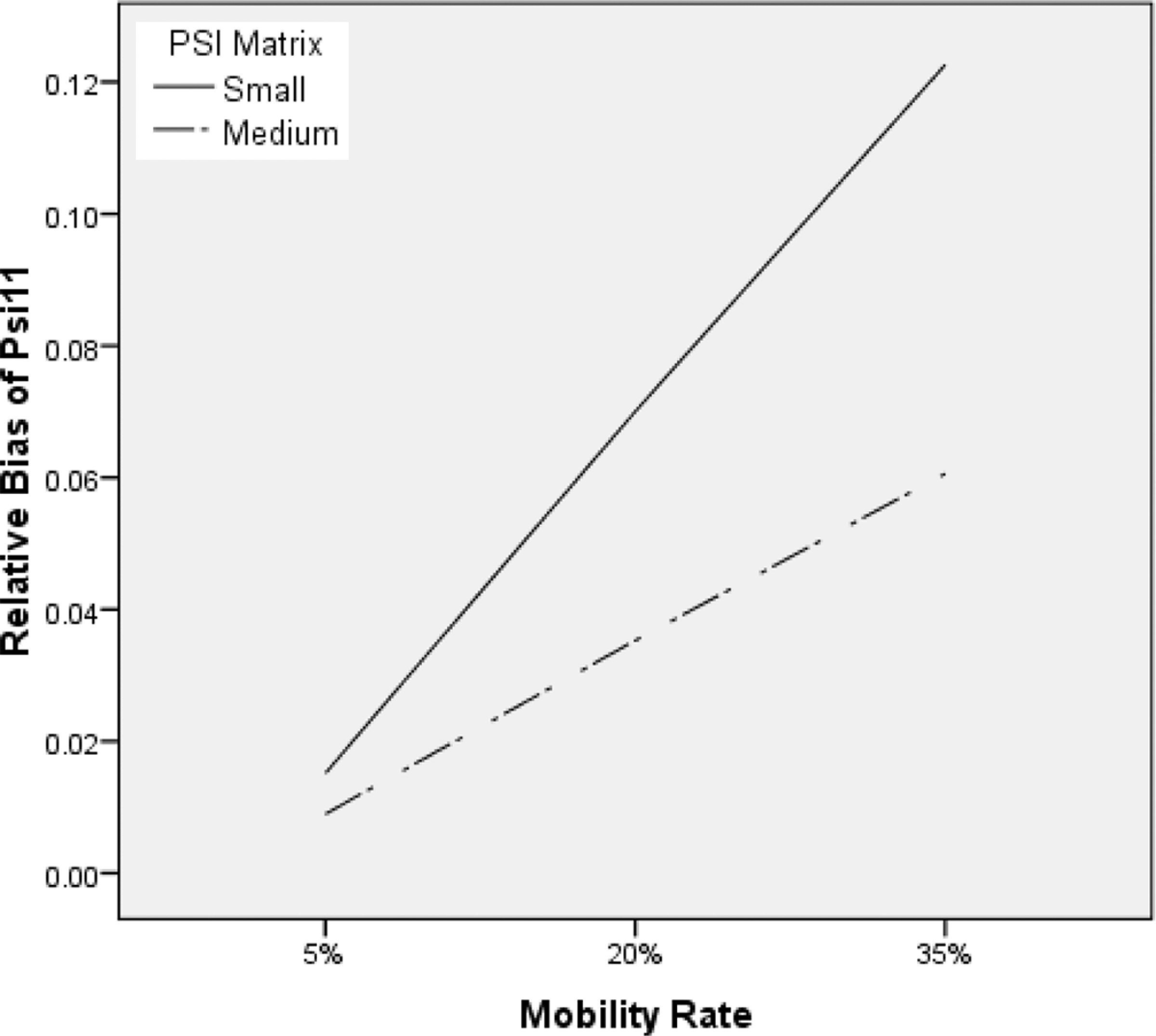
The ANOVA results indicated that mobility rate was the most important factor influencing the observed relative bias (η² = .14). The increase in the mobility rate caused larger relative bias in ${\hat{ψ}}_{11}$ . The magnitude of the $ψ$ matrix and τ had small effects on the relative bias (η² = .04 and .03, respectively). The smaller the $ψ$ matrix, the greater the relative bias was. On the other hand, as τ increased the relative bias became larger. There was a noteworthy interaction effect between mobility rate and the magnitude of $ψ$ (η² = .02). The effect of the $ψ$ matrix became larger when mobility rate increased (see Figure 3 ).

Figure 3.

Effects of the mobility rate and ψ on the relative bias of ${\hat{ψ}}_{11}$ . Note: ψ is the covariance matrix of student random effects; ${\hat{ψ}}_{11}$ is the estimated variance of student random effects associated with the growth rate.

Estimated covariance of the student random effects (ψˆ01)

In general, there was a positive relative bias in ${\hat{ψ}}_{01}$ , ranging from .006 to .591. The accuracy of the estimate decreased in the misspecified model when the mobility rate was high. The average SRMSE of ${\hat{ψ}}_{01}$ when mobility rate equal to 35% was .006 in the true model and .013 in the misspecified model. The ANOVA results indicated that mobility rate explained about 18% of the variation of the relative bias in ${\hat{ψ}}_{01}$ . The magnitude of τ and the $ψ$ matrix had small effects (η² = .07 and .06, respectively). Larger τ and smaller $ψ$ were related to larger relative biases. There was an interaction effect between the mobility rate and the magnitude of $ψ$ (η² = .02). As the mobility rate increased, the increase of the relative bias was greater with smaller $ψ$ (see Figure 4 ). Another noteworthy interaction effect between mobility rate and the magnitude of τ (η² = .02) indicated that as the mobility rate increased, the increase of the relative bias was greater with larger τ (see Figure 5 ).

Figure 4.

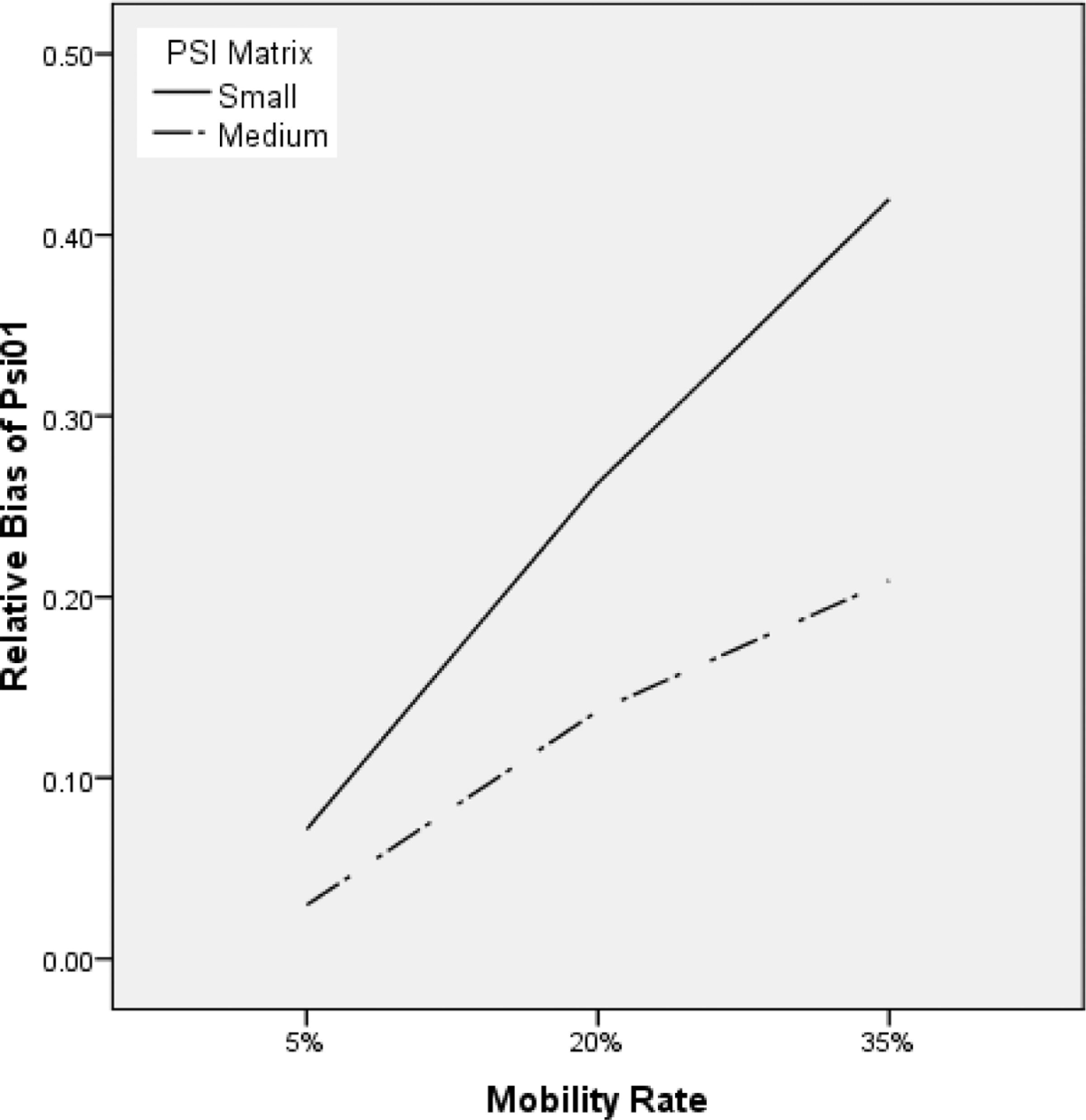
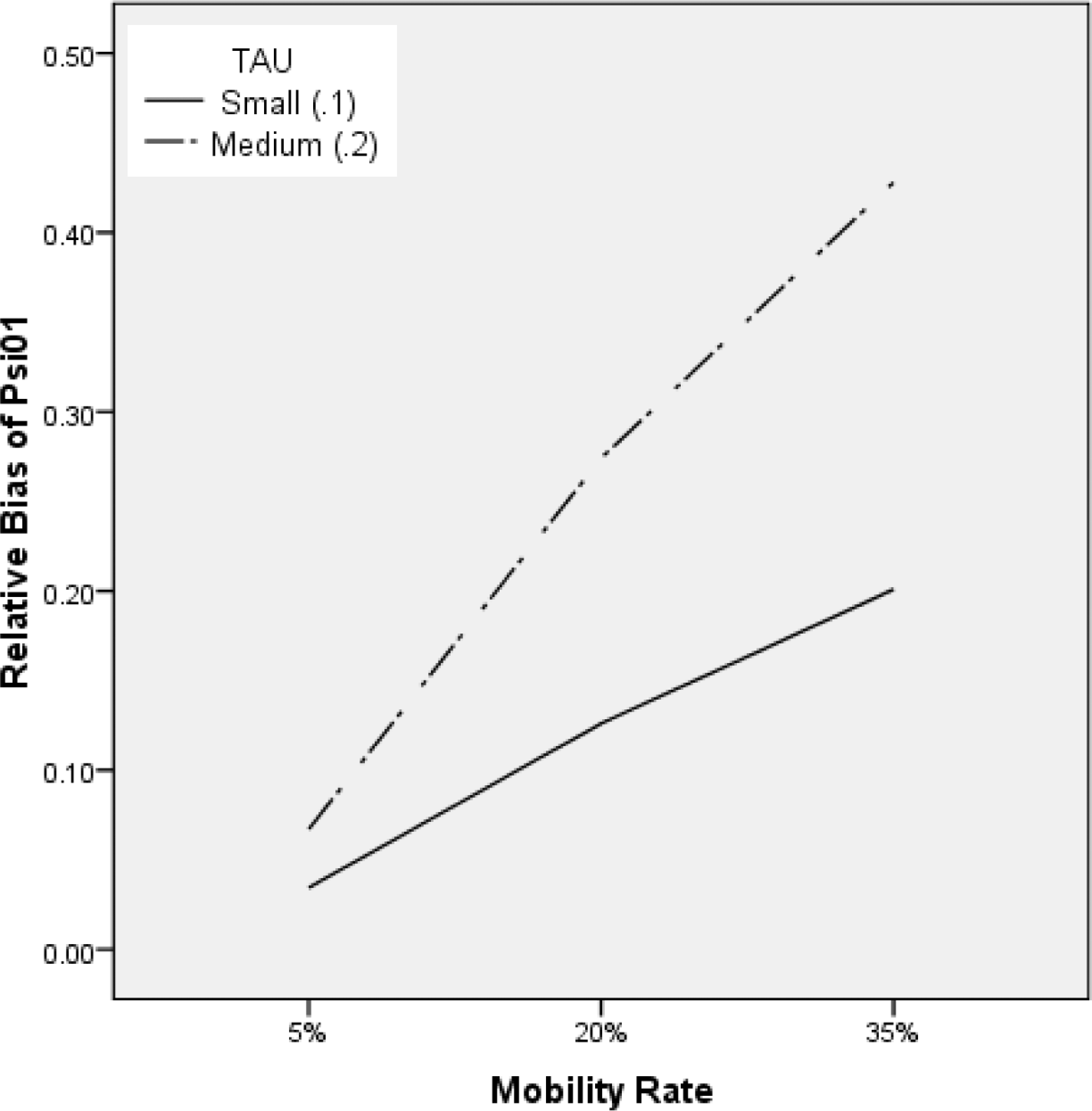
Effects of the mobility rate and ψ on the relative bias of ${\hat{ψ}}_{01}$ . Note: ψ is the covariance matrix of student random effects; ${\hat{ψ}}_{01}$ is the estimated covariance of student random effects.

Figure 5.

Effects of the mobility rate and τ on the relative bias of $ψ_{01}$ . Note: τ is the variance of school random effects; ${\hat{ψ}}_{01}$ is the estimated covariance of student random effects.

Fixed Effects

The estimates of the fixed effects themselves remained consistent under the misspecified model because the consistency of generalized least squares (GLS) estimator does not depend on the specification of the random effects of the model (Kreft & de Leeuw, 1998). However, the standard error of the intercept ( ${\hat{S}}_{{\hat{γ}}_{00}}$ ) and the standard error of the regression coefficient associated with the school-specific predictor z ( ${\hat{S}}_{{\hat{γ}}_{02}}$ ) were biased, which in turn affected the coverage rate the 95% confidence interval on the two fixed effects.

Estimated intercept (γˆ00) and the corresponding standard error

In general, the standard error of the intercept ( ${\hat{S}}_{{\hat{γ}}_{00}}$ ) was underestimated, with the negative relative bias up to −.288. The ANOVA results showed that the mobility rate had the largest effect on the relative bias (η² = .21). As expected, the larger the mobility rate, the greater the relative bias in the estimated standard error of the intercept was. The number of schools also had a small effect (η² = .04) on the observed relative bias. As the number of schools increased, the relative bias became smaller. In addition, in the misspecified model, the coverage rate of the 95% confidence interval reduced to 91% when mobility rate was 20% and further decreased to 88% as mobility rate increased to 35%.

Estimated regression coefficient of the school-specific predictor (γˆ02) and the corresponding standard error

The standard error associated with the school-specific covariate had a moderate to large negative relative bias (or underestimation) under all conditions, ranging from −.197 to −.813. The mobility rate had the largest effect (η² = .61). As expected, the larger the mobility rate, the greater the relative bias in ${\hat{S}}_{{\hat{γ}}_{02}}$ was. The number of student per school had the second largest effect (η² = .13). As the number of students per school increased, the relative bias became larger. The magnitude of the variance of school random effects (τ) had a small effect (η² = .09). Larger variance of school random effects was associated with greater relative bias. The magnitude of the $ψ$ matrix (i.e., variances and covariance of student random effects) also had a small effect on the relative bias (η² = .01). The relative bias in ${\hat{S}}_{{\hat{γ}}_{02}}$ was greater when $ψ$ was small. Similarly, the 95% confidence interval had substantial undercoverage in the misspecified model. The observed coverage rate was only 70% when the mobility rate was 5%. The coverage rate reduced to 49% when the mobility rate was 20%, and further reduced to 41% when the mobility rate was 35%.

Simulation II

Method

The first simulation study mimicked the type of students' mobility that was prompted by program design. Students also move for all kinds of other reasons, such as temporary housing, change of parents' occupation, family breakdown, and poverty. In those cases, students may switch schools at any time point, and a student can switch schools for multiple times. In the second simulation study, we generated data to mimic the more complicated situation. At each assessment occasion, a group of students was randomly selected to switch schools. In the generated data, some students move only once and some move more than once. Based on the findings from the first simulation study, the high mobility rate and the magnitude of τ and the $ψ$ matrix had substantial impact on the estimation of the model parameters and the corresponding standard errors. Thus, we selected the specific condition with high mobility rate (35%), 50 schools, 100 students per school, medium τ (τ = .2), and small $ψ$ matrix $(ψ = [\begin{matrix} .10 & .025 \\ .025 & .05 \end{matrix}])$ to further examine the impact of a different mobility pattern (i.e., students changed schools at any time and for multiple times).

Results

The results had some similarities with those in the first simulation study. More specifically, τ was underestimated [B( $\hat{τ}$ ) = −.400], whereas $ψ_{11}$ and $ψ_{01}$ were overestimated [ $B ({\hat{ψ}}_{11})$ = .390, $B ({\hat{ψ}}_{01})$ = .280]. The standard errors of the intercept and the regression coefficient of the school-level predictor were underestimated [B( ${\hat{S}}_{{\hat{γ}}_{00}}$ ) = −.210, B( ${\hat{S}}_{{\hat{γ}}_{02}}$ ) = −.910], resulting in an undercoverage of the 95% confidence interval for the two parameters.

There were also important differences in the results. First, the variance of the student random effects associated with the intercept was underestimated [ $B ({\hat{ψ}}_{00})$ = −.170] and the residual variance was overestimated [B( ${\hat{σ}}^{2}$ ) = .150], whereas in the first simulation study the estimates of both parameters were unbiased. Second, positive relative biases were found in the estimated standard errors of the regression coefficients of the time variable x [B( ${\hat{S}}_{{\hat{γ}}_{10}}$ ) = .091], the student-level predictor w [B( ${\hat{S}}_{{\hat{γ}}_{01}}$ ) = .072], and the cross-level interaction xw [B( ${\hat{S}}_{{\hat{γ}}_{11}}$ ) = .210]. These positive relative biases led to overcoverage of the 95% confidence interval for the parameters. In other words, the positive relative biases (or overestimations) in the standard errors resulted in the reduction of the statistical power for testing the corresponding fixed effects.

Discussion and Conclusions

Multilevel models are widely used in educational research to model growth. If students stay in the same school overtime, the data structure is strictly hierarchical with repeated measures nested within students and students nested within schools. On the other hand, if students switch schools, the structure of the data becomes cross-classified with repeated measures cross-classified by students and schools. This study showed that treating the multilevel cross-classified data structure as strictly hierarchical led to the misspecification in the design matrix of the school random effects, and such misspecification could cause biases in the variance components estimates and the standard error estimates of the fixed effects. It was found that depending on the pattern of student mobility, the direction and magnitude of observed relative biases changed dramatically.

Pattern of Student Mobility

Students move in different patterns. In the first simulation, students switch schools altogether at a particular time point simultaneously (pattern I), whereas in the second simulation, students switch schools at any time point, and some students switch schools more than once (pattern II).

The pattern of student mobility is related to the degree of cross-classification. According to Luo and Kwok (2009), there were complete versus partial cross-classification. In completely cross-classified data, units in a cluster of one crossed factor could affiliate with any clusters of the other crossed factor and vice versa. On the other hand, in partial cross-classified data, units in a cluster of one crossed factor can only affiliate with part of the clusters of the other crossed factor. Most cross-classified longitudinal data are partially cross-classified because (a) only some of the students change schools and (b) students do not switch schools at every time point. Only in a very rare scenario in which all students are shuffled to different schools at all time points can the data be deemed as completely cross-classified.

Both patterns of mobility (I and II) investigated in this study produced partially cross-classified data. Pattern I produced a partially cross-classified data structure that was closer to the hierarchical structure, whereas pattern II produced structure that was closer to the completely cross-classified structure. The difference can be seen from the design matrix for school random effects. In pattern I, the correct design matrix takes such form as⁵

$[\begin{matrix} 1 & 0 & 0 & \dots & 0 \\ 0 & 1 & 0 & \dots & 0 \\ 0 & 1 & 0 & \dots & 0 \\ 0 & 1 & 0 & \dots & 0 \end{matrix}]$ for a student who only switches school once. In pattern II, the correct design matrix takes such form as $[\begin{matrix} 1 & 0 & 0 & 0 & 0 & \dots & 0 \\ 0 & 1 & 0 & 0 & 0 & \dots & 0 \\ 0 & 0 & 1 & 0 & 0 & \dots & 0 \\ 0 & 0 & 0 & 1 & 0 & \dots & 0 \end{matrix}]$ for a student who switches schools at all four time points. Apparently, the former design matrix is closer to the design matrix used in the misspecified HLM model (i.e., $[\begin{matrix} 1 & 0 & 0 & \dots & 0 \\ 1 & 0 & 0 & \dots & 0 \\ 1 & 0 & 0 & \dots & 0 \\ 1 & 0 & 0 & \dots & 0 \end{matrix}]$ ) than the latter one.

Redistribution of Variance Components

Knowing the relationship between mobility pattern and degree of cross-classification helps us to understand the mechanism of the redistribution of the variance components and to link the findings of this study to previous research findings. In both patterns I and II, model misspecification causes part of the school variance to redistribute to the other levels, leading to underestimation of the school-level variance component. In pattern I, the redistributed school variance is added to the student level, causing overestimation of the variance of students random effects associated with the growth rate ( $ψ_{11}$ ) and the covariance of students random effects associated with the initial status and the growth rate ( $ψ_{01}$ ). However, the residual variance at the repeated-measure level is unaffected. In pattern II, the redistributed school variance is not only added to the student level causing the overestimated $ψ_{11}$ and $ψ_{01}$ but also added to the repeated measure level causing the overestimated residual variance. In addition, the variance of students random effects associated with the intercept ( $ψ_{00}$ ) is underestimated.

These findings have some similarities with those of previous studies in which a crossed factor was completely omitted in the misspecified model (i.e., the design matrix for school random effects was misspecified as a zero matrix). It has been shown that when the remaining crossed factor is almost nested within the omitted crossed factor, a situation similar to pattern I, almost all of the variance component of the omitted factor is added to the variance component of the remaining crossed factor, and little is added to the level below (Luo & Kwok, 2009). On the other hand, when the remaining crossed factor is more cross-classified with the omitted crossed factor, a situation similar to pattern II, all the variance component of the omitted factor is added to the level below, and some variance of the remaining crossed factor is also redistributed to the level below.

Standard Error Estimates of the Fixed Effects

The covariance matrix of the maximum likelihood estimator of the fixed effects γ as in Equation 1 is given by cov( $\hat{γ}$ ) = (Z′V ⁻¹ Z)⁻¹ (Longford, 1993), where V is the covariance matrix of y and is given by V = XGX′ + R, where $X = [\begin{matrix} X_{a} & 0 \\ 0 & X_{b} \end{matrix}]$ ⁶ R = σ² I, and $G = [\begin{matrix} ψ_{00} & ψ_{10} \\ ψ_{01} & ψ_{11} & 0 \\ ⋱ \\ ψ_{00} & ψ_{10} \\ ψ_{01} & ψ_{01} \\ τ \\ 0 & ⋱ \\ τ \end{matrix}]$ . We can see that the variances of the estimated fixed effects depend not only on the variance components, but also on the design matrix X. Because the design matrix X can have an infinite number of forms when the numbers of schools, students, and repeated measures are large without any restriction on the switching activity (i.e., students are allowed to move at any time point to any school), we only examined the design matrices corresponding to the two representative mobility patterns (i.e., pattern I and pattern II). Under both mobility patterns, the standard errors of the intercept and the regression coefficient of the predictor at the school level were underestimated. This is similar to previous findings that the standard errors of the intercept and the regression coefficients of the predictor variables associated with the ignored crossed factor are generally underestimated when a crossed factor is completely omitted (Luo & Kwok, 2009).

Under pattern I (i.e., students move once simultaneously), no substantial relative biases have been found in the standard error estimates of the regression coefficients of the time variable x, the student-level predictor w, and the cross-level interaction xw. However, under pattern II (i.e., students move multiple times), positive relative biases have been found in those standard error estimates. We drew upon mixed model theories to explain these differences. According to Berkhof and Kampen (2004), the standard error of the regression coefficient of the student-level predictor is a weighted sum of the Level 1 residual variance (σ²) and the variance of the student random effects associated with the intercept ( $ψ_{00}$ ). Under pattern I, the estimated standard error of the regression coefficient of the student-level predictor is unbiased because both σ² and $ψ_{00}$ are unbiased. Under pattern II, σ² is overestimated and $ψ_{00}$ is underestimated; however, the weighted sum of the two still increases, causing the positively biased standard error estimate of the regression coefficient of the student-level predictor.

For the regression coefficients of the time variable x and the cross-level interaction xw, their standard errors are the weighted sums of the Level-1 residual variance (σ²) and the variance of the student random effects associated with the slope ( $ψ_{11}$ ; Berkhof, 2000; Berkhof & Kampen, 2004). Under pattern I, we did not find substantial relative biases in the estimated standard errors in the simulation study because only $ψ_{11}$ was slightly overestimated [B( ${\hat{ψ}}_{11}$ ) ≤ .16], which did not have a substantial impact on the standard error estimates. However, under pattern II, both σ² and $ψ_{11}$ were overestimated, leading to a substantial positive relative bias in the standard error estimates.

The Use of School Switching as a Student-Level Predictor

Previous research has demonstrated that children whose families live in poverty are more likely to move and that student mobility has a negative impact on academic achievement at all levels (e.g., Demie, 2002; Kerbow, 1996). Given that switchers and non-switchers may not come from the same population, it is important to take the school-switching status (i.e., “having switched schools or not”) into consideration. However, some researchers have the misconception that including a covariate of school-switching status would be a remedy for not considering the cross-classified structure of the data. In a supplementary simulation,⁷ we examined the effect of ignoring cross-classification but including the school-switching status covariate. Similar biases were found in parameter estimates. In addition, because school-switching status is a student-level predictor, its standard error is overestimated in the misspecified model, causing a reduced statistical power in detecting the effect of the variable. Therefore, simply including the covariate of school-switching status does not help to reduce biases.

Implications

In longitudinal multilevel studies, it is common that participants change group membership or move to different clusters over time. In some circumstances, researchers may not have participants' cluster identifications at every time point; therefore, they may not be able to adequately analyze their data with CCREMs. To assess the potential impact of ignoring student mobility, researchers should consider three factors: the target of the analysis, the rate of mobility, and the pattern of mobility. If the target of the analysis is on testing the overall intercept and the effect of a school-level predictor, it is likely to have spurious significant results (i.e., inflated Type I error rates) under the misspecified model even when the mobility rate is relatively low. If the target of the analysis is on testing the overall growth rate and the effect of a student-level predictor on the intercept and growth rate, it is likely to have reduced power (i.e., inflated Type II error rates) when the mobility pattern is more spread out (i.e., students switch schools at any time and multiple times) and the mobility rate is relatively high. In addition, model misspecification will have a larger impact when there is a large variance at the school level and a relatively small variance at the student level.

Limitations

The present study only provided a preliminary investigation of the impact of misspecifying CCREMs in cross-classified longitudinal data. A major limitation is that the CCREM used in the study assumed that the effect of a particular school disappears when students move out of the school. In other words, it was assumed that there was no cumulative school effect. It should be noted that there are less restrictive CCREMs that allow for cumulative school effects (Grady & Beretvas, 2010; McCaffrey, Lockwood, Koretz, & Hamilton, 2004; Raudenbush & Bryk, 2002). Additionally, we only considered a simple linear growth model for the repeated measures that may not be applicable especially for multiwave longitudinal studies (Kwok, Luo, & West, 2010). Similarly, in the simulation studies, we assumed a very simple error structure (i.e., identity structure: V(ϵ_t(jk)) = σ²I) for the within-subject repeated measures, which may not be always suitable for longitudinal data (Kwok et al., 2008; Kwok, West, & Green, 2007). Future research could investigate the impacts of ignoring the cross-classified structure in longitudinal multilevel data with less restrictive assumptions.

Footnotes

Notes

References

Bates

(2004). Sparse matrix representations of linear mixed models. Retrieved May 1, 2007, from http://www.stat.wisc.edu/%7Ebates/reports/MixedEffects.pdf

Bates

(2005). Fitting linear mixed models in R using the lme4 package. R Newsletter, 5, 27–30.

Bates

Sarkar

(2007). The lme4 package. Retrieved May 14, 2007, from http://cran.r-project.org/doc/packages/lme4.pdf

Berkhof

(2000). Specification methods for the multilevel model Leiden, Netherlands: DSWO Press.

Berkhof

Kampen

J. K.

(2004). Asymptotic effect of misspecification in the random part of the multilevel model. Journal of Educational and Behavioral Statistics, 29, 201–218.

Burton

Altman

D.G.

Royston

Holder

R. L.

(2006). The design of simualtion studies in medical statistics. Statistics in Medicine, 25, 4279–4292.

De Fraine

Van Landeghem

Van Damme

Onghena

(2005). An analysis of well-being in secondary school with multilevel growth curve models and multilevel multivariate models. Quality and Quantity, 39, 297–316.

Demie

(2002). Pupil mobility and educational achievement in schools: An empirical analysis. Educational Research, 44, 197–215.

Fears

T. R.

Benichou

Gail

M. H.

(1996). A reminder of the fallibility of the Wald statistic. The American Statistician, 50, 226–227.

10.

Fielding

(2002). Teaching groups as foci for evaluating performance in cost-effectiveness of GCE Advanced Level provision: Some practical methodological innovations. School Effectiveness and School Improvement, 13, 225–246.

11.

George

Thomas

(2000). Victimization among middle and high school students: A multilevel analysis. The High School Journal, 84, 48–57.

12.

Goldstein

(1986). Multilevel mixed linear model analysis using iterative generalized least squares. Biometrika, 73, 43–56.

13.

Goldstein

(1995). Multilevel statistical models London, UK: Edward Arnold.

14.

Grady

M. W.

Beretvas

S. N.

(2010). Incorporating student mobility in achievement growth modeling: A cross-classified multiple membership growth curve model. Multivariate Behavioral Research, 45, 393–419.

15.

Graves

Frohwerk

(2009). Multilevel modeling and school psychology: A review and practical example. School Psychology Quarterly, 24, 84–94.

16.

Hedges

Hedberg

E. C.

(2007). Intraclass correlation values for planning group-randomized trials in education. Educational Evaluation and Policy Analysis, 29, 60–87.

17.

Hill

P. W.

Goldstein

(1998). Multilevel modeling of educational data with cross-classification and missing identification for units. Journal of Educational and Behavioral Statistics, 23, 117–128.

18.

Hoogland

J. J.

Boomsma

(1998). Robustness studies in covariance structure modeling. Sociological Methods and Research, 26, 329–367.

19.

Hox

(2002). Multilevel analysis: Techniques and applications Mahwah, NJ: Lawrence Erlbaum.

20.

Jayasinghe

U. W.

Marsh

H. W.

Bond

(2003). A multilevel cross-classified modeling approach to peer review of grant proposals: The effects of assessor and researcher attributes on assessor ratings. Journal of the Royal Statistical Society: Series A, 166, 279–300.

21.

Kerbow

(1996). Patterns of urban student mobility and local school reform. Journal of Education for Students Placed at Risk, 1, 147–169.

22.

Kreft

de Leeuw

(1998). Introducing multilevel modeling Thousand Oaks, CA: Sage.

23.

Kwok

Luo

West

S. G.

(2010). Using modification indices to detect turning points in longitudinal data: A Monte Carlo study. Structural Equation Modeling, 17, 216–240.

24.

Kwok

Underhill

A. T.

Berry

J. W.

Luo

Elliott

T. R.

Yoon

(2008). Analyzing longitudinal data with multilevel models: An example with individuals living with lower extremity intra-articular fractures. Rehabilitation Psychology, 53, 370–386.

25.

Kwok

West

S. G.

Green

S. B.

(2007). The impact of misspecifying the within-subject covariance structure in multiwave longitudinal multilevel models: A Monte Carlo study. Multivariate Behavioral Research, 42, 557–592.

26.

Longford

N. T.

(1993). Random coefficient models. Oxford: Clarendon Press.

27.

Luo

Kwok

(2009). The impacts of misspecifying cross-classified random effects models. Multivariate Behavioral Research, 44, 182–212.

28.

(2004). Modeling stability of growth between mathematics and science achievement during middle and high school. Evaluation Review, 38, 104–122.

29.

McCaffrey

D. F.

Lockwood

J. R.

Koretz

Hamilton

(2004). Models for value-added modeling of teacher effects. Journal of Educational and Behavioral Statistics, 29, 67–101.

30.

McCoach

D. B.

O’Connel

A. A.

Reis

S. M.

Levitt

H. A.

(2006). Growing readers: A hierarchical linear model of children’s reading growth during the first 2 years of school. Journal of Educational Psychology, 98, 14–28.

31.

Meyers

Beretvas

S. N.

(2006). The impact of inappropriate modeling of cross-classified data structures. Multivariate Behavioral Research, 41, 473–497.

32.

Moerbeek

(2004). The consequence of ignoring a level of nesting in multilevel analysis. Multivariate Behavioral Research, 39, 129–149.

33.

Rasbash

Goldstein

(1994). Efficient analysis of mixed hierarchical and cross-classified random structures using a multilevel model. Journal of Educational and Behavioral Statistics, 19, 337–350.

34.

Rasbash

Steele

Browne

Goldstein

(2009). A user’s guide to MLwiN 2.10 Bristol, UK: Center for Multilevel Modeling.

35.

Raudenbush

S. W.

(1993). A crossed random effects model for unbalanced data with applications in cross-sectional and longitudinal research. Journal of Educational Statistics, 18, 321–349.

36.

Raudenbush

S. W.

Bryk

A. S.

(2002). Hierarchical linear models: Applications and data analysis methods 2nd ed. Thousand Oaks, CA: Sage.

37.

Raudenbush

S. W.

Bryk

A. S.

Cheong

Y. F.

Congdon

(2004). HLM 6: Hierarchical linear and nonlinear modeling Lincolnwood, IL: Scientific Software International, Inc.

38.

Raudenbush

S. W.

Liu

(2001). Effects of study duration, frequency of observation, and sample size on power in studies of group differences in polynomial change. Psychological Methods, 6, 387–401.

39.

SAS Institute Inc. (2004). SAS/STAT 9.1 user’s guide Cary, NC: Author.

40.

Snijders

T. A. B.

Bosker

R. J.

(1999). Multilevel analysis: An introduction to basic and advanced multilevel modeling London, UK: Sage.

41.

Wolfinger

R. D.

Tobias

R. D.

Sall

(1994). Computing Gaussian likelihoods and their derivatives for general linear mixed models. SIAM Journal on Scientific Computing, 15, 1294–1310.