Multidimensional Assessment of Value Added by Teachers to Real-World Outcomes

Abstract

Measuring teacher effectiveness is challenging since no direct estimate exists; teacher effectiveness can be measured only indirectly through student responses. Traditional value-added assessment (VAA) models generally attempt to estimate the value that an individual teacher adds to students' knowledge as measured by scores on successive administrations of a standardized test. Such responses, however, do not reflect the long-term contribution of a teacher to real-world student outcomes such as graduation, and cannot be used in most university settings where standardized tests are not given. In this paper, the authors develop a multiresponse approach to VAA models that allows responses to be either continuous or categorical. This approach leads to multidimensional estimates of value added by teachers and allows the correlations among those dimensions to be explored. The authors derive sufficient conditions for maximum likelihood estimators to be consistent and asymptotically normally distributed. The authors then demonstrate how to use SAS software to calculate estimates. The models are applied to university data from 2001 to 2008 on calculus instruction and graduation in a science or engineering field.

Keywords

binary responses generalized linear mixed models multivariate mixed models random effects value-added assessment models

Introduction

On November 23, 2009, President Obama launched an “Educate to Innovate” campaign for excellence in science, technology, engineering, and mathematics (STEM) education. One of the goals of the campaign is to increase the number of students graduating from college in a STEM field, a goal that is shared by many higher education institutions. Numerous government and private organizations have called for strengthening the STEM pipeline (Government Accountability Office, 2006; National Academy of Sciences, 2007; National Science Board, 2007; U.S. Department of Education, 2009) and increasing the number of students majoring in STEM fields.

Value-added assessment (VAA) models are often used to investigate the “value” that individual teachers or schools add to students' knowledge (Resnick, 2004). These models focus on the gains in a student’s achievement that are supposedly attributable to the teacher or school rather than to the background of the student. Some of the VAA models that have been proposed are reviewed in the Spring 2004 issue of the Journal of Educational and Behavioral Statistics and in McCaffrey, Lockwood, Koretz, and Hamilton (2003). Commonly used VAA models employ either a univariate response such as a gain score or repeated measurements on a vertically scaled assessment (Ballou, Sanders, & Wright, 2004; Raudenbush, 2004; Rowan, Correnti, & Miller, 2002; Sanders, Saxton, & Horn, 1997). These models require the student responses to be equated to have the same achievement scale for all time periods. They use information from the test manufacturers for scaling or other item response theory methods (Ballou et al., 2004; Martineau, 2006). Mariano, McCaffrey, and Lockwood (2010) allow longitudinal responses with non-equated responses by using a Bayesian framework to compute estimates. All these VAA models are restricted to continuous responses and do not allow categorical responses. They thus cannot be used to assess value added to real-world long-term outcomes such as graduation with a STEM degree or employment in a STEM field.

In this paper, we study multivariate value-added assessment (MVAA) models for assessing the relative contributions of teachers and institutions toward categorical responses such as graduation with a STEM degree as well as continuous responses such as test scores. The multivariate models allow us to explore the relative variability and correlations of the teacher contributions to different, not necessarily longitudinal, outcomes. They thus present a more comprehensive picture of teacher effects; since teaching is a complex activity, one might expect teachers to have different contributions toward different outcomes. Since the model is not restricted to equated or continuous responses, it can be used in university settings where scores on standardized tests may be considered less relevant than real-world outcomes.

The next section presents multivariate mixed VAA models that explicitly allow non-equated and binary responses. We then derive properties of maximum likelihood estimators and discuss hypothesis tests for the covariance components. These theoretical results are needed so that statistical inferences can be made about the parameters and teacher effects. An important component of this research is making the methodology accessible for use by educational researchers and practitioners, and we provide code in SAS^® software for computing estimates from the MVAA models. We then apply the models to estimate calculus teacher effects on calculus grades and on student graduation with a STEM degree and show that the multivariate model provides information that would not be available in a univariate approach. We conclude with a discussion of the uses and limitations of the models.

MVAA Models

We begin by stating the model when all responses are continuous, and then extend the model to allow binary or categorical responses. Let $y_{i} = [y_{i 1}, \dots, y_{i t}]^{'}$ be the vector of measurements on student i for $i = 1, \dots, n$ and response $k = 1, \dots, t$ . The t responses can be any continuous response measures, for instance, test scores in different classes, assessments of attitudes toward mathematics, or grade point average. Therefore, the model estimates a different effect for teacher j for each response k, rather than one overall estimate for the teacher. This eliminates scaling issues from other VAA models and recognizes the multidimensional nature of a teacher’s contribution to student achievement. Let $η_{j k}$ be the latent effect of teacher j on response k, for $j = 1, \dots, m$ and $k = 1, \dots, t$ . Then the multivariate latent vector for teacher $j$ is $η_{j} = (η_{j 1}, \dots, η_{j t})^{'}$ and the full vector of latent effects for the $m$ teachers is $η = (η_{1}^{'}, \dots, η_{m}^{'})^{'}$ . For simplicity of notation, we assume in this section that each student has complete data for all t responses. This restriction is not needed for the model to be fit. We discuss the problem of missing data later, and in fact the data set we analyze in this paper has missing data.

We use a multivariate mixed model framework to analyze $y_{i}$ , the t responses for student i. This is a form of the general model proposed by McCaffrey, Lockwood, Koretz, Louis, and Hamilton (2004); a similar model was independently studied by Mariano et al. (2010). Since the primary interest for this research is in teacher effects, we only consider students within one school; extensions are readily made by including extra terms for random effects of schools or districts. The MVAA model for student i is

y_{i} = X_{i} β + S_{i} η + ε_{i},

where

X_{i}

is a

[t \times (p + 1)]

matrix of coefficients for student i. The matrix

X_{i}

can include time-varying covariates such as number of hours worked as well as time-invariant covariates such as gender. The vectors of student-level errors,

ε_{i}

, are assumed to be independent

N (0, R_{i})

random vectors, where the (k, l) entry of

R_{i}

r_{k l}

. The other terms in the model are explained below.

The $(t \times t m)$ matrix $S_{i}$ indicates which teachers instruct student i. Let $S_{i} = [S_{i 1}^{'}, \dots, S_{i t}^{'}]^{'}$ where $S_{i k}$ indicates which teachers may affect response $k$ of student $i$ . For multivariate responses that are not longitudinal, the elements of $S_{i k}$ can be simple indicators. When the $t$ responses are from successive time periods, the vector $S_{i k}$ may also include information from user-specified persistence parameters $α$ , containing the value 1 to indicate the presence of the random effect for the teacher for time k and the value $α_{l k}$ to indicate the diminished effect for the teachers in times $l = 1, \dots, k - 1$ on the response at time $k$ (Lockwood, McCaffrey, Mariano, & Setodji, 2007; McCaffrey et al., 2004; Sanders et al., 1997). To see the structure of $S_{i}$ , suppose there are $m = 4$ teachers and $t = 2$ responses. Then the random vector of teacher effects is $η = {[η_{11} η_{12} η_{21} η_{22} η_{31} η_{32} η_{41} η_{42}]}^{'} .$ If student i took teacher 3 for $k = 1$ , then

S_{i 1} = [\begin{matrix} 0 & 0 & 0 & 0 \end{matrix} \begin{matrix} 1 & 0 & 0 & 0 \end{matrix}] .

If that same student took a class from teacher 2 for

k = 2

, then

S_{i 2} = [\begin{matrix} 0 & 0 & 0 & 1 \end{matrix} \begin{matrix} α_{1, 2} & 0 & 0 & 0 \end{matrix}] .

The structure for

S_{i}

given above presumes the effect for a teacher for response 1 is scaled by fixed value

α_{1, 2}

to obtain the effect for response 2. Mariano et al. (2010) instead specify a vector of

t - l + 1

teacher effects for a teacher at time l on future responses, allowing the covariance matrix

G

to capture persistence of teacher effects. A scaling factor

α

might be useful in other situations as well, allowing for fractional instruction by different teachers for each response by adjusting the entries of

S_{i k}

to indicate the appropriate proportion of instruction. Alternatively, teachers might instruct students in regular or remedial classes and

α

might be a factor for remedial education.

As pointed out by Mariano et al. (2010), a multivariate model that allows a general covariance structure for $G$ allows much more flexibility for the random teacher effects of the m teachers. Instead of having a univariate effect for teacher j, we allow the effect of teacher $j$ to be multidimensional with $η_{j} = [η_{j 1}, \dots, η_{j t}]^{'}$ so that the model in Equation 1 will estimate a different random effect for teacher $j = 1, \dots, m$ for each response $k = 1, \dots, t$ . A multivariate teacher effect acknowledges that teacher contributions are multidimensional; a teacher may well have a different effect in algebra I than in algebra II and may have different effects even on equated tests if those tests are given in different time periods. We would expect, however, the components of the teacher effect to be correlated, and therefore set $c o v (η_{j}) = G_{j}$ where $G_{j}$ is a nonnegative definite matrix. Note that a univariate teacher effect may be written as a special case of the multivariate structure by setting $G_{j} = σ_{η}^{2} 11^{'}$ , where 1 is a t-vector of ones. We assume teachers are independent so that $η = [η_{1}^{'}, \dots, η_{m}^{'}]^{'} \sim N (0, G)$ with $G = d i a g (G_{1}, \dots, G_{m})$ where all $G_{j}$ are assumed equal:

G_{j} = [\begin{matrix} g_{11} & g_{12} & \dots & g_{1 t} \\ ⋮ & ⋮ \\ g_{1 t} & g_{2 t} & \dots & g_{t t} \end{matrix}] .

The model in Equation 1 considers t potentially different responses that do not require time ordering. The structure of the matrix

G

allows all effects of the same teacher to be correlated, even if they are teaching different subjects or the response is measured on a different scale.

The full model for all students $i = 1, \dots n$ is

y = X β + S η + ε,

where

y = [y_{1}^{'} \dots {y^{'}}_{n}]^{'}

is the

(t n \times 1)

response vector,

X = [{X^{'}}_{1}, \dots, {X^{'}}_{n}]^{'}

is the

t n \times (p + 1)

coefficient matrix for

β = {[β}_{0}, β_{1}, \dots β_{p}]^{'}

S = [{S^{'}}_{1}, \dots, {S^{'}}_{n}]^{'}

is the

t n \times t m

coefficient matrix for the latent teacher effect

η_{(t m \times 1)}

G

is defined before Equation 2, and

R = d i a g (R_{1}, \dots, R_{n})

. It is assumed that

η

and

ε

are uncorrelated. Hence,

V (y) = V = S G S^{'} + R

The covariate matrix X can include covariates for both students and teachers through the teacher indicator matrix $S$ . Let $β_{s}$ be a $p_{1}$ -vector of parameters associated with student-level covariates, let $β_{t}$ be a $p_{2}$ -vector of parameters associated with teacher-level covariates, and let $β = (β^{'}_{s} β^{'}_{t})^{'}$ . Partition $X = [X_{s} S T],$ where $X_{s}$ is a $t n \times p_{1}$ matrix of covariates for the students and $T$ is a $t m \times p_{2}$ matrix of covariates available for the teachers. As with the students, the covariates for the teachers can be time-varying or time-invariant. Then ${S T β}_{t}$ represents the effect of the teacher covariates on the student responses.

Our primary interest in this paper is using MVAA models for situations in which the responses are not necessarily longitudinal, but capture different aspects of teacher contributions. In many university settings, standardized test scores are unavailable. We therefore want to use a more flexible model that still incorporates different teacher effects for different responses, but allows those responses to be quantities other than test scores.

The model in Equation 3 assumes that all responses are continuous and normally distributed. We employ a generalized linear mixed model (GLMM) to allow binary or categorical responses. For binary responses, we adopt the continuous response model (3) for an unobservable latent trait $\tilde{y}$ :

\tilde{y} = X β + S η + \tilde{ε},

where

η \sim N (0, G)

and

\tilde{ε} \sim N (0, R)

. The binary response is defined to be

y_{i j} = 1

if the latent variable

{\tilde{y}}_{i j} > 0

. To maintain the identifiability of the parameters, we take

R_{i}

to be a correlation matrix. The other terms in the model are defined as in Equation 3. The GLMM contains the linear mixed model inside the inverse link function:

E [y | η] = g^{- 1} (X β + S η),

where

g (\cdot)

is the differentiable monotonic link function and

η \sim N (0, G)

. We employ a multivariate probit link function for a binary response, following the recommendation of McCulloch (1994) and Rabe-Hesketh and Skrondal (2001). If responses are of mixed type, we use the identity link for the continuous responses and the probit link for the binary responses.

Under this setup, the likelihood function for a bivariate binary response is

L (β, G, R) = \int \prod_{i = 1}^{n} f (y_{i} | η) (2 π)^{- m} | G |^{- 1 / 2} e x p (- \frac{η^{'} G^{- 1} η}{2}) d η,

where

f (y_{i} | η)

, the conditional density of the binary responses

y_{i}

, is computed using

P (y_{i 1} = 1, y_{i 2} = 1 | η) = P ({\tilde{y}}_{i 1} > 0, {\tilde{y}}_{i 2} > 0 | η) = \int_{0}^{\infty} \int_{0}^{\infty} h (w) d w,

and

h (w)

is the density function of a

N (X_{i} β + S_{i} \tilde{η}, R_{i})

random vector. The conditional probabilities for the other outcomes are calculated similarly.

Evaluating the likelihood in Equation 6 requires calculating a $t m$ -dimensional integral; if $m$ and $n$ are large, as required for the asymptotic theory to be valid, the integrand contains a product of a large number of factors that are all less than one, so that the product will be numerically indistinguishable from zero. Evaluating the integral using a Monte Carlo method, then, would result in an evaluated likelihood of zero. Because of the complexity of the structure of the covariance matrix, $V = {S G S}^{'} + R$ , quadrature methods such as Gauss-Hermite integration are also impractical because the dimensionality of the integral cannot be reduced.

We therefore adopt the penalized quasi-likelihood approach used in SAS PROC GLIMMIX (SAS Institute Inc., 2008) to approximate the maximum likelihood estimates (Breslow & Clayton, 1993; Wolfinger & O’Connell, 1993). The method uses a first order Taylor series expansion of $E [y | η]$ from Equation 5 about $\tilde{β}$ and $\tilde{η}$ which yields:

g^{- 1} (X β + S η) \approx g^{- 1} (X \tilde{β} + S \tilde{η}) + \tilde{Δ} X (β - \tilde{β}) + \tilde{Δ} S (η - \tilde{η}),

where

\tilde{Δ} = {(\frac{\partial g^{- 1} (ξ)}{\partial ξ})}_{\tilde{β}, \tilde{η}}

is a diagonal matrix of derivatives of the conditional mean evaluated at the estimates in the scale of the pseudodata (

\tilde{β}

and

\tilde{η}

) and

ξ = X β + Z η

. Then the pseudoresponse is

P = {\tilde{Δ}}^{- 1} [y - g^{- 1} (X \tilde{β} + Z \tilde{η})] + X \tilde{β} + Z \tilde{η} .

Therefore, a standard linear mixed model can be used with the pseudoresponse P. We study properties of estimators from these models in the next section.

One concern associated with penalized quasi-likelihood methods for fitting models with binary responses is potential bias of the parameter estimates. Rodríguez and Goldman (2001) exhibited substantial bias for penalized quasi-likelihood estimates of variance components in their simulation study of nested binary data with few observations per group. Pinheiro and Chao (2006), however, noted that the bias is minimal in situations with larger group sizes. While the model in Equation 4 is not nested, class sizes are generally larger than the group sizes studied by Rodríguez and Goldman (2001), so we do not expect bias to be a serious problem. We are currently studying other computational methods for the problem including higher order Laplacian approximations and adaptive quadrature methods.

Maximum Likelihood Estimation and Hypothesis Tests in the MVAA Model

Much has been written on properties of maximum likelihood estimators in nested models (Demidenko, 2004; Verbeke & Molenberghs, 2000). Several articles on VAA models claim that the estimators in general mixed models are consistent and asymptotically normal; they cite as their justification a limit theorem that assumes that the response vector $y$ can be partitioned into mutually independent subvectors $y_{i}$ , for $i = 1, \dots l$ with $l \to \infty$ (Berkhof & Snijders, 2001; Doran & Lockwood, 2006; Goldstein & Thomas, 1996; McCaffrey et al., 2004). Such a partitioning is possible for the hierarchical models considered in Hartley and Rao (1967) and Miller (1977), but it cannot be done for the general mixed model in Equation 3 because the matrix $S$ may have more than one entry in each row and because the matrix $G$ is not diagonal. In this section, we state conditions under which the maximum likelihood estimators are consistent and asymptotically normally distributed.

The maximum likelihood estimators for the model in Equation 3 are straightforward to write down from standard theory. The maximum likelihood estimator of $β$ is

\hat{β} = (X^{'} {\hat{V}}^{- 1} X)^{- 1} X^{'} {\hat{V}}^{- 1} y

and the maximum likelihood estimator of the covariance parameters

θ_{1}, \dots, θ_{q}

, where each

θ_{l}

corresponds to one of the parameters

g_{j k}

r_{j k}

, satisfy

(y - X β)^{'} V^{- 1} \frac{\partial V}{\partial θ_{j}} V^{- 1} (y - X β) - t r (V^{- 1} \frac{\partial V}{\partial θ_{j}}) = 0,

for

j = 1, \dots, q

. The empirical best linear unbiased predictor of the vector of teacher effects,

η

, is calculated using results in Demidenko (2004) by substituting the maximum likelihood estimators for the unknown parameters

β

and

θ

\hat{δ} = {\hat{G} S}^{'} {\hat{V}}^{- 1} [I - X (X^{'} {\hat{V}}^{- 1} X)^{- 1} X^{'} {\hat{V}}^{- 1}] y

. Theorem 1 states necessary conditions for the consistency and asymptotic normality of the maximum likelihood estimators. Because

C o v (y) = V

has a complicated structure in both univariate and multivariate VAA models, we cannot directly apply standard theorems for the asymptotic distribution of maximum likelihood estimators that rely on having independent random vectors. Instead, we use a theorem of Mardia and Marshall (1984) for spatial models to establish consistency and asymptotic normality of the estimators of the covariance parameters.

Theorem 1: Consider the model in Equation 3, with $V = {S G S}^{'} + R$ . Suppose that each class has at least one student and that the number of students in each class is bounded by a finite constant $K$ . Let $θ = (θ_{1}, \dots, θ_{q})^{'}$ denote the distinct covariance parameters in $G$ and $R$ and let

V_{i} = \frac{\partial V}{\partial θ_{i}},

for

i = 1, \dots, q

. It is assumed that the parameter space for

β

and

θ

is an open subset of

ℜ^{p + q + 1}

. Suppose that for all

i, k = 1, \dots, q

a_{i k} = lim_{n \to \infty} \frac{t_{i k}}{(t_{i i} t_{k k})^{1 / 2}},

exists, where

t_{i k} = t r (V^{- 1} V_{i} V^{- 1} V_{k})

and

A = [a_{i k}]

is positive definite. Also suppose that

{lim}_{n \to \infty} (X^{'} X)^{- 1} = 0

. Let

{\hat{β}}_{n}

and

{\hat{θ}}_{n}

be the maximum likelihood estimators of

β

and

θ

. Then

B_{n}^{1 / 2} [(\begin{matrix} {\hat{β}}_{n} 8 p t \\ {\hat{θ}}_{n} \end{matrix}) - (\begin{matrix} β 8 p t \\ θ \end{matrix})] \overset{d}{\to} N (0, I),

where

B_{n}

is block diagonal with blocks

X^{'} V^{- 1} X

and (1/2)T, and T has [i, k] element

t_{i k}

The theorem is proven in Appendix A. The condition that $A$ is positive definite is equivalent to the asymptotic identifiability of the estimators ${\hat{θ}}_{i}$ for $i = 1, \dots, q$ . This will be met in most data sets. One situation in which the assumption will not be met, however, is if each teacher has only one student so that $S = I$ . If $θ_{j} = g_{i k}$ and $θ_{ℓ} = r_{i k}$ , then

t_{j ℓ} = t_{j j} = t_{ℓ ℓ} .

In that case,

A

is not positive definite and the estimators for the components of

G

are confounded with the estimators for the components of

R .

With the structure above, where the

θ_{j}

’s are the elements of the matrices

G

and

R

, we can write

V = S G S^{'} + R = \sum_{j = 1}^{q} θ_{j} Σ_{j}

, and the model will be identifiable when the matrices

Σ_{j}

are linearly independent for

j = 1, \dots, q

Since the maximum likelihood estimators are consistent and asymptotically normal, several tests may be used for hypotheses about the parameters in $β$ , $G$ , and $R$ (Lehmann, 1999). These tests are asymptotically equivalent. In the following, we let $θ$ denote the vector of covariance parameters in $G$ and $R$ and let $ψ = (β^{'} θ^{'})^{'}$ . We consider the null hypothesis

H_{0} : C ψ = d,

where the null hypothesis corresponds to values in the interior of the parameter space and

C

has full rank.

The Wald test relies on the asymptotic normality of the estimators. Let

X_{W}^{2} = (C \hat{ψ} - d)^{'} {{C \hat{B}}_{n}^{- 1} C^{'}}^{- 1} (C \hat{ψ} - d),

where

B_{n}

is defined in Theorem 1. Then, under the conditions in Theorem 1,

X_{W}^{2}

converges to a

χ^{2}

distribution with rank

(C)

degrees of freedom under the null hypothesis.

The likelihood ratio test statistic for the null hypothesis in Equation 9 is

X_{L R}^{2} = - 2 ℓ ({\hat{ψ}}_{0}) + 2 ℓ (\hat{ψ}),

where the log likelihood function is

ℓ (ψ) = c - \frac{1}{2} l n (| V |) - \frac{1}{2} (y - X β)^{'} V^{- 1} (y - X β) .

Here,

\hat{ψ}

is the maximum likelihood estimator of

ψ

, and

{\hat{ψ}}_{0}

is the maximum likelihood estimator of

ψ

under the linear restrictions in Equation 9. Again, if the conditions of Theorem 1 are met,

X_{L R}^{2}

converges to a

χ^{2}

distribution with rank

(C)

degrees of freedom under the null hypothesis.

Thus, under the conditions in Theorem 1 for the model in Equation 3, the standard Wald and likelihood ratio tests may be used for hypotheses about $β$ and $θ$ that are in the interior of the parameter space. Hypotheses such as $H_{0} : g_{11} = g_{12}$ and $H_{0} : g_{12} = 0$ are in the interior of the parameter space so that the tests are asymptotically correct. The results of Theorem 1 do not apply to hypotheses such as $H_{0} : G = 0$ or $H_{0} : g_{11} = 0$ , however, since these are on the boundary of the parameter space. For completely nested models, Theorem 3 of Self and Liang (1987) can be used to obtain appropriate critical regions for hypotheses that are on the boundary of the parameter space. However, among the regularity conditions listed for that theorem is the requirement that observations are independent and that condition is not met for these models. Because of Theorem 1, though, if one considers an extended parameter space, comparing the likelihood ratio and Wald test statistics to a $χ^{2}$ distribution with rank (C) degrees of freedom will give a conservative test when the null hypothesis is on the boundary of the parameter space.

For binary responses and the model in Equation 5, the likelihood ratio test statistics will not be valid since a pseudo-likelihood is used rather than a likelihood. We use a Wald test for binary responses.

Computation in SAS Software

This section discusses computational challenges for multivariate VAA models and gives sample code for computing estimates in SAS software. As stated above, the MVAA models do not have hierarchical structure, so the covariance matrix V does not have a block diagonal form. The off-diagonal entries in G, especially, make the problem of calculating maximum likelihood estimates complex.

Several authors have solved the computational problem by adopting a simpler covariance structure. The models presented in Doran and Lockwood (2006) for VAA models in the R statistical software package allow the student responses to be correlated but do not allow the teacher effects to be correlated. Tekwe et al. (2004) agreed that it would be a “more natural assumption” to allow the teacher effects to be correlated and provided sample code in SAS that allows for this correlation. Their model, however, assumes that each teacher has a different covariance matrix $G_{j}$ , leading to a total of $m t (t + 1) / 2$ covariance parameters for the teacher effects alone; the assumptions in Theorem 1 are not met in this situation.

Mariano et al. (2010) used Bayesian methods to compute estimates of parameters and teacher effects in a multivariate model with continuous responses. The Bayesian computations have the advantage that they will almost always produce parameter estimates and can be implemented in readily available Bayesian modeling software packages. If the primary interest is in the regression parameters $β$ , using a noninformative prior will generally give Bayesian estimates that are very close to the maximum likelihood estimates. The estimates of G and R, however, may be sensitive to the choice of prior distribution (Gelman, 2006). In some situations, the predictions of teacher effects, which depend on the estimates of $G$ and $R$ , may also be affected by instabilities in the estimated covariance parameters.

From a practical standpoint, we believe that it is useful to have methods for computing maximum likelihood estimates as an alternative to Bayesian computations: The maximum likelihood estimators have the asymptotic properties shown in Theorem 1, maximum likelihood methods are familiar to persons in a wide variety of fields, they do not rely on a possibly subjective specification of a prior distribution, and they do not require expertise in Markov Chain Monte Carlo methods to fit the models. The methods we present below use SAS software to calculate maximum likelihood estimates, so they are usable by anyone with access to that standard software package. Computations in SAS software have the additional advantage that the SAS procedures have been written to reduce numerical errors. For example, SAS PROC MIXED uses the stable Newton–Raphson algorithm for iterative calculation of variance parameters and a modified sweep-based algorithm to calculate the fixed effects (Wolfinger, Tobias, & Sall, 1994).

Although the estimates can be calculated in SAS software, for large data sets the user may need to increase the amount of memory available to SAS. At present, the computations in SAS do not scale to extremely large data sets. SAS PROC HPMIXED, which uses sparse matrix techniques to solve large mixed model problems, does not currently have the capacity to use the covariance structure we specify, although PROC HPMIXED can be used to obtain initial estimates of the diagonal elements of G and R.

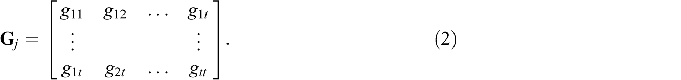
There are two levels of random effects in the models, one for teachers and the other for students. To calculate both of these in SAS PROC MIXED, which will be used when all responses are continuous, we use the RANDOM statement for the teachers and the REPEATED statement for the students. In SAS PROC GLIMMIX, used for binary and categorical outcomes, two RANDOM statements are listed. The standard variance structures for the RANDOM statement such as compound symmetry do not allow a correlation among the random teacher effects, so we must define the structure explicitly. Consider the matrix $G_{j}$ in Equation 2 with $t = 2$ . There are three variance components of interest: $g_{11}$ , $g_{22}$ , and $g_{12}$ . Each block $G_{j}$ is the same, for $j = 1, \dots, m$ . In SAS PROC MIXED, this structure is achieved using the variance structure “type=LIN( $q_{g}$ )” in the RANDOM statement where $q_{g}$ is the number of estimated variance components in $G$ . For the general VAA model in Equation 3, $q_{g} = t (t + 1) / 2$ ; if $t = 2$ and $q_{g} = 3$ ,

G = g_{11} A_{11} + g_{22} A_{22} + g_{12} A_{12},

where

A_{i j} = b l o c k d i a g (Δ_{i j})

and where

Δ_{i j}

is the

t \times t

matrix with 1 in the (i, j) and (j, i) elements and 0 elsewhere. The

A

matrices can be input into SAS PROC MIXED or GLIMMIXED using the “ldata” command with either the full matrices or a dense form; code for creating the matrices is given in Appendix B. The user should verify that the estimated G matrix is positive definite.

Value Added in Calculus Instruction

We now apply the models to data from a large public university. The study includes students who entered the university between fall 2000 and fall 2003 and who took at least one of the courses Calculus with Analytic Geometry II or III. These semesters were chosen since entry in those semesters allows at least 5.5 years for degree completion. The study, as with any VAA model, requires the students be linked to a teacher for every class; Broatch (2009) described the steps taken to resolve inconsistencies and link the data sets.

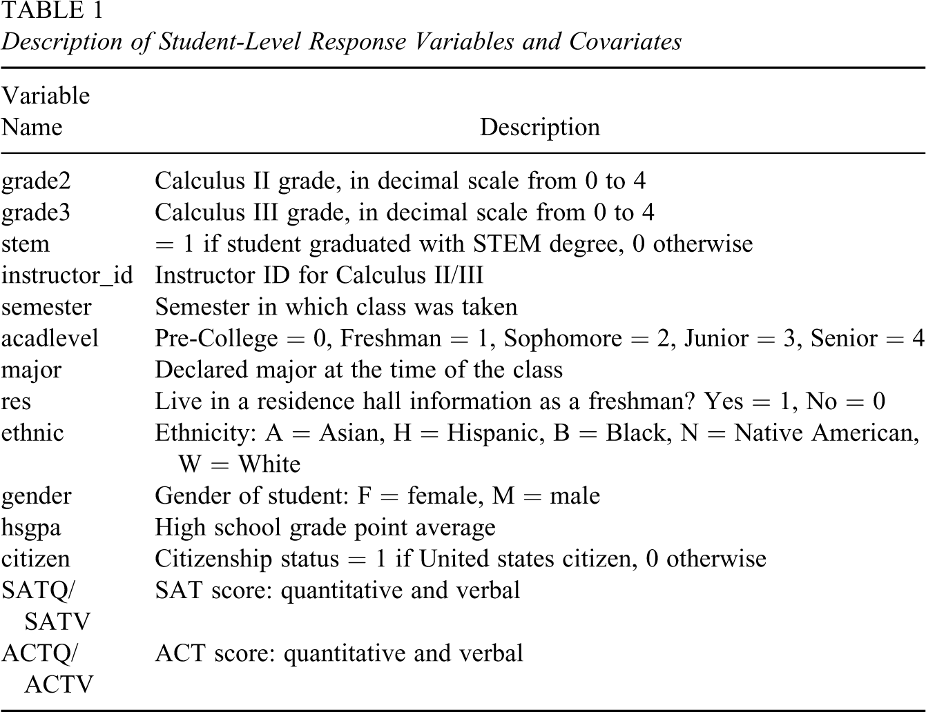
In this section, we present two models: (1) a model with both responses continuous, with $y_{i 1} =$ course grade in Calculus II for student $i$ and $y_{i 2} =$ course grade in Calculus III for student i, and (2) a model in which $y_{i 1} =$ course grade in Calculus III for student $i$ and $y_{i 2} = 1$ if student $i$ graduated with a STEM degree before fall 2009 and $y_{i 2} =$ 0 otherwise. Scores from a common final exam were unavailable, so course grade was used as a response indicating student achievement in the course. Tables 1 and 2list the response variables and covariates available for the analysis.

Table 1.

Description of Student-Level Response Variables and Covariates

Variable Name	Description
grade2	Calculus II grade, in decimal scale from 0 to 4
grade3	Calculus III grade, in decimal scale from 0 to 4
stem	= 1 if student graduated with STEM degree, 0 otherwise
instructor_id	Instructor ID for Calculus II/III
semester	Semester in which class was taken
acadlevel	Pre-College = 0, Freshman = 1, Sophomore = 2, Junior = 3, Senior = 4
major	Declared major at the time of the class
res	Live in a residence hall information as a freshman? Yes = 1, No = 0
ethnic	Ethnicity: A = Asian, H = Hispanic, B = Black, N = Native American, W = White
gender	Gender of student: F = female, M = male
hsgpa	High school grade point average
citizen	Citizenship status = 1 if United states citizen, 0 otherwise
SATQ/SATV	SAT score: quantitative and verbal
ACTQ/ACTV	ACT score: quantitative and verbal

Table 2.

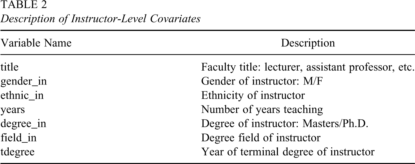
Description of Instructor-Level Covariates

Variable Name	Description
title	Faculty title: lecturer, assistant professor, etc.
gender_in	Gender of instructor: M/F
ethnic_in	Ethnicity of instructor
years	Number of years teaching
degree_in	Degree of instructor: Masters/Ph.D.
field_in	Degree field of instructor
tdegree	Year of terminal degree of instructor

For the first analysis with responses grade2 and grade3, only 24 instructors who taught both Calculus II and Calculus III were considered because of memory restrictions. The student information from the 2,051 students of those 24 teachers was then retained. Not all students took both classes at the university; many students take Calculus II in high school, while others do not continue on to Calculus III after taking Calculus II; thus, the data set used for the analysis had missing values. The model in Equation 3 may be fit to a data set with incomplete responses, making use of the available data for students with only one response. The model accounts for the missing data in three ways: through the covariance of the response in R, through the dependence with other students of that teacher, and through student covariates in X. While the multivariate approach presented in this paper allows inclusion of data from students with only one response and thus reduces potential bias that might result if their data were completely excluded, it does not explicitly model the missing data mechanism. McCaffrey and Lockwood (2011) studied pattern-mixture and selection models for missing data in VAA models and found that the estimates of teacher effects appear to be relatively robust to missing data assumptions.

Table 3presents the estimates of the fixed effects in the continuous model, omitting covariates that were not significant. No teacher covariates were significant in any of the models we fit. The covariate SATQ was significant, but it was not included since the covariate was missing for a large number of observations. Gender was also not significant in the full model, although it was significant in a model with no other covariates; in the full model, the covariate hsgpa explained the variability that otherwise would be explained by gender because female students have higher high school grade point averages. We also tested the null hypothesis that the slopes are the same for the two responses: Citizen is the only covariate with a significant difference between the grade2 parameter and the grade3 parameter ( $p - v a l u e = .0495$ ). Residual diagnostics using the marginal and conditional residuals revealed no patterns or other evidence of model inadequacy.

Table 3.

Fixed Effects Estimates and Standard Errors in the Continuous Model

Covariate	grade2 Estimate	Standard Error	grade3 Estimate	Standard Error
Intercept	−1.89	0.31	−1.87	0.30
ethnic = A	0.12	0.11	0.07	0.10
ethnic = B	−0.52	0.20	− 0.46	0.18
ethnic = H	−0.02	0.09	−0.04	0.09
ethnic = N	−0.83	0.20	−0.72	0.17
citizen	− 0.04	0.15	− 0.39	0.14
hsgpa	1.18	0.07	1.25	0.07
res	0.08	0.06	0.19	0.06

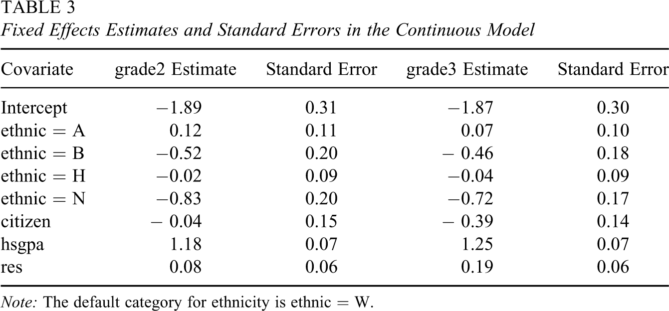
Note: The default category for ethnicity is ethnic = W.

The estimated covariance parameters for the model are

{\hat{G}}_{j} = [\begin{matrix} 0.21 (0.07) & 0.12 (0.05) \\ 0.12 (0.05) & 0.11 (0.04) \end{matrix}] a n d {\hat{R}}_{i} = [\begin{matrix} 1.45 (0.05) & 0.72 (0.06) \\ 0.72 (0.06) & 1.27 (0.05) \end{matrix}],

where the standard errors are provided in parentheses. For each response, the variance component due to the students is much larger than the variance component due to the teachers. The correlation between the effects is also high at both levels:

r_{G} = .80

and

r_{R} = .53

. Figure 1shows the bivariate predicted random teacher effects for the model with responses grade2 and grade3.

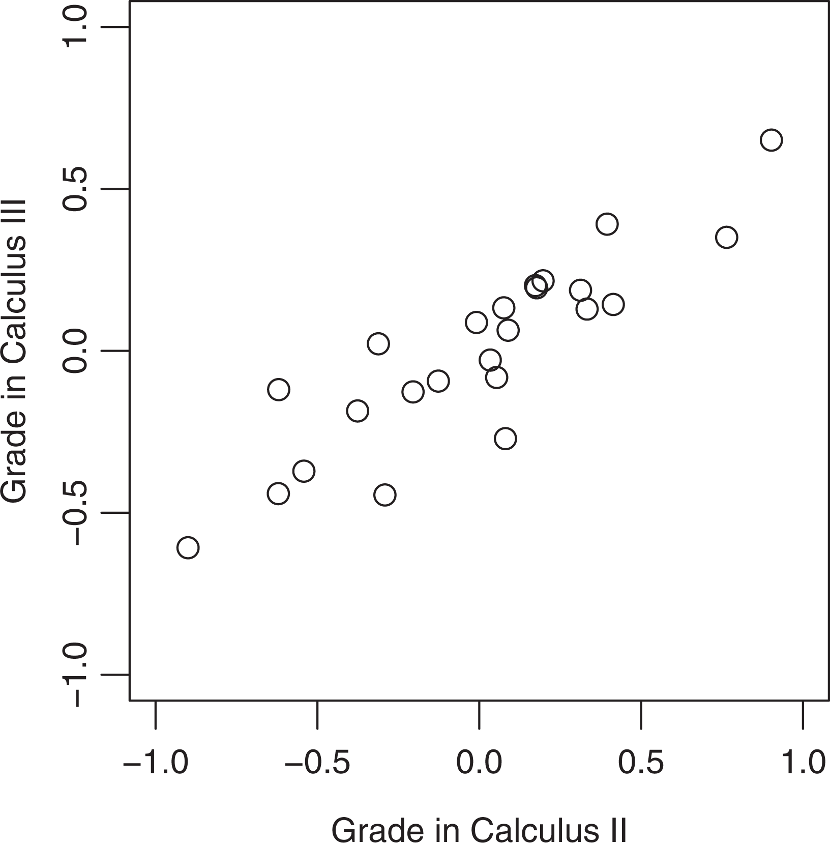
Predicted random teacher effects for responses of grades in Calculus II/III.

A likelihood ratio test of $H_{0} : g_{11} = g_{22}$ resulted in $X_{L R}^{2} = 3.7$ with $p$ -value of .054. The covariance term for the teachers, $g_{12}$ , is significantly different from 0 ( $X_{L R}^{2} = 14.1$ , $p$ -value = .0002). The hypothesis that $g_{11} = g_{22}$ is reasonable in this analysis since the responses are essentially the same variable measured for different classes.

The second analysis jointly models a continuous and binary response, with $y_{i 1}$ the value of grade3 and $y_{i 2}$ the value of stem. Again, different link functions can be used to allow for a variety of responses so the method is not limited to continuous and binary responses. Because the scale parameter for individuals is not identifiable with a binary response, we set $r_{22} = 1$ . See Rabe-Hesketh and Skrondal (2001) for a general discussion of identifiability in probit-normal models. We included all 54 Calculus III instructors in the data set for this analysis, along with the 3,407 students who took Calculus III. Table 4displays the estimates of the fixed effects, which are similar in direction to those in Table 3. The coefficients are not exactly the same for response grade3, however, because a larger data set was available for the second analysis.

Table 4.

Fixed Effects Estimates and Standard Errors in the Model With Responses stem and grade3

Covariate	grade3 Estimate	Standard Error	stem Estimate	Standard Error
Intercept	−1.47	0.21	−1.17	0.23
ethnic = A	−0.02	0.07	0.15	0.08
ethnic = B	−0.60	0.13	−0.32	0.14
ethnic = H	−0.17	0.06	−0.11	0.07
ethnic = N	−0.68	0.20	−0.63	0.14
citizen	−0.28	0.09	−0.14	0.11
hsgpa	1.12	0.05	0.39	0.06
res	0.11	0.04	0.04	0.05

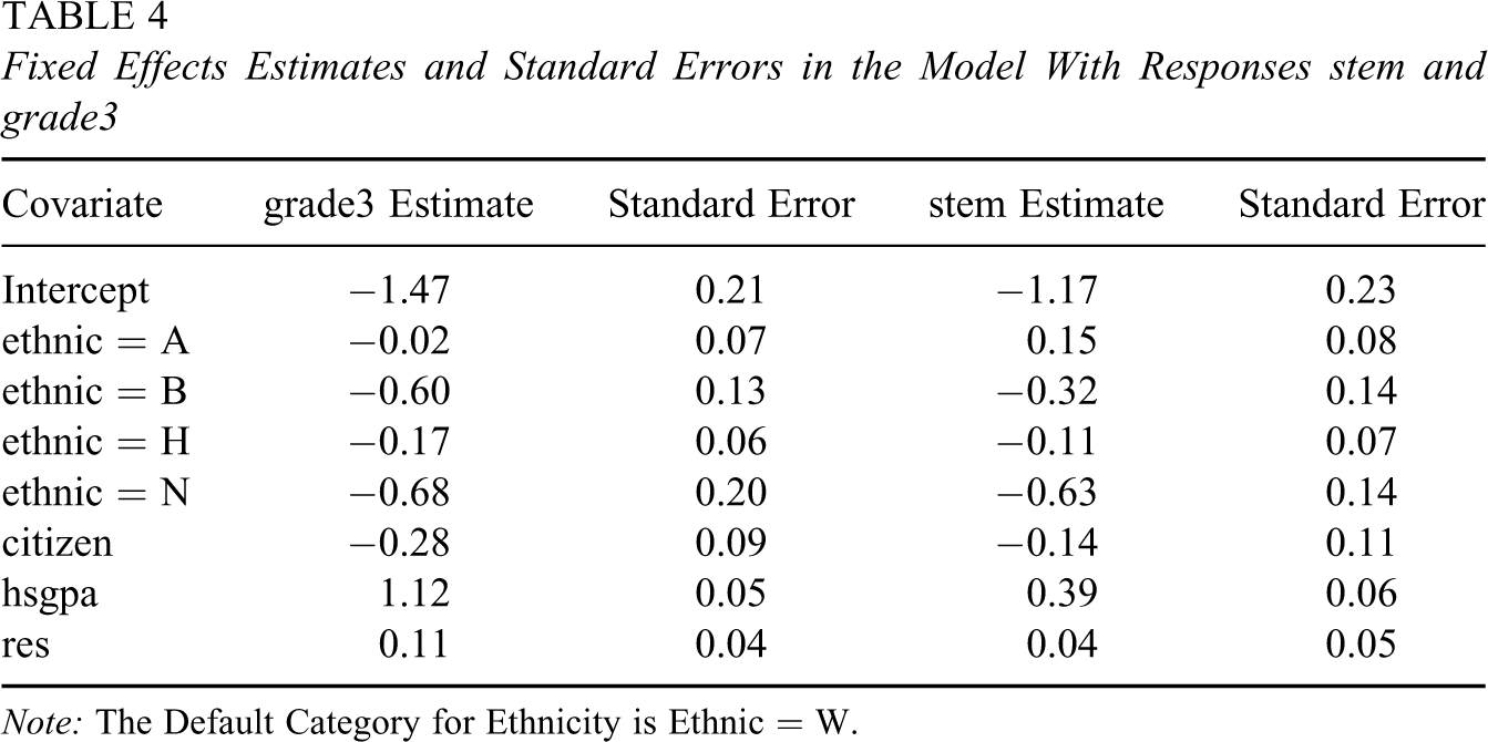
Note: The Default Category for Ethnicity is Ethnic = W.

The estimated covariance parameters for the model with responses grade3 and stem are:

{\hat{G}}_{j} = [\begin{matrix} \begin{matrix} 0.11 & (0.03) & - 0.04 & (0.02) \end{matrix} \\ \begin{matrix} - 0.04 & (0.02) & 0.09 & (0.03) \end{matrix} \end{matrix}] and {\hat{R}}_{i} = [\begin{matrix} \begin{matrix} 1.27 & (0.03) & 0.33 & (0.02) \end{matrix} \\ \begin{matrix} 0.33 & (0.02) & 1.00 & (- -) \end{matrix} \end{matrix}],

where the standard errors are provided in parentheses. Since the two responses are measured on different scales, the choices for G are limited. The models must include separate

g_{11}

and

g_{22}

parameters. Because the model was fit using pseudo-likelihoods, a likelihood ratio test cannot be used to test whether

g_{12} = 0

. The Wald test indicates that

g_{12}

is marginally significant at the .05 level.

Again, the variance components due to the students are substantially larger than the variance components due to the teachers, and the correlations of the student responses and teacher effects appear to be necessary in the model. The correlation within students for the responses is positive ( $r_{R} = .30$ ) as expected; one would expect students who receive higher grades in calculus to be more likely to graduate with a STEM degree. The unexpected result is that while $r_{R} > 0$ , the correlation between responses for the random teacher effects is negative ( $r_{G} = - .38$ ). Figure 2, displaying the bivariate predicted random teacher effects for the model with responses grade3 and stem, illustrates this negative correlation. Teachers with the largest positive effect for grade3 have the largest negative effect for stem. The estimated random effects for the teachers are therefore measuring very different aspects of their contributions to student outcomes. Because of the observational nature of the data set, we cannot say why this phenomenon occurs. Grade inflation is one possible explanation. It is possible that some teachers who give higher grades may be less inspiring so their students decide not to pursue a STEM degree. Alternatively, since students select their classes and instructors, students who do not intend to go on in mathematics and science may seek out instructors who have reputations for giving high grades. More information would be needed to be able to distinguish among various causal hypotheses for this phenomenon.

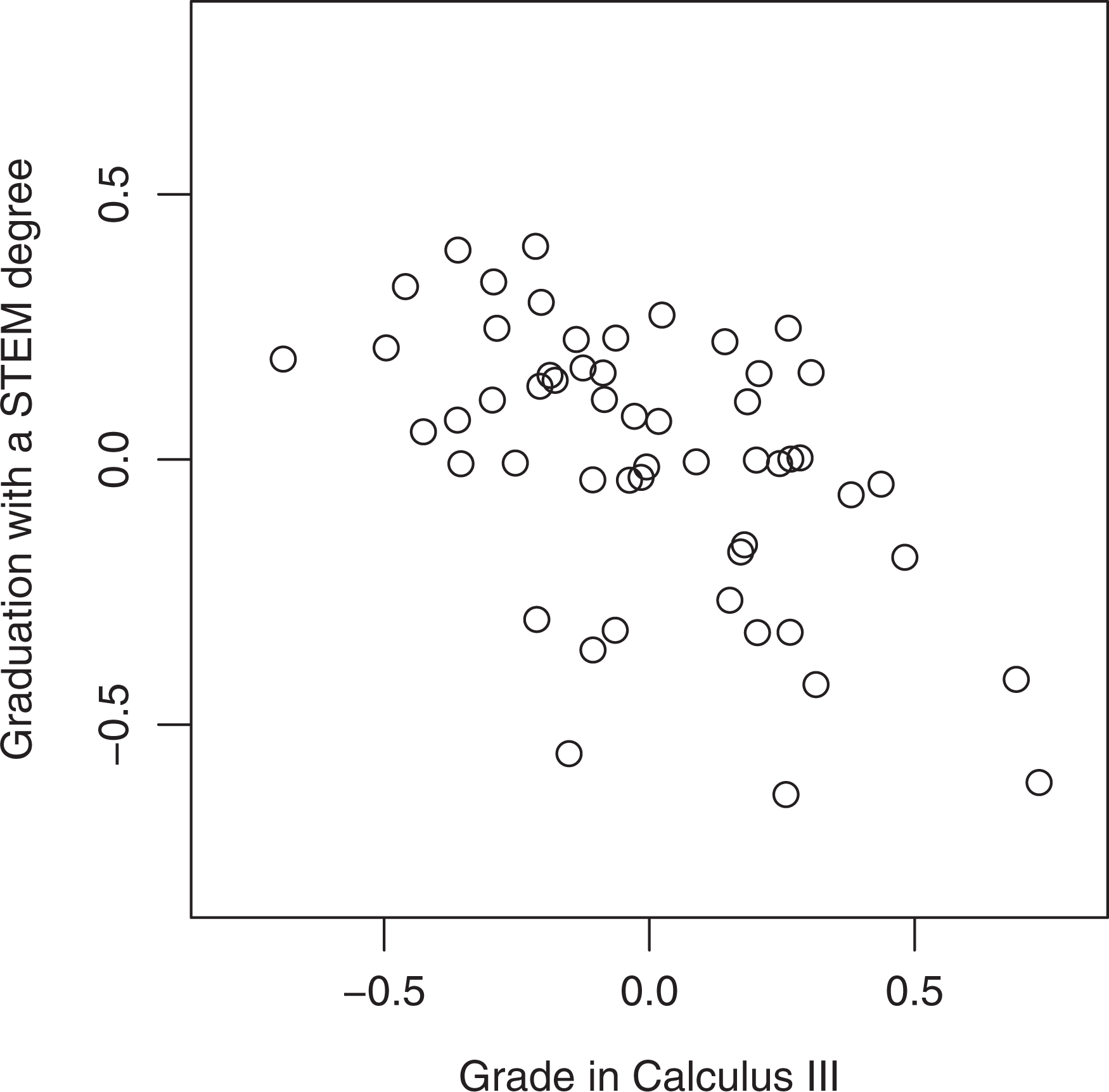
Predicted random teacher effects for responses: Grade in Calculus III and graduation with a STEM degree.

The MVAA models clearly provide more information for these data than a univariate model would have. They allow use of partial information for students who do not have a complete bivariate response, thereby reducing bias in the estimates and giving more precision for parameter estimates. The significance of $g_{12}$ in both models indicates that the unstructured G is an important extension. This covariance component should be considered for relevance in all VAA models. The multivariate model also provides more insight into the nature of teacher contributions to student outcomes. In the model where both responses are course grades, the teacher effects for the two responses are strongly positively correlated, as would be expected. But for the model with responses grade3 and stem, the correlation of the teacher effects for the two responses is small, but negative. In this case, grade3 and stem appear to be associated with two very different measures of teacher contributions.

Uses and Limitations of the MVAA Models

The model in Equation 3 includes random effects for teachers. If desired, a school level variable (third level of hierarchy) can be included similarly to the teacher effect. Also, a random factor for class nested within teacher can be included. Although the model makes explicit references to students, teachers, and time periods, the model can very easily be generalized to any two- or multilevel analysis with repeated measures. For example, you can model the effect of doctors (teachers) and hospitals (schools) on patients' (students') well-being over time. Regardless of the applied concept, the main goal is to be able to use the MVAA models to estimate the parameters of interest, that is, estimates of individual teacher and school effects and the overall contributions of the teachers to the variability of the student achievement.

When we have discussed this research with colleagues, the first question many people ask is which teachers are the best or worst, and who are the individual teachers appearing in Figures 1 and 2. Many researchers and policymakers argue that VAA models provide more information for teacher evaluation than some other approaches, and therefore should be an important component of official teacher evaluations. Gordon, Kane, and Staiger (2006) are among those who suggest using estimates from VAA models for decisions about hiring or firing teachers.

We believe that our results illustrate potential concerns about using estimates of individual teacher effects for ranking purposes. First, although the models can be used with data from randomized experiments, in most cases, they will be used with observational data. Unmeasured variables may have a large effect on the outcomes. We did not have information, for example, on the number of hours worked per week by the students; it is possible that students who work many hours would be concentrated in certain time slots. Since students choose which teacher they take, and since it is impossible to measure every factor in a student’s background that contributes to success, one cannot say that the estimate for a specific teacher is due to that teacher rather than to the characteristics of students who select that teacher.

Second, the results illustrate that potential rankings depend strongly on the particular outcome studied. Corcoran (2009) argued that if VAA model estimates are to be used for teacher assessment, at the very least they should be precise and consistent across outcomes measured. He also argued that they should admit a causal interpretation, which, given the observational nature of most data sets, does not occur. In our application, neither of Corcoran’s conditions is met. Figure 2 indicates a negative correlation between estimated teacher effects for one of the responses used in the evaluation of instructors at the university, namely, course grades, and a long-term outcome that is one of the stated goals of the university administration, namely, increasing the number of graduates in STEM fields. Thus, a ranking based on one of the responses will ignore contributions to the other response.

The MVAA models in this paper show the relationships among teacher contributions toward different student outcomes and allow consideration of binary real-world outcomes such as graduation or having a career in a STEM field. While they cannot capture the full complexity of student achievement, they can provide a much better picture than relying solely on univariate test scores.

Footnotes

Appendix A: Proof of Theorem 1

We show that the conditions in Theorem 2 of Mardia and Marshall (1984) hold, namely, that (a) the eigenvalues of $V$ and $V_{i}$ are bounded and (b) $| | V_{i} | |_{F}^{- 2} = O (n^{- 1 / 2 - δ})$ , for some $δ > 0$ for $i = 1, \dots, q$ , where $F$ denotes the Frobenius norm. Since $V = {S G S}^{'} + R$ , we have

\frac{\partial V}{\partial g_{i k}} = S Â b l o c k d i a g (Δ_{i k}) S^{'} a n d \frac{\partial V}{\partial r_{i k}} = b l o c k d i a g (Δ_{i k}),

where

Δ_{i k}

is the

t \times t

matrix with 1 in the

(i, k)

and

(k, i)

elements and 0 elsewhere. The second-order partial derivatives of

V

are all equal to zero so that the eigenvalues of the second-order partial derivative matrices are bounded.

We rely on properties of matrix norms to bound the eigenvalues of $V$ and $V_{i}$ . For an $n \times n$ symmetric matrix $A$ , $| | A | |_{2}$ is the maximum eigenvalue of A, and $| | A | |_{1} = max_{j} \sum_{i} | A_{i j} |$ . Let $g_{max}$ denote the maximum diagonal element of G. Since all elements of S are less than or equal to one,

| | S G S^{'} | |_{2} \leq | | S G S^{'} | |_{1} \leq {K t^{2} g}_{max}

. Similarly,

| | S b l o c k d i a g (Δ_{i k}) S^{'} | |_{2} \leq K t^{2} .

We now show condition (b). Let θ = g^ik. All elements of

S

and

Δ_{i k}

are greater than or equal to 0. Also, the

(j, j)

element of S′S is the number of students taking a particular class, which is assumed to be at least 1. Thus,

\begin{aligned} | | V_{ℓ} | |_{F}^{2} = | | S b l o c k d i a g (Δ_{i k}) S^{'} | |_{F}^{2} \\ = t r {S b l o c k d i a g (Δ_{i k}) S^{'} S b l o c k d i a g (Δ_{i k}) S^{'}} \\ \geq t r {I b l o c k d i a g (Δ_{i k}) I b l o c k d i a g (Δ_{i k})} \\ \geq m . \end{aligned}

Since the number of students in each class is bounded by

K, m \geq n / (K t),

so condition (b) is satisfied with

δ = 1 / 2.

Acknowledgments

This research was partially supported by the National Science Foundation under grants SES-0604373 and DRL-0909630. The authors thank the reviewers for their many helpful comments, which led to an improved paper.

Any opinions, findings, and conclusions or recommendations expressed in this material are those of the authors and do not necessarily reflect the views of the National Science Foundation or Arizona State University.

References

Ballou

Sanders

Wright

(2004). Controlling for student background in value-added assessment of teachers. Journal of Educational and Behavioral Statistics, 29, 37–65.

Berkhof

Snijders

T. A. B.

(2001). Variance component testing in multilevel models. Journal of Educational and Behavioral Statistics, 26, 133–152.

Breslow

N. E.

Clayton

D. G.

(1993). Approximate inference in generalized linear mixed models. Journal of the American Statistical Association, 88, 9–25.

Broatch

J. E.

(2009). Multivariate models for assessing educational effectiveness with continuous and categorical responses (Unpublished doctoral dissertation). Arizona State University

Corcoran

S. P.

(2009). “Value added” measures of teacher quality: Use and policy validity. Paper presented at the NYU Abu Dhabi Conference. Retrieved from https://steinhardt.nyu.edu/scmsAdmin/uploads/002/891/abudhabi2009SC.ppt

Demidenko

(2004). Mixed models: Theory and applications. Hoboken, NJ: Wiley.

Doran

H. C.

Lockwood

J. R.

(2006). Fitting value-added models in R. Journal of Educational and Behavorial Statistics, 31, 205–230.

Gelman

(2006). Prior distributions for variance parameters in hierarchical models. Bayesian Analysis, 1, 515–533.

Goldstein

Thomas

(1996). Using examination results as indicators of school and college performance. Journal of the Royal Statistical Society, Series A, 159, 149–163.

10.

Gordon

Kane

T. J.

Staiger

D. O.

(2006). Identifying effective teachers using performance on the job. Washington, DC: The Brookings Institution.

11.

Government Accountability Office. (2006). Science, technology, engineering, and mathematics trends and the role of federal programs (Tech. Rep. No. GAO-06-702T). Washington, DC: Author

12.

Hartley

H. O.

Rao

J. N. K.

(1967). Maximum-likelihood estimation for the mixed analysis of variance model. Biometrika, 54, 93–108.

13.

Lehmann

E. L.

(1999). Elements of large-sample theory. New York, NY: Springer.

14.

Lockwood

J. R.

McCaffrey

D. F.

Mariano

L. T.

Setodji

(2007). Bayesian methods for scalable multivariate value-added assessment. Journal of Educational and Behavioral Statistics, 32, 125–150.

15.

Mardia

K. V.

Marshall

R. J.

(1984). Maximum likelihood estimation of models for residual covariance in spatial regression. Biometrika, 71, 135–146.

16.

Mariano

L. T.

McCaffrey

D. F.

Lockwood

J. R.

(2010). A model for teacher effects from longitudinal data without assuming vertical scaling. Journal of Educational and Behavioral Statistics, 35, 253–279.

17.

Martineau

J. A.

(2006). Distorting value added: The use of longitudinal, vertically scaled student achievement data for growth-based, value-added accountability. Journal of Educational and Behavorial Statistics, 31, 35–62.

18.

McCaffrey

D. F.

Lockwood

J. R.

(2011). Missing data in value-added modeling of teacher effects. Annals of Applied Statistics. In press,

19.

McCaffrey

D. F.

Lockwood

J. R.

Koretz

D. M.

Hamilton

L. S.

(2003). Evaluating value-added models for teacher accountability. Santa Monica, CA: Rand Education.

20.

McCaffrey

D. F.

Lockwood

J. R.

Koretz

Louis

T. A.

Hamilton

L. S.

(2004). Models for value-added modeling of teacher effects. Journal of Educational and Behavioral Statistics, 29, 67–101.

21.

McCulloch

C. E.

(1994). Maximum likelihood variance components estimation for binary data. Journal of the American Statistical Association, 89, 330–335.

22.

Miller

J. J.

(1977). Asymptotic properties of maximum likelihood estimates in the mixed model of the analysis of variance. The Annals of Statistics, 5, 746–762.

23.

National Academy of Sciences. (2007). Rising above the gathering storm: Energizing and employing America for a brighter economic future. Washington, DC: National Academies Press.

24.

National Science Board. (2007). A national action plan for addressing the critical needs of the U.S. science, technology, engineering, and mathematics education system. Arlington, VA: National Science Foundation.

25.

Pinheiro

J. C.

Chao

E. C.

(2006). Effcient Laplacian and adaptive Gaussian quadrature algorithms for multilevel generalized linear mixed models. Journal of Computational and Graphical Statistics, 15, 58–81.

26.

Rabe-Hesketh

Skrondal

(2001). Parameterization of multivariate random effects models for categorical data. Biometrics, 57, 1256–1264.

27.

Raudenbush

S. W.

(2004). What are value-added models estimating and what does this imply for statistical practice?. Journal of Educational and Behavioral Statistics, 29, 121–129.

28.

Resnick

E. L. B.

(2004). Teachers matter: Evidence from value added assessments. Research Points, 2, 1–4.

29.

Rodríguez

Goldman

(2001). Improved estimation procedures for multilevel models with binary response: A case-study. Journal of the Royal Statistical Society. Series A, 164, 339–355.

30.

Rowan

Correnti

Miller

R. J.

(2002). What large-scale survey research tells us about teacher effects on student achievement: Insights from the Prospects study of elementary schools. Teachers College Record, 104, 1525–1567.

31.

Sanders

W. L.

Saxton

A. M.

Horn

S. P.

(1997). The Tennessee value-added multidimensional value added assessment 30 assessment system: A quantitative, outcomes-based approach to educational assessment. In Millman

(Ed.), Grading teachers, grading schools: Is student achievement a valid educational measure? (pp. 137–162). Thousand Oaks, CA: Corwin Press.

32.

SAS Institute Inc. (2008). SAS/STAT 9.2 user’s guide. Cary, NC: Author.

33.

Self

S. G.

Liang

K.-Y.

(1987). Asymptotic properties of maximum likelihood estimators and likelihood ratio tests under nonstandard conditions. Journal of the American Statistical Association, 82, 605–610.

34.

Tekwe

C. D.

Carter

R. L.

C.-X.

Algina

Lucas

M. E.

Roth

Ariet

Fisher

Resnick

M. B.

(2004). An empirical comparison of statistical models for value-added assessment of school performance. Journal of Educational and Behavioral Statistics, 29, 11–35.

35.

U.S. Department of Education. (2009). Students who study science, technology, engineering, and mathematics (STEM) in postsecondary education (Tech. Rep. No. NCES 2009–161). Washington, DC: Author

36.

Verbeke

Molenberghs

(2000). Linear mixed models for longitudinal data. Secaucus, NJ: Springer-Verlag.

37.

Wolfinger

O’Connell

(1993). Generalized linear mixed models: A pseudo-likelihood approach. Journal of Statistical Computation and Simulation, 48, 233–243.

38.

Wolfinger

Tobias

Sall

(1994). Computing Gaussian likelihoods and their derivatives for general linear mixed models. SIAM Journal on Scientific Computing, 15, 1294–1310.