The Generalized Multilevel Facets Model for Longitudinal Data

Abstract

In the human sciences, ability tests or psychological inventories are often repeatedly conducted to measure growth. Standard item response models do not take into account possible autocorrelation in longitudinal data. In this study, the authors propose an item response model to account for autocorrelation. The proposed three-level model consists of multiple facets (e.g., person, item, and rater facets) and slope parameters. Level 1 is an item response (within-occasion) model; Level 2 is a between-occasion and within-person model; and Level 3 is a between-person model. Parameters can be estimated using the computer software WinBUGS, which uses Markov Chain Monte Carlo (MCMC) algorithms. Through a series of simulations, it was found that the parameters in the proposed model can be recovered fairly well. Real data of job performance judged by raters at various time points were analyzed to illustrate the implications and application of the proposed model.

Keywords

item response theory longitudinal data autocorrelation multilevel models facets models Markov Chain Monte Carlo

In recent years, item response theory (IRT) has been widely applied to the social, behavioral, and health sciences. Most IRT models (e.g., the Rasch model, the two- and three-parameter logistic models and their polytomous extensions) are single-level. Consider a situation where we are interested in a group difference in a latent trait (e.g., gender difference in mathematics proficiency), or in using some background variables (e.g., age) to predict a latent trait. With single-level IRT models, the analysis consists of two stages. In Stage 1, an IRT model is fit to the data to obtain person measures. In Stage 2, an ordinary regression is applied to the person measures. The person measures are thus mistakenly treated as true values without measurement error. If the test was not sufficiently long and the measurement error is not trivial, then the results of the subsequent regression analysis can be seriously misleading. To resolve the problem of measurement error in person measures, one can form a two-level model in which Level 1 consists of an IRT model and Level 2 consists of a regression model. Since the criterion variable in the regression model is latent rather than observed, this approach is also called latent regression (Adams, Wilson, & Wu, 1997; Andersen, 2004; Christensen, Bjorner, Kreiner, & Petersen, 2004; Mislevy, 1985; Zwinderman, 1991).

Higher-level structures are possible. For instance, offspring can be grouped within families, and students can be nested within classes, which can be nested within schools. Offspring from a pair of parents tend to be more alike in their physical and mental characteristics than individuals chosen at random from the population at large. Students in a given class tend to be more homogenous than students who are randomly sampled from the population because the assignment of students to classes is not random but is based on geographic factors; students within a given class may come from a community with similar backgrounds, and they share a teacher, environment, and experiences.

Most IRT models consist of only two facets. That is, item responses are determined by an item facet and a person facet and the other factors are treated as random errors. In some testing situations, more than two facets may be involved; for example, item responses to essay items are often scored by raters and raters may hold different degrees of severity. Rater severity is often (if not always) too influential to be treated as a random noise. To better describe such kinds of data, several facets models have been proposed (Linacre, 1989, 2002; Lunz, Wright, & Linacre, 1990). In facets models, rater severity is often treated as a fixed effect, meaning that the rater holds a constant degree of severity throughout the rating process. This assumption may be too stringent in practice, because a rater may show a varying degree of severity during the rating process. Under such a case, it is more appropriate to treat rater severity as a random effect following a normal distribution. That is, each rater’s severity follows a distinct normal distribution, such that both intrarater and interrater variation in severity can be assessed. The random-effect facets model (Wang & Wilson, 2005) has such strength.

Advantages of multilevel IRT models include better reflection of a multilevel data structure, simultaneous estimation of item parameters and person measures, and accurate inference about higher-level measures (Fox, 2005; Kamata, 1998, 2001; Maier, 2001). Strengths of facets models consist of the simultaneous consideration of more than two facets in item responses so as to yield more accurate and valid measures (Linacre, 1989). Given that data may have a multilevel structure and more than two facets, it is natural to develop a generalized multilevel facets model, such as that recently proposed by Wang and Liu (2007).

Although the generalized multilevel facets model (Wang & Liu, 2007) is very general and includes many existing IRT models as special cases, it does not account for autocorrelation that is commonly found in repeated measures. Longitudinal data are commonly collected in the human sciences. For example, individuals are repeatedly measured on multiple occasions. The temporal ordering of the measurements is important because measurements closer in time within a person are likely to be more similar than observations farther apart in time. Longitudinal data have more statistical problems than cross-sectional data. Repeated observations on a given unit are seldom independent, and thus independence should be tested, not assumed. If the assumption of independence does not hold, the standard likelihood method of breaking up the likelihood of the sample into the product of individual likelihoods can no longer be applied. Stationarity is a basic assumption of longitudinal or time series analysis, which states that the choice of time origin does not affect the statistical properties of the process. When data do not meet this requirement, they can be transformed until they do through some stationary processes.

In the following empirical example, the data set requires complex IRT models to account for the rater effect, dependence in repeated observations, and latent regression. A set of workers from four departments of a company were evaluated by their managers on five criteria along a 5-point rating scale on four occasions. The item responses were ordinal and thus polytomous IRT models were needed. These IRT models should include a rater facet because the ratings were given by managers. The data were longitudinal and repeated observations of a given worker made by a manager may not be independent (e.g., carryover effects). Finally, workers in different departments might follow different growth trajectories, making latent regression necessary.

To meet this demand, we propose a multilevel facets model that can be applied to longitudinal data, show how to estimate its parameters, assess parameter recovery with a series of simulations, and demonstrate its application using an empirical example. This article is organized as follows. First, we introduce the simple Rasch model (1960) and its facets and multilevel extensions. Second, we propose a model which consists of three levels: a within-occasion item response model, a between occasion and within-person model, and a between-person model. Third, we explain how to use the Bayesian method of Markov Chain Monte Carlo (MCMC) to estimate parameters. Fourth, we describe a series of simulations that were conducted to assess parameter recovery and summarize the results. Finally, we provide a real data set of employees' job performances to demonstrate the application of the proposed model.

Facet Modeling

When person n responds to item i, the dichotomous Rasch model can be expressed as:

log i t (p_{n i 1}) \equiv log (p_{n i 1} / p_{n i 0}) = θ_{n} - b_{i},

(1)

where p_ni₁ and p_ni₀ are the probabilities of scoring 1 (i.e., y_ni = 1) and 0 (i.e., y_ni = 0) on item i for person n, respectively; and b_i is the difficulty of item i. Equation (1) contains two facets: item (b_i) and person (θ_n). When there are three facets (for example, when essay items are scored by raters), Equation (1) can be extended as:

log i t (p_{n i j k}) \equiv log (p_{n i j k} / p_{n i (j - 1) k}) = a_{i} [θ_{n} - (b_{i} + c_{i j}) - d_{k}],

where p_nijk and p_ni(j−1)kare the probabilities of scoring j and j–1 on item i for person n when judged by rater k, respectively; a_i is the discrimination parameter of item i; b_i is the overall difficulty of item i; c_ij is the jth threshold of item i relative to b_i; and d_k is the severity of rater k. To be general, Equation (2) has a discrimination parameter a_i. Models with more than three facets can be easily generalized.

Longitudinal Modeling

Equation (2) does not consider the possible dependence between repeated observations. To account for such dependence, we propose a generalized multilevel facets model for longitudinal data (denoted as GMFM-L), which consists of three levels. The Level 1 model describes item responses at a specific time point. The Level 2 model takes into account variation in the latent traits across measurement occasions within persons, in that a polynomial growth curve is specified to describe how the expected value of a response variable changes over time, and the covariance structure is autoregressive. The Level 3 model specifies the variation in growth trajectories between persons, which can be homoskedastic or heteroskedastic.

Level 1 Model

The Level 1 model describes item response functions, and is referred to as the item (or within-person) level. The log-odds of a response in category j over category j – 1 on item i for person n at time t when judged by rater k are formulated as:

log (p_{n t i j k} / p_{n t i (j - 1) k}) = a_{i} [θ_{n t} - (b_{i} + c_{i j}) - d_{n t k}],

(3)

where p_ntijk and p_nti(j−1)k are the probabilities of scoring j and j – 1, respectively, on item i for person n at time t when judged by rater k; θ_nt is the latent trait of person n at time t; d_ntk is the severity of rater k when judging person n at time t; and the others are defined as above. As suggested by Wang and Liu (2007), d_ntk is assumed to be a random effect following a normal distribution,

d_{n t k} \sim N (μ_{t k}, σ_{t k}^{2})

, where μ_tk describes the mean severity and

σ_{t k}^{2}

describes the intrarater variation in severity for rater k at time t. If the variance is zero, then the rater holds a constant degree of severity when judging persons (examinees) at that specific time point. A large variance suggests a large intrarater variation in severity. Interrater consistency can be assessed by a comparison of μ_tk across raters.

Note that in $d_{n t k} \sim N (μ_{t k}, σ_{t k}^{2})$ , a rater’s severity at time t is assumed to be independent of his or her severity at time t ′. This constraint of independence across time can be released by assuming that d_ntk follows a multivariate normal distribution with a nonzero covariance between time points for a rater. However, we do not pursue this complicated model in this study because of insufficient data points in the empirical example.

If there is only one time point (i.e., t = 1) and the rater holds an identical degree of severity for all persons (i.e., no intrarater variation), then Equation (3) reduces to Equation (2). For ease of estimation, one can specify the following normal priors for item parameters: $b_{i} \sim N (0, σ_{b}^{2})$ , $c_{i j} \sim N (0, σ_{c}^{2})$ , and $a_{i} \sim N (0, σ_{a}^{2})$ with the restriction a_i > 0. For model identification, the discrimination parameter a₁ and $\underset{j}{Σ} C_{i j}$ are fixed at 1 and 0, respectively.

Level 2 Model

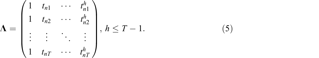
At Level 2, a latent growth model with an autoregressive residual structure is proposed as:

θ_{n t} = λ_{nt}^{'} η_{n} + ϵ_{n t},

(4)

where

η_{n}^{'} = [η_{n 0}, η_{n 1} \dots, η_{n h}]

is a vector of length h + 1 for the regression coefficients of person n,

λ_{n t}^{'} = [1, λ_{n t}^{1} \dots, λ_{n t}^{h}]

is a vector of time-based loadings (λ_nt is fixed at t_nt), and ϶_nt is a time-series residual. The time-based loading matrix Λ for a complete person is:

Λ = (\begin{matrix} 1 & t_{n 1} & \dots & t_{n 1}^{h} \\ 1 & t_{n 2} & \dots & t_{n 2}^{h} \\ ⋮ & ⋮ & ⋱ & ⋮ \\ 1 & t_{n T} & \dots & t_{n T}^{h} \end{matrix}), h \leq T - 1 .

(5)

For ϵ_nt, one can consider a second-order autoregressive residual model, abbreviated as AR(2):

ϵ_{n t} = ϕ_{1} ϵ_{n, t - 1} + ϕ_{2} ϵ_{n, t - 2} + z_{n t},

ϕ_{1} + ϕ_{2} < 1, ϕ_{2} - ϕ_{1} < 1, - 1 < ϕ_{2} < 1,

(6)

z_{n t} \sim N (0, σ_{z}^{2}),

where ϕ₁ and ϕ₂ are the autocorrelation parameters, and z_nt is a white noise series. Since the series is assumed to be stationary and ϶_n,t–1, ϶_n,t–2, …, and z_nt are assumed to be mutually independent, ϶_nt is normal with mean 0 and variance

σ_{ϵ}^{2}

(Appendix A).

For ease of estimation, one can specify normal priors for ϕ₁ and ϕ₂ as $ϕ_{1} \sim N (0, σ_{ϕ_{1}}^{2}) I (- 2, U_{1})$ and $ϕ_{2} \sim N (0, σ_{ϕ_{2}}^{2}) I (- 1, U_{2})$ with the restrictions that U₁ = 1 – ϕ₂ and U₂ = 1 + ϕ₁, where I (,) denotes a range within which sampling is confined. When ϕ₂ = 0, AR(2) reduces to AR(1). For AR(1), one can specify a uniform prior for ϕ as ϕ ∼ Unif (–1, 1). When ϕ₁ = ϕ₂ = 0, the distribution of ϵ_nt is white noise with mean 0 and variance $σ_{z}^{2}$ for all n and t.

Level 3 Model

In order to further describe variations in growth trajectories between persons, the Level 2 regression coefficients are regressed on another set of personal background variables:

η_{n} = γ_{n} ν + ς_{n},

(7)

ς_{n} \sim N (0, \sum_{ς}),

where γ_n is a set of observed predictors; is the regression parameters; and z_nt and σ_n are assumed to be mutually independent. If the variances of _n (with a length not larger than the number of time points) are constrained to be homogenous, then the model is homoskedastic; otherwise, it is heteroskedastic. To estimate the parameters within the Bayesian framework, one can specify a normal prior for and an inverse Wishart prior (or inverse Gamma prior when it is assumed that Σ_ς is a diagonal matrix) for Σ_ς (Segawa, 2005).

It can be shown that the GMFM-L consists of many standard IRT models as special cases. For example, when there is one time point, the GMFM-L reduces to the generalized multilevel facets model (Wang & Liu, 2007). Furthermore, if there are only two facets with a single time point and a single level, the GMFM-L reduces to the generalized partial credit model (GPCM; Muraki, 1992).

Parameter Estimation

The Bayesian approach is used for parameter estimation in the GMFM-L. In recent years, Bayesian methods have been widely applied to estimate parameters in complicated models, such as IRT models (Béguin & Glas, 2001; Patz & Junker, 1999a, 1999b), factor analysis models (Bartholomew, 1981; Lee, 1981), and structural equation models (Scheines, Hoijtink, & Boomsma, 1999). Implementing Bayesian analysis is both computationally intensive and cumbersome to program. Fortunately, the freeware WinBUGS provides users with a simple and user-friendly tool for performing Bayesian MCMC methods. There are various MCMC algorithms, including the Metropolis-Hastings algorithm (Hastings, 1970; Metropolis, Rosenbluth, Rosenbluth, Teller, & Teller, 1953) and the Gibbs sampling algorithm (Baker, 1998; Fox & Glas, 2001; Geman & Geman, 1984; Liu & Sabatti, 2000; Roberts & Smith, 1993).

The most prominent feature of the Gibbs sampling algorithm is that the underlying Markov Chain is constructed by composing a sequence of posterior distributions along a set of directions. In this study, data augmentation and the Gibbs sampling algorithm are used (Albert & Chib, 1993; Geman & Geman, 1984; Tanner, 1993; Tanner & Wong, 1987). Based on the data augmentation proposed by Tanner and Wong (1987), the observed data, y_obs, are augmented with the missing data y_mis = (θ, ), where θ is the latent trait and η is the regression coefficient. As a first step in the Bayesian approach, the prior distributions for all model parameters, denoted as δ, must be specified in order to form a posterior distribution. Denote the complete-data posterior as P(δ | y_mis, y_obs) = P(δ | y) and the observed-data posterior as P(δ | y _obs ). The posterior P (δ | y) is easier to handle than P(δ | y_obs) (Tanner & Wong, 1987; Zhang & Nesselroade, 2007). After augmenting the data, the general strategy underlying the Gibbs sampler is as follows:

1. Begin with an arbitrary starting point (δ⁽⁰⁾, θ⁽⁰⁾, η⁽⁰⁾).

2. Sample each parameter from its posterior distribution, conditioned on the previous values sampled for other parameters:

δ^{(1)} f r o m P (δ | θ^{(0)}, η^{(0)}, y_{o b s})

θ^{(1)} f r o m P (θ | δ^{(1)}, η^{(0)}, y_{o b s})

η^{(1)} f r o m P (η | δ^{(1)}, θ^{(1)}, y_{o b s})

…

δ^{(s)} f r o m P (δ | θ^{(s - 1)}, η^{(s - 1)}, y_{o b s})

θ^{(s)} f r o m P (θ | δ^{(s)}, η^{(s - 1)}, y_{o b s})

η^{(s)} f r o m P (η | δ^{(s)}, θ^{(s)}, y_{o b s})

In iteration s, parameters are sampled from their posteriors, conditioned on the parameters from iteration s – 1.

3. Continue this iterative process until a large number of samples are generated.

WinBUGS makes the Gibbs sampling algorithm easily accessible because users do not have to derive the full conditional distributions, and programming MCMC methods in WinBUGS is much easier than that in other computer languages (Segawa, 2005).

Deviance Information Criterion

The deviance information criterion (DIC; Spiegelhalter, Best, Carlin, & Linde, 2002) is defined as a Bayesian measure of model–data fit:

D I C = 2 E_{δ | y} (D (δ)) - D (E_{δ | y} (δ)),

E_{δ | y} (D (δ)) \approx \bar{D},

(8)

D (E_{δ | y} (δ)) \approx D (\bar{δ}),

D I C = 2 P D + D (\bar{δ}) = P D + \bar{D},

where

P D = \bar{D} - D (\bar{δ})

. A smaller DIC suggests a better model. To compute the DIC, we need to first carry out the burn-in. The average of the posterior samples of δ is calculated to produce an expected value of δ.

Model Comparison

A common approach for model comparison within the Bayesian framework is to compute a Bayes factor (Gelfand, 1996). When both models have an equal prior likelihood, the Bayes factor is defined as:

B F_{12} = f (y | M 1) / f (y | M 2),

(9)

where f (y | M1) and f (y | M2) are the marginal likelihood of the data matrix y for Model 1 and Model 2, respectively. A discussion of cross-validation principles in Bayes regression model selection was given by Geisser and Eddy (1979). In general, cross-validation methods involve predictions of a subset y_r of cases when only the complement of y_r, denoted as y_–r, is used to update the prior distribution of model parameters δ. The cross-validation predictions have the form:

f (y_{r} | y_{- r}) = \int f (y_{r} | δ, y_{- r}) π (δ | y_{- r}) d δ,

(10)

with f (y_r | y_–r) often referred to as the conditional predictive ordinate and π (δ | y_–r) often referred to as the posterior density (Congdon, 2003). Then, Equation (9) can be derived from Equation (10):

B F_{12} = f (y_{r} | y_{- r}, M 1) / f (y_{r} | y_{- r}, M 2) .

(11)

M1 is supported when BF₁₂ > 1, and M2 is supported otherwise. A value of BF₁₂ between 1 and 3 is considered as minimal evidence for M1, a value between 3 and 12 as positive evidence for M1, a value between 12 and 150 as strong evidence for M1, and a value greater than 150 as very strong evidence (Raftery, 1996). For computational convenience, the log of the Bayes factor in Equation (11), log (BF), is estimated as the difference between the marginal cross-validation log-likelihoods computed for Models 1 and 2.

The Simulation

Design

A series of simulations were conducted to examine parameter recovery and model–data fit of a two-level GMFM-L with an AR(2) structure and a linear growth curve. The simulated data sets contained four time points, each with the same two 7-point items. There were two groups of test-takers (persons), each with 120 persons. Each person’s item responses were scored by 4 of a total of 16 raters. The rater severity at the four time points was manipulated as follows. At t1 and t2, every rater had a severity generated from the given normal distribution N (0, 0.5); in other words, all raters had the same mean and variance of severity. At t3 and t4, the raters had severities generated from normal distributions with various means and variances.

The data were simulated as follows. First, the white noise series was randomly generated from the normal distribution N (0, 0.78). Second, the series values and the specified parameters (i.e., discrimination, difficulty, step, severity, time covariate, regression, and autocorrelation, shown in Table 2as true values) were used to calculate the corresponding category probability and the cumulative probabilities using Equation (3). Third, these cumulative probabilities were compared to a random number from a uniform (0, 1) distribution. The response was set at the category with the lowest cumulative probability larger than the random number.

Table 1.

Model Comparisons With the DIC and Cross-Validation Log-Likelihoods for Simulated and Real Data

Model	Feature	DIC	Cross-Validation Log-Likelihood
Simulated data
M1	$d_{n t k} \sim N (μ_{t k}, σ_{t k}^{2})$ , AR(2), step difficulty, two levels, linear	9969.38	−12411.72
M2	$d_{n k} \sim N (μ_{k}, σ_{k}^{2})$ , AR(2), step difficulty, two levels, linear	10341.79	−12586.79
M3	$d_{n k} \sim N (μ_{k}, σ_{k}^{2})$ , white noise, step difficulty, two levels, linear	10400.73	−12701.16
M4	Fixed effect, white noise, step difficulty, two levels, linear	15935.80	−25738.63
M5	Fixed effect, white noise, two levels, linear	23162.09	−43244.32
Real data
M6	GPCM, one level	47651.8	−22513.44
M7	$d_{n t k} \sim N (μ_{t k}, σ_{t k}^{2})$ , white noise, step difficulty, two levels, quadratic	47568.5	−22483.19
M8	$d_{n t k} \sim N (μ_{t k}, σ_{t k}^{2})$ , AR(1), step difficulty, two levels, quadratic	47453.4	−22463.47
M9	$d_{n t k} \sim N (μ_{t k}, σ_{t k}^{2})$ , AR(2), step difficulty, two levels, quadratic	47858.6	−22552.68
M10	$d_{n t k} \sim N (μ_{t k}, σ_{t k}^{2})$ , white noise, step difficulty, homoskedastic, three levels, quadratic	47569.1	−22498.98
M11	$d_{n t k} \sim N (μ_{t k}, σ_{t k}^{2})$ , white noise, step difficulty, heteroskedastic, three levels, quadratic	47702.1	−22524.65

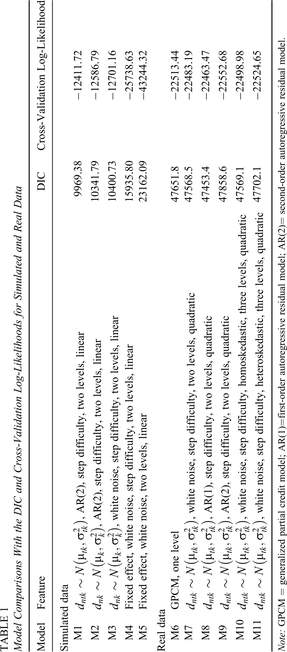
Note: GPCM = generalized partial credit model; AR(1)=first-order autoregressive residual model; AR(2)= second-order autoregressive residual model.

Table 2.

Bias and RMSE in Model 1 for Simulated Data

	Discrimination			Difficulty			Step 1			Step 2
Item	True	Bias	RMSE	True	Bias	RMSE	True	Bias	RMSE	True	Bias	RMSE
1	1^*			−0.64	0.014	0.282	−4.42	−0.005	0.061	−3.24	−0.008	0.035
2	4.56	−0.039	0.187	0.64	0.014	0.282	−4.56	0.058	0.091	−2.84	−0.056	0.072
	Step 3			Step 4			Step 5			Step 6
Item	True	Bias	RMSE	True	Bias	RMSE	True	Bias	RMSE	True	Bias	RMSE
1	−1.52	−0.002	0.011	2.16	0.016	0.023	2.45	0.017	0.039	4.56	−0.007	0.054
2	−0.98	0.000	0.013	1.52	−0.011	0.027	2.62	0.023	0.040	4.24	0.014	0.064
	Mean severity
Rater	Time 1			Time 2			Time 3			Time 4
	True	Bias	RMSE	True	Bias	RMSE	True	Bias	RMSE	True	Bias	RMSE
1	0.00	0.011	0.041	0.00	−0.002	0.041	−0.06	−0.013	0.021	0.04	0.016	0.024
2	0.00	−0.003	0.029	0.00	−0.010	0.040	0.02	−0.010	0.024	0.14	−0.020	0.027
3	0.00	0.020	0.041	0.00	−0.008	0.030	−0.78	0.008	0.019	−1.04	−0.008	0.020
4	0.00	0.001	0.037	0.00	0.011	0.033	−0.48	0.006	0.016	−0.64	−0.010	0.019
5	0.00	−0.007	0.038	0.00	0.006	0.036	0.16	0.006	0.015	0.78	−0.016	0.026
6	0.00	−0.002	0.037	0.00	0.011	0.038	0.48	0.016	0.024	0.58	−0.024	0.036
7	0.00	0.006	0.035	0.00	−0.010	0.028	−0.12	−0.008	0.031	−0.08	0.024	0.031
8	0.00	−0.008	0.041	0.00	0.004	0.026	−0.48	−0.019	0.029	−0.48	0.016	0.046
	Mean severity
Rater	Time 1			Time 2			Time 3			Time 4
	True	Bias	RMSE	True	Bias	RMSE	True	Bias	RMSE	True	Bias	RMSE
9	0.00	−0.003	0.028	0.00	−0.004	0.030	0.42	0.003	0.037	−0.04	0.029	0.036
10	0.00	−0.001	0.028	0.00	0.004	0.030	−0.02	−0.020	0.031	1.62	−0.022	0.041
11	0.00	−0.010	0.036	0.00	−0.010	0.035	−0.48	0.014	0.027	−0.18	0.010	0.025
12	0.00	0.005	0.041	0.00	0.001	0.027	1.24	−0.018	0.047	0.36	−0.004	0.033
13	0.00	0.002	0.040	0.00	0.004	0.042	0.28	0.004	0.015	−0.01	0.007	0.064
14	0.00	−0.011	0.028	0.00	0.019	0.051	0.54	−0.010	0.020	0.36	−0.017	0.035
15	0.00	0.000	0.041	0.00	−0.021	0.042	−0.06	0.030	0.035	−1.04	0.021	0.038
16	0.00	0.001	0.037	0.00	0.005	0.027	−0.66	0.012	0.025	−0.38	0.009	0.030
	Variance of severity
Rater	Time 1			Time 2			Time 3			Time 4
	True	Bias	RMSE	True	Bias	RMSE	True	Bias	RMSE	True	Bias	RMSE
1	0.5	−0.001	0.012	0.5	0.001	0.010	2.0	0.033	0.072	2.4	−0.002	0.070
2	0.5	−0.001	0.007	0.5	0.000	0.009	2.7	0.020	0.094	2.5	0.039	0.084
3	0.5	−0.001	0.009	0.5	−0.002	0.008	0.2	0.030	0.030	2.0	0.084	0.111
4	0.5	0.000	0.007	0.5	0.005	0.013	0.3	0.019	0.020	2.5	−0.092	0.112
5	0.5	0.002	0.008	0.5	−0.002	0.008	0.8	0.100	0.011	0.8	−0.011	0.036
6	0.5	−0.003	0.009	0.5	0.002	0.009	2.5	0.029	0.093	0.4	0.023	0.034
7	0.5	−0.002	0.012	0.5	0.001	0.009	3.4	−0.037	0.122	1.0	0.031	0.055
8	0.5	0.003	0.011	0.5	−0.001	0.007	1.4	0.012	0.060	3.8	−0.036	0.134
	Variance of severity
Rater	Time 1			Time 2			Time 3			Time 4
	True	Bias	RMSE	True	Bias	RMSE	True	Bias	RMSE	True	Bias	RMSE
9	0.5	−0.002	0.010	0.5	0.000	0.009	3.7	0.040	0.107	1.9	0.018	0.097
10	0.5	−0.002	0.011	0.5	0.000	0.006	0.5	0.064	0.082	1.2	−0.055	0.069
11	0.5	0.000	0.008	0.5	0.000	0.008	3.4	0.027	0.108	2.4	−0.023	0.071
12	0.5	0.001	0.010	0.5	−0.001	0.009	2.7	−0.031	0.078	2.2	−0.033	0.111
13	0.5	−0.001	0.009	0.5	0.001	0.009	3.2	−0.006	0.102	1.6	−0.012	0.060
14	0.5	0.000	0.007	0.5	−0.004	0.009	3.7	−0.013	0.137	6.2	0.081	0.212
15	0.5	0.000	0.010	0.5	−0.001	0.008	3.0	0.012	0.060	1.5	−0.016	0.065
16	0.5	0.001	0.008	0.5	0.002	0.009	2.5	−0.035	0.068	2.8	−0.044	0.087
Regression group	Intercept			Linear
Regression group	True	Bias	RMSE	True	Bias	RMSE
1	0.28	−0.019	0.695	−0.08	−0.021	0.519
2	0.18	−0.014	0.686	0.24	0.021	0.520
Autocorrelation	True	Bias	RMSE
First-order	0.04	0.000	0.010
Second-order	0.06	0.003	0.494
White noise variance	0.78	0.008	0.157

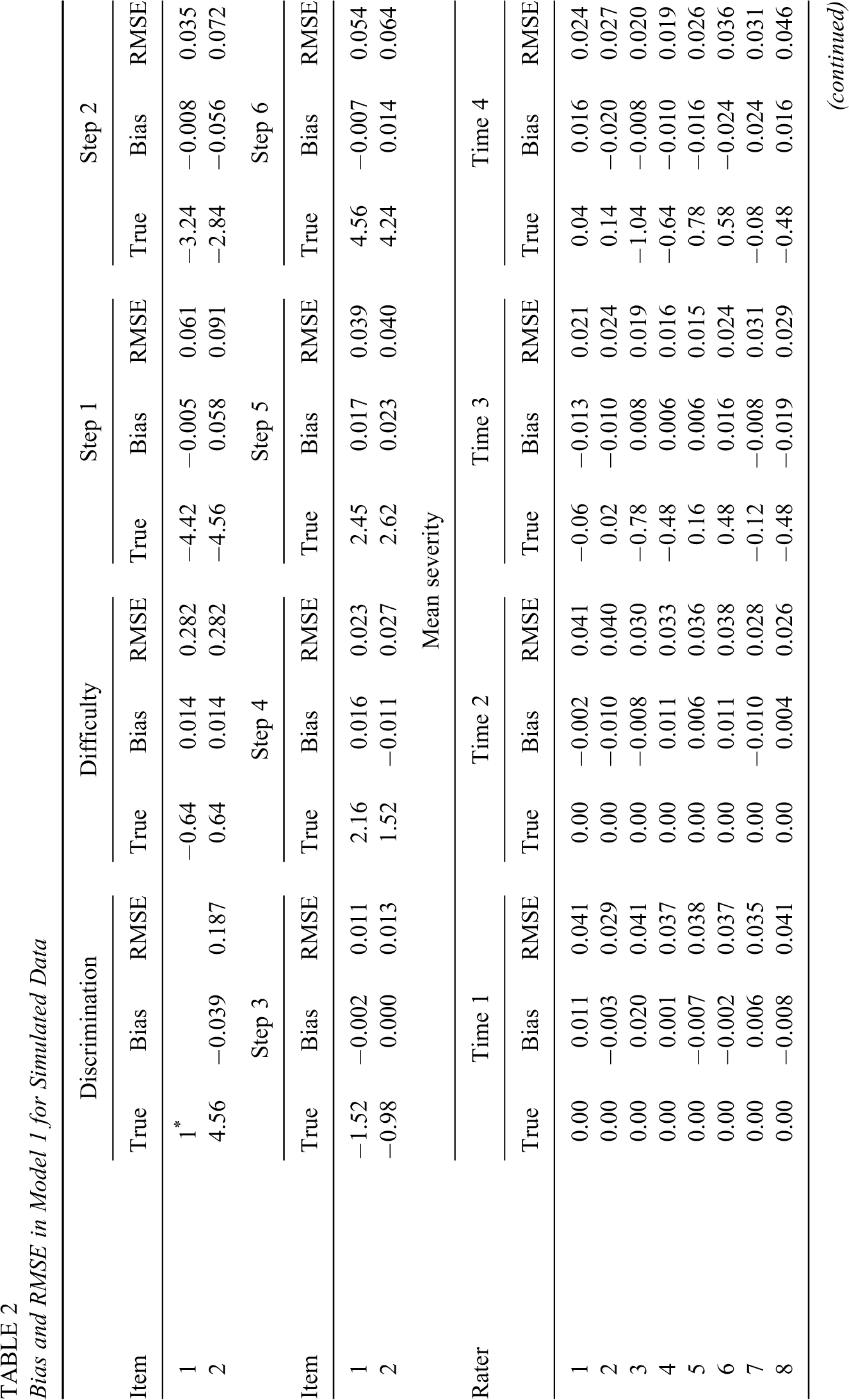
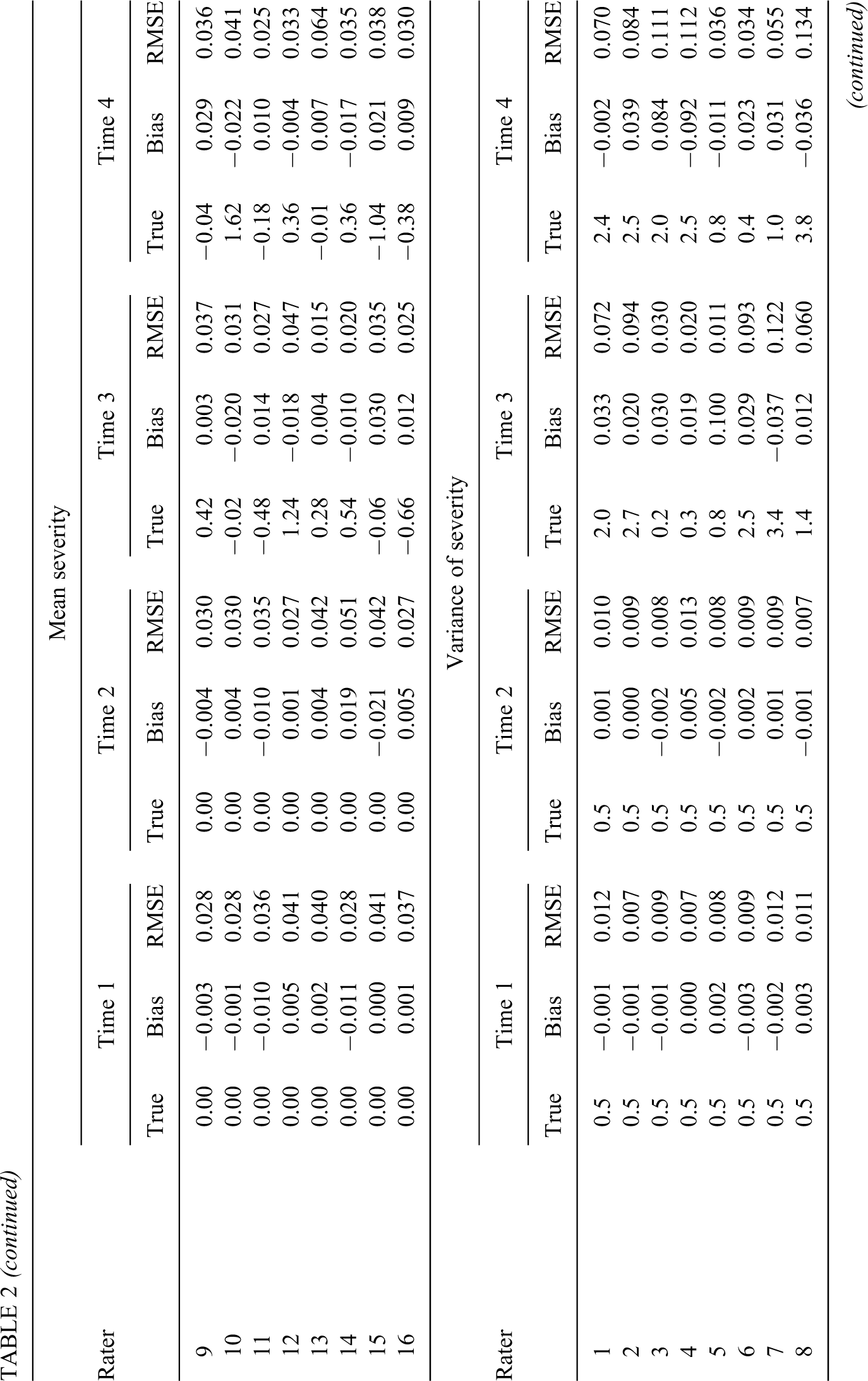
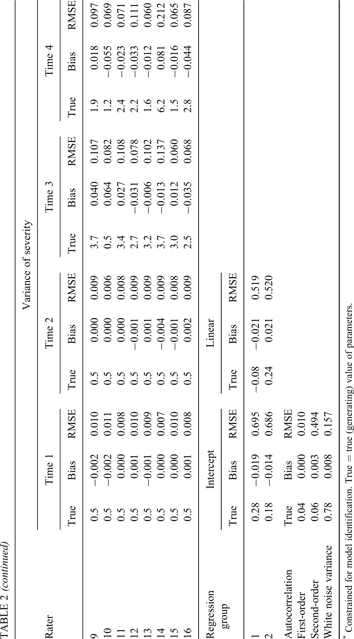
^* Constrained for model identification. True = true (generating) value of parameters.

In the analysis, we were interested in the following effects on parameter estimation or model-data fit: (a) intrarater and interrater consistency: at t1 and t2 all raters had identical intrarater consistency and interrater consistency, at t3 and t4 all raters had different intrarater consistency and interrater consistency; (b) rater–time interaction: each rater had varying severity across time points or each rater had an identical severity across time points; (c) autoregressive residuals: white noise or AR(2); and (d) step difficulties over items: each item had a set of step difficulties (i.e., the partial credit modeling; Masters, 1982) or all items shared the same set of step difficulties (i.e., the rating scale modeling; Andrich, 1978).

After the item responses were generated, five models (M1 to M5) were fit using WinBUGS. The upper part of Table 1describes the features of the five models. A total of 30 replications were made. M1 was the generating model. M2 did not consider the time effect; that is, every rater was assumed to hold the same severity distribution across the four time points. M3 was formed by constraining the autocorrelation parameters of M2 to zero; the model became a white noise model. M4 was formed by further constraining the random effect of rater severity in M3 to a fixed effect where the variance of severity for every rater was set to zero. Finally, M5 was formed by constraining the step difficulties of M4 to be the same across items.

In this simulation, the priors were specified as:

ϕ_{1} \sim N (0, 1.0 E - 6) I (- 2, U_{1}),

ϕ_{2} \sim N (0, 1.0 E - 6) I (- 1, U_{2}),

a_{i} \sim N (0, 0.25) I (0,), i = 2, \dots, I;

b_{i} \sim N (0, 0.25), i = 1, \dots, I;

c_{i 1} \sim N (0, 0.04) I (, c_{i 2}), i = 1, \dots, I,

c_{i 2} \sim N (0, 0.04) I (c_{i 1}, c_{i 3}), i = 1, \dots, I,

…

c_{i 6} \sim N (0, 0.04) I (c_{i 5},), i = 1, \dots, I;

ν \sim N (0, 1.0 E - 5);

σ_{z}^{2} \sim I G (3, 1);

μ_{t k} \sim N (0, 0.25) {, σ}_{t k}^{2} \sim I G (3, 1), t = 1, \dots, T, k = 1, \dots, K .

A total of 8,000 iterations provided sufficient convergence. An additional 4,000 iterations were conducted to provide sampled parameter values for posterior summarization.

The “eyeball” method, monitoring the convergence by visually inspecting the history plots of the generated sequences, is commonly used. Usually, if there is no change point or trend in the plot, the convergence of the generated sequence is accepted (Zhang, Hamagami, Wang, Grimm, & Nesselroade, 2007, p. 377). To obtain accurate estimates, the Monte Carlo error for each parameter of interest should be smaller than 5% of the standard deviation (Spiegelhalter, Thomas, Best, & Lunn, 2003). Bias and root mean square error (RMSE) were used to assess parameter recovery.

Results

There were 149 parameters in the generating model M1, including 1 discrimination parameter for Item 2 (Item 1’s discrimination was constrained to be unity for model identification), 1 difficulty parameter for Item 2 (Item 1’s difficulty was constrained to be the negative value of Item 2’s difficulty for model identification), 6-step parameters for each item, 3 autocorrelation parameters (ϕ₁,ϕ₂, and $σ_{z}^{2}$ ), 4 regression parameters (η₀ and η₁ for each of the two groups of persons), 16 parameters for the mean severity at each of the four time points, and 16 parameters for the variance of severity at each of the four time points.

When the generating model (M1) was fit to the data, as shown in Table 2, it was found that the bias was –0.039 for the discrimination, 0.014 for the difficulty, –0.056 ∼ 0.058 for the step parameters, 0.000 ∼ 0.008 for the autocorrelations, –0.021 ∼ 0.021 for the regressions, –0.021∼ 0.020 for the mean severity of the first two time points, –0.024 ∼ 0.030 for the mean severity of the last two time points, –0.004 ∼ 0.005 for the variance of severity of the first two time points, and –0.092 ∼ 0.100 for the variance of severity of the last two time points. All but the variance of severity of the last two time points had a bias very close to zero. The RMSE was 0.187 for the discrimination, 0.282 for the difficulty, 0.011 ∼ 0.091 for the step parameters, 0.01 ∼ 0.494 for the autocorrelation parameters, 0.519 ∼ 0.695 for the regression parameters, 0.026 ∼ 0.051 for the mean severity of the first two time points, 0.015 ∼ 0.060 for the mean severity of the last two time points, 0.006 ∼ 0.013 for the variance of severity of the first two time points, and 0.011 ∼ 0.212 for the variance of severity of the last two time points. The RMSE for the last two time points (where different raters had different variances of severity) was larger than that for the first two time points (where all raters had a common variance of severity of 0.5), which might be due to the magnitude of the variances for the last time points (0.2 ∼ 6.2, M = 2.2) being larger than that for the first two time points. As also shown in Figure 1, ϕ₂ and the four regression parameters had a large RMSE (0.494 ∼ 0.695), which might be due to the small number of time points and insufficient replications.

Figure 1.

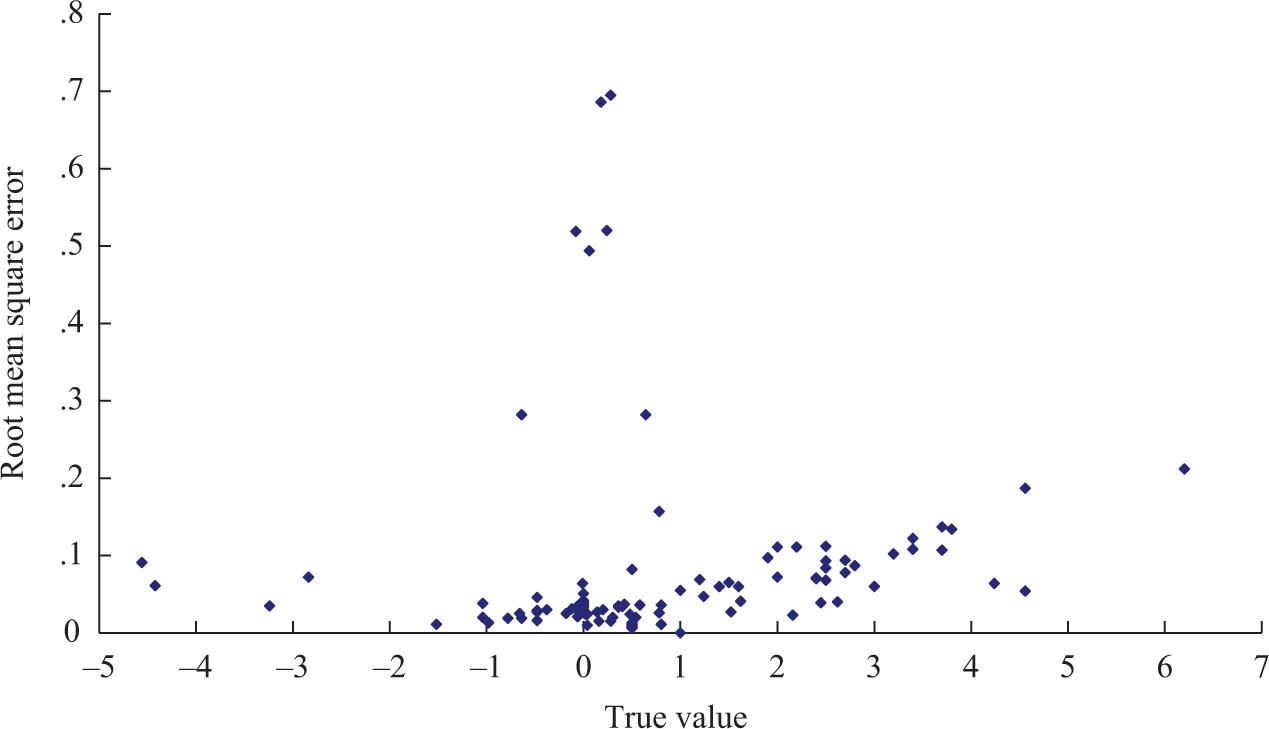
Root mean square error across true values when the generating model is fit.

M2 through M5 were also fit to the data. Since these models were nested and M1 was the most general (and the generating model) and M5 was the least general, it was expected that M1 would have the best fit and M5 would have the worst fit. According to the averaged DIC and the averaged cross-validation log-likelihood across 30 replications (shown in Table 1), as expected, M1 was the best-fitting model and M5 was the worst-fitting model. The difference in the averaged DIC was 372.41 between M1 and M2, 58.94 between M2 and M3, 5535.07 between M3 and M4, and 7226.29 between M4 and M5. The difference in the averaged cross-validation log-likelihood was 175.07 (which is equivalent to the log-BF) between M1 and M2, 114.37 between M2 and M3, 13037.50 between M3 and M4, and 17505.70 between M4 and M5. Relatively speaking, the constraint of a second-order autocorrelation as white noise and the constraint of a constant severity distribution across time were less harmful to model–data fit than the constraint of a common set of step parameters for all items and the constraint of no intrarater variation in severity.

An Empirical Example

A total of 238 workers from four departments of an electronic firm in Taiwan were assessed on four occasions (once per season) by five managers according to five job criteria (thoroughness, creativity, complexity, structure, and accuracy) along a 5-point rating scale. The higher the rating, the better the job performance is. Departments 1 through 4 had 54, 66, 60, and 58 workers, respectively.

We were interested in the following questions:

Was multilevel modeling necessary?

What kind of modeling for autocorrelation was more appropriate? White noise, AR(1), or AR(2)?

Were the growth trajectories homoskedastic or heteroskedastic?

What were the intrarater and interrater variations in severity?

To answer these four major questions, a set of six models was formed, denoted as M6 through M11, respectively. M6 was a single-level model, which is equivalent to that proposed by Wang and Liu (2007). M7, M8, and M9 were two-level models (criteria and occasions), with autoregressive residuals constrained as white noise, AR(1), and AR(2), respectively. M10 and M11 were three-level models (criteria, occasions, and workers) with a homoskedastic structure and a heteroskedastic structure, respectively. The larger the code of the model (e.g., M11), the more general the model is.

The lower part of Table 1 lists the DIC statistics and the cross-validation log-likelihoods for the six models. M8 was the best-fitting model (its WinBUGS commands are listed in Appendix B). Thus, two-level modeling was more appropriate than one-level and three-leveling modeling; first-order modeling was better than white noise and second-order modeling for the autoregressive residuals. Table 3lists parameter estimates of M8. The estimates for the item discrimination parameters were between 0.052 (accuracy) and 3.887 (creativity); those for the difficulty parameters were between –4.026 (accuracy) and 2.29 (creativity). Hence, creativity was not only the most important criterion of job performance but also the most difficult to achieve. Different items had very different step difficulties. For example, the step difficulties were –2.44 ∼ 2.525 for creativity but –12.46 ∼ 12.11 for accuracy. The huge variation in step difficulty across items was mainly due to the items having very different discrimination powers (0.052 ∼ 3.887). A quadratic growth curve was applicable to Department 1, $μ_{θ_{t}} = - 0.202 + 0.391 t + 0.066 t^{2}$ , but not to other departments. The first-order autocorrelation over time ϕ₁ was not trivial, with an estimate of –0.118, suggesting that a two-level structure had a better fit than that of a single-level structure. The estimate of white noise variance $σ_{z}^{2}$ was as high as 3.324, suggesting a large unexplained interperson variation.

Table 3.

Parameter Estimates and Standard Errors (in Parentheses) in Model 8 for Real Data

Item	Discrimination	Difficulty	Step 1	Step 2	Step 3	Step 4
1	1^*	0.125 (.405)	−2.465 (.144)	−1.598 (.083)	1.459 (.062)	2.605 (.097)
2	3.887 (.718)	2.290 (.392)	−2.440 (.103)	−1.133 (.054)	1.048 (.052)	2.525 (.092)
3	0.169 (.010)	0.843 (.680)	−5.180 (.446)	−4.562 (.329)	4.843 (.299)	4.898 (.300)
4	0.101 (.007)	0.768 (.949)	−8.580 (.838)	−7.481 (.679)	7.995 (.601)	8.066 (.605)
5	0.052 (.003)	−4.026 (1.109)	−12.460 (1.083)	−11.590 (1.006)	11.940 (.957)	12.110 (.970)
	Mean severity
Rater	Time 1	Time 2	Time 3	Time 4
1	−0.129 (.134)	0.136 (.142)	−0.296 (.119)	−0.100 (.132)
2	0.731 (.082)	0.504 (.091)	0.538 (.083)	0.625 (.100)
3	−0.306 (.130)	−0.646 (.164)	−0.461 (.154)	−0.583 (.154)
4	−0.853 (.155)	−0.446 (.202)	−0.175 (.124)	−0.533 (.153)
5	0.557 (.085)	0.450 (.089)	0.395 (.085)	0.591 (.097)
	Variance of severity
Rater	Time 1	Time 2	Time 3	Time 4
1	3.963 (.656)	3.789 (.628)	2.807 (.451)	3.370 (.597)
2	0.704 (.138)	0.603 (.115)	0.716 (.134)	0.868 (.180)
3	5.009 (.776)	5.862 (.951)	5.230 (.833)	5.204 (.917)
4	4.714 (.824)	6.150 (1.013)	4.273 (.663)	4.713 (.920)
5	0.882 (.168)	0.688 (.129)	0.709 (.140)	0.871 (.190)
Regression	Intercept	Linear	Quadratic
Dep. 1	−0.202 (.224)	0.391 (.202)	0.066 (.198)
Dep. 2	−0.059 (2.040)	0.005 (2.016)	0.001 (1.989)
Dep. 3	−0.002 (1.968)	0.028 (2.006)	−0.002 (1.894)
Dep. 4	0.149 (2.012)	−0.020 (2.022)	0.008 (1.903)
Autocorrelation
First-order	−0.118 (.040)
White noise variance	3.324 (.266)

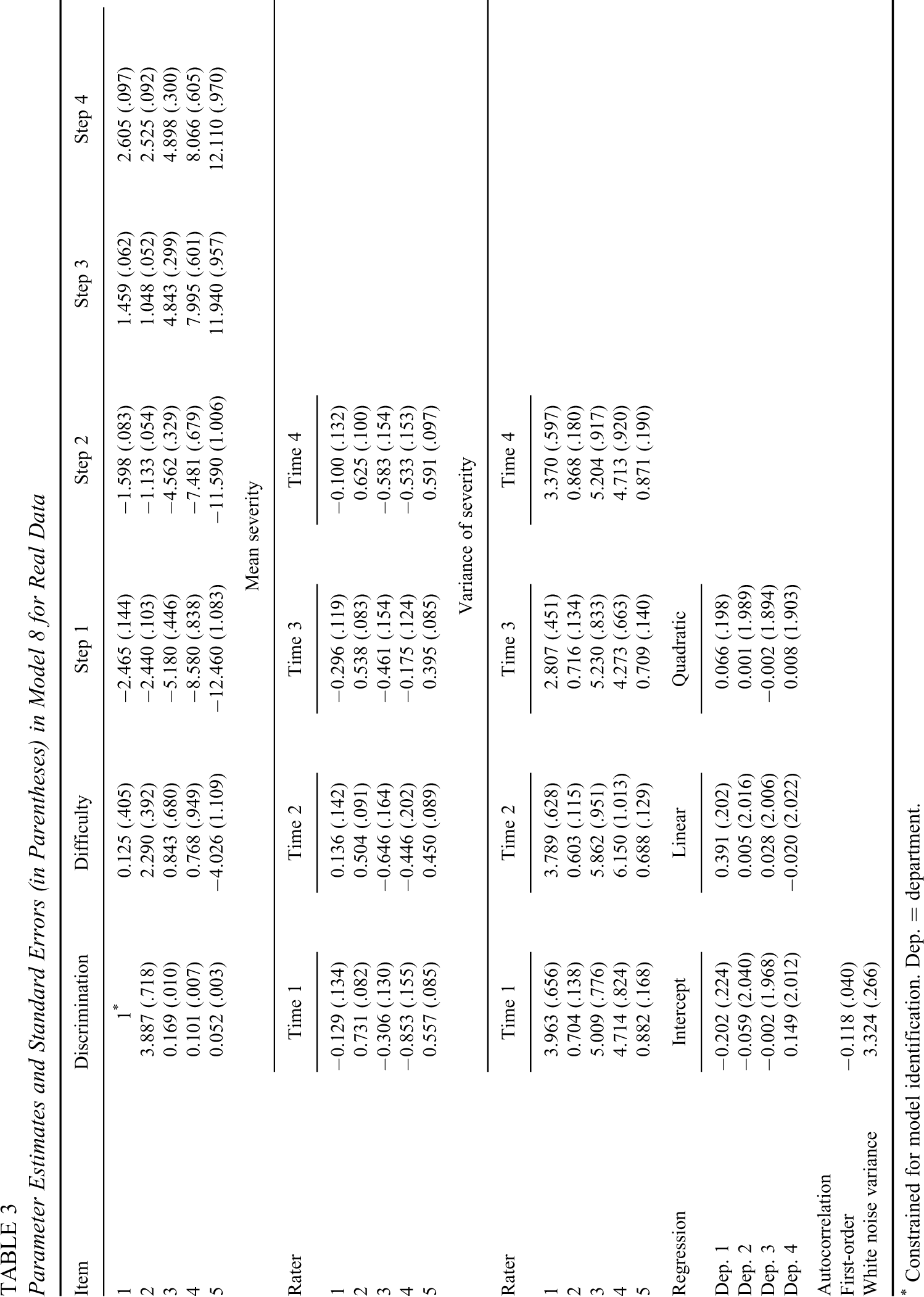
^* Constrained for model identification. Dep. = department.

In M8 as well as other models, each rater’s severity was assumed to follow a normal distribution. Figure 2 shows the mean severity of the five raters across time points. Raters 2 and 5 have larger mean severities (i.e., more severe) than those of the other three raters throughout the four time points. As the time point moved forward, the mean severities of the five raters became more similar. Figure 3 shows the variances of severity of the five raters across time points. Raters 2 and 5 have much smaller variances than those of the others, indicating that their intrarater variation in severity was smaller. Figures 2 and 3 reveal that compared to the other raters, Raters 2 and 5 held a more consistent degree of severity and they were more severe across time points.

Figure 2.

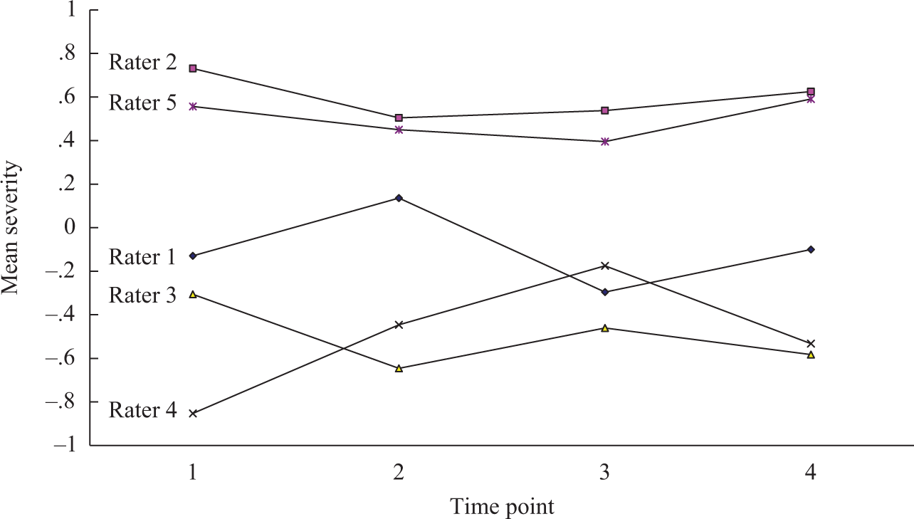
Mean severity for the five raters across time points.

Figure 3.

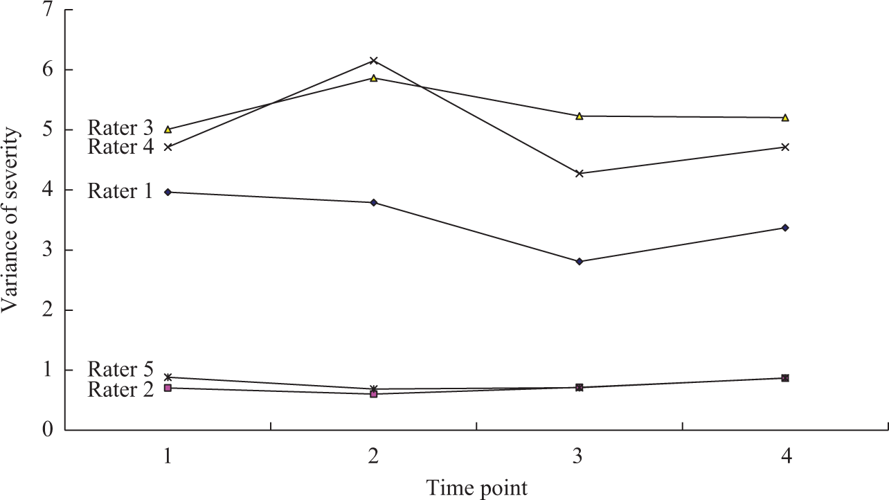
Variance of severity for the five raters across time points.

Conclusion

The generalized multilevel facets model for longitudinal data was developed. The model has three levels. At Level 1, a facets model is specified to describe item responses across time points. At Level 2, a latent trait growth model with an autoregressive residual structure that takes into account variation in the latent traits across measurement occasions within persons is formulated. In the latent trait growth model, a polynomial growth curve is specified to describe how the expected value of a response variable changes over time, and the covariance structure is autoregressive. At Level 3, a regression model is added to consider variation in growth trajectories between persons; it can be homoskedastic or heteroskedastic. The model parameters can be estimated with WinBUGS. The simulations show that WinBUGS yields fairly good parameter recovery, except for regression parameters at Level 2; the DIC and cross-validation log-likelihoods can be used for model comparison. In the empirical example, the data structure was a two-level one; a two-parameter model was more suitable than a one-parameter model; each item had its own step difficulties; each department had its own development trend; and Raters 2 and 5 were the strictest raters.

In this study, we applied a Bayesian hierarchical approach to the GMFM-L and used WinBUGS to analyze longitudinal data. The approach was proven to be efficient. While using a Bayesian approach, the specification of the prior distribution plays a crucial role (Gelman, 2006). This study uses a conjugate distribution, allowing WinBUGS to be used to estimate parameters easily. Multilevel prior specifications can be utilized to define hierarchical models.

The GMFM-L simultaneously considers an individual-based design data structure, missing data in persons and raters, and the interactions among persons, raters, and time points. As sample size is often small in longitudinal studies, the Bayesian hierarchical approach is able to provide more information on parameter estimation than that provided by the traditional non-Bayesian approach through prior information (Wollack, Bolt, Cohen, & Lee, 2002). With respect to repeated measurements, the GMFM-L allows autocorrelations and the Bayesian estimation method works directly on raw data and considers such dependence over time. The GMFM-L can easily deal with complex structures, such as factor analytic structures and multilevel structures. Furthermore, the GMFM-L divides errors into three parts to improve the reliability of analysis results.

Finally, analytical results show that a Bayesian approach can be applied directly in autoregressive residual models. However, because the samples are autocorrelated, WinBUGS converges very slowly. Improving convergence is very crucial for the GMFM-L. Future studies can investigate other programming languages (e.g., C or FORTRAN) or different sampling methods for achieving better convergence.

Footnotes

Appendix A: Second-Order Autoregressive Process

The second-order autoregressive process can be modeled as: (A.1)

ε_{t} = ϕ_{1} ε_{t - 1} + ϕ_{2} ε_{t - 2} + z_{t} .

Taking the variance of both sides of Equation (1) yields:

var (ε_{t}) = var (ϕ_{1} ε_{t - 1} + ϕ_{2} ε_{t - 2} + z_{t}) = var (ϕ_{1} ε_{t - 1}) + var (ϕ_{2} ε_{t - 2}) + var (z_{t}) + 2 ϕ_{1} ϕ_{2} cov (ε_{t - 1}, ε_{t - 2})

(A.2)

\begin{array}{l} = ϕ_{1}^{2} σ_{ε}^{2} + ϕ_{2}^{2} σ_{ε}^{2} + σ_{z}^{2} + 2 ϕ_{1} ϕ_{2} cov (ε_{t - 1}, ε_{t - 2}) \\ = (ϕ_{1}^{2} + ϕ_{2}^{2}) σ_{ε}^{2} + 2 ϕ_{1} ϕ_{2} γ_{1} + σ_{z}^{2} \equiv σ_{ε}^{2}, \end{array}

where

var (ε_{t - 1}) = var (ε_{t - 2}) = σ_{ε}^{2}, c o v (ε_{t - 1}, ε_{t - 2}) \equiv γ_{1}

. The process covariance γ₁ can be expressed in terms of model parameters ϕ₁, ϕ₂, and

σ_{ε}^{2}

as follows: (A.3)

cov (ε_{t - 1}, ε_{t - 2}) = E (ε_{t - 1} ε_{t - 2}) = E [(ϕ_{1} ε_{t - 2} + ϕ_{2} ε_{t - 3} + z_{t - 1}) ε_{t - 2}] = ϕ_{1} E (ε_{t - 2} ε_{t - 2}) + ϕ_{2} E (ε_{t - 3} ε_{t - 2})

(A.4)

= ϕ_{1} var (ε_{t - 2}) + ϕ_{2} γ_{1} = ϕ_{1} σ_{ε}^{2} + ϕ_{2} γ_{1} \equiv γ_{1 .} (i . e ., γ_{1} = ϕ_{1} σ_{ε}^{2} / (1 - ϕ_{2})) .

Equation (2) can be solved simultaneously with Equation (3) to obtain: (A.4)

σ_{ε}^{2} = \frac{(1 - ϕ_{2}) σ_{z}^{2}}{(1 + ϕ_{2}) (1 - ϕ_{2} + ϕ_{1}) (1 - ϕ_{2} - ϕ_{1})} .

If ϕ₂ = 0, then the AR(2) model reduces to the AR(1) model and

σ_{ε}^{2} = σ_{z}^{2} / (1 - ϕ_{1}^{2}) .

References

Adams

R. J.

Wilson

(1997). Multilevel item response models: An approach to errors in variables regression. Journal of Educational and Behavioral Statistics, 22, 47–76.

Albert

J. H.

Chib

(1993). Bayesian analysis of binary and polychotomous response data. Journal of the American Statistical Association, 88, 669–679.

Andersen

E. B.

(2004). Latent regression analysis based on the rating scale model. Psychology Science, 46, 209–226.

Andrich

(1978). A rating formulation for ordered response categories. Psychometrika, 43, 561–573.

Baker

F. B.

(1998). An investigation of the item parameter recovery characteristics of a Gibbs sampling approach. Applied Psychological Measurement, 22, 153–169.

Bartholomew

D. J.

(1981). Posterior analysis of the factor model. British Journal of Mathematical and Statistical Psychology, 34, 93–99.

Béguin

A. A.

Glas

C. A. W.

(2001). MCMC estimation of multidimensional IRT models. Psychometrika, 66, 541–561.

Christensen

K. B.

Bjorner

Kreiner

Petersen

J. H.

(2004). Latent regression in log linear Rasch models. Communications in Statistics, 33, 1295–1314.

Congdon

(2003). Applied Bayesian modeling. New York, NY: Wiley.

10.

Fox

J. P.

(2005). Multilevel IRT using dichotomous and polytomous items. British Journal of Mathematical and Statistical Psychology, 58, 145–172.

11.

Fox

J. P.

Glas

C. A. W.

(2001). Bayesian estimation of a multilevel IRT model using Gibbs sampling. Psychometrika, 66, 271–288.

12.

Geisser

Eddy

(1979). A predictive approach to model selection. Journal of the American Statistical Association, 74, 153–160.

13.

Gelfand

A. E.

(1996). Model determination using sampling-based methods. In Gilks

W. R.

Richardson

Spiegelhalter

D. J.

(Eds.), Markov Chain Monte Carlo in practice (pp. 145–161). London: Chapman-Hall.

14.

Gelman

(2006). Prior distributions for variance parameters in hierarchical models. Bayesian Analysis, 3, 515–534.

15.

Geman

(1984). Stochastic relaxation, Gibbs distribution and the Bayesian restoration of images. IEEE Transactions on Pattern Analysis an Machine Intelligence, PAMI-6, 721–741.

16.

Hastings

W. K.

(1970). Monte Carlo sampling methods using Markov chains and their applications. Biometrika, 57, 97–109.

17.

18.

Kamata

(2001). Item analysis by the hierarchical generalized linear model. Journal of Educational Measurement, 38, 79–93.

19.

Lee

(1981). A Bayesian approach to confirmatory factor analysis. Psychometrika, 46, 153–160.

20.

Linacre

J. M.

(1989). Many-facet Rasch measurement. Chicago, IL: MESA Press.

21.

Linacre

J. M.

(2002). Judging debacle in pairs figure skating. Rasch Measurement Transactions, 15, 839–840.

22.

Liu

J. S.

Sabatti

(2000). Generalized Gibbs sampler and multigrid Monte Carlo for Bayesian computation. Biometrika, 87, 353–369.

23.

Lunz

M. E.

Wright

B. D.

Linacre

J. M.

(1990). Measuring the impact of judge severity on examination scores. Applied Measurement in Education, 3, 331–345.

24.

Maier

K. S.

(2001). A Rasch hierarchical measurement model. Journal of Educational and Behavioral Statistics, 26, 307–330.

25.

Masters

G. N.

(1982). A Rasch model for partial credit scoring. Psychometrika, 47, 149–174.

26.

Metropolis

Rosenbluth

A. W.

Rosenbluth

M. N.

Teller

A. H.

Teller

(1953). Equation of state calculations by fast computing machines. The Journal of Chemical Physics, 21, 1087–1092.

27.

Mislevy

R. J.

(1985). Estimation of latent group effects. Journal of the American Statistical Association, 80, 993–997.

28.

Muraki

(1992). A generalized partial credit model: Application of an EM algorithm. Applied Psychological Measurement, 16, 159–176.

29.

Patz

R. J.

Junker

B. W.

(1999a). Applications and extensions of MCMC in IRT: Multiple item types, missing data, and rated responses. Journal of Educational and Behavioral Statistics, 24, 342–366.

30.

Patz

R. J.

Junker

B. W.

(1999b). A straightforward approach to Markov chain Monte Carlo methods for item response models. Journal of Educational and Behavioral Statistics, 24, 146–178.

31.

Raftery

A. E.

(1996). Approximate Bayes factor and accounting for model uncertainty in generalized linear models. Biometrika, 83, 251–266.

32.

33.

Roberts

G. O.

Smith

A. F. M.

(1993). Bayesian computation via the Gibbs sampler and related Markov chain Monte Carlo methods. Journal of the Royal Statistical Society, Series B, 55, 3–23.

34.

Scheines

Hoijtink

Boomsma

(1999). Bayesian estimation and testing of structural equation models. Psychometrika, 64, 37–52.

35.

Segawa

(2005). A growth model for multilevel ordinal data. Journal of Educational and Behavioral Statistics, 30, 369–396.

36.

Spiegelhalter

D. J.

Best

N. G.

Carlin

B. P.

Linde

A. V. D.

(2002). Bayesian measures of model complexity and fit. Journal of the Royal Statistical Society: Series B, 64, 583–639.

37.

38.

Tanner

M. A.

(1993). Tools for statistical inference: Observed data and data augmentation. 2nd ed.Berlin: Springer-Verlag.

39.

Tanner

M. A.

Wong

W. H.

(1987). The calculation of posterior distributions by data augmentation. Journal of the American Statistical Association, 82, 528–550.

40.

Wang

W. C.

Liu

C. Y.

(2007). Formulation and application of the generalized multilevel facets model. Educational and Psychological Measurement, 67, 583–605.

41.

Wang

W. -C.

Wilson

M. R.

(2005). Exploring local item dependence using a random-effects facet model. Applied Psychological Measurement, 29, 296–318.

42.

Wollack

J. A.

Bolt

D. M.

Cohen

A. S.

Lee

Y. S.

(2002). Recovery of item parameters in the nominal response model: A comparison of marginal maximum likelihood and Markov chain Monte Carlo estimation. Applied Psychological Measurement, 26, 337–350.

43.

Zhang

Hamagami

Wang

Grimm

K. J.

Nesselroade

J. R.

(2007). Bayesian analysis of longitudinal data using growth curve models. International Journal of Behavioral Development, 31, 374–383.

44.

Zhang

Nesselroade

J. R.

(2007). Bayesian estimation of categorical dynamic factor models. Multivariate Behavioral Research, 42, 729–756.

45.

Zwinderman

A. H.

(1991). A generalized Rasch model for manifest predictors. Psychometrika, 56, 589–600.