Identification of Average Treatment Effects in Social Experiments Under Alternative Forms of Attrition

Abstract

As any empirical method used for causal analysis, social experiments are prone to attrition which may flaw the validity of the results. This article considers the problem of partially missing outcomes in experiments. First, it systematically reveals under which forms of attrition—in terms of its relation to observable and/or unobservable factors—experiments do (not) yield causal parameters. Second, it shows how the various forms of attrition can be controlled for by different methods of inverse probability weighting (IPW) that are tailored to the specific missing data problem at hand. In particular, it discusses IPW methods that incorporate instrumental variables (IVs) when attrition is related to unobservables, which has been widely ignored in the experimental literature before.

Keywords

experiments attrition inverse probability weighting

1. Introduction

Causal inference based on experiments, which dates at least back to Neyman (1923) and Fisher (1925, 1935), is a cornerstone of the evaluation of policy interventions. It has been used in many different fields of research such as medicine, welfare policies, labor economics, education, and development economics; see for instance, the literature surveys in Duflo (2006), Harrison and List (2004), and Imbens and Wooldridge (2009). If well conducted and appropriate to the research question, experiments are widely regarded to be the most reliable source of causal inference; see for instance, Cochran and Chambers (1965), Freedman (2006), Rubin (2008), and Imbens (2009), as they invoke a minimum of identifying assumptions. They neither impose functional form assumptions as regression models nor particular correlations between observables and unobservables, which have to be assumed in observational studies. However, as any empirical method, experiments are prone to attrition which may flaw the validity of the results, see the discussion in Hausman and Wise (1979).

In this article, we consider the problem that the outcome of interest is only partially observed due to attrition, whereas the treatment and several socioeconomic characteristics, which are typically measured in baseline surveys prior to the intervention, are fully observed. Thus, attrition here refers to the censoring problem due to missing outcomes, but not to truncation, that is, the absence of information on the outcome, the treatment, and further variables for some subpopulation. The missing outcome problem arises, for instance, when individuals with known pretreatment characteristics are randomly assigned to an active labor market policy (such as a training), but some of them do not participate in a follow-up survey that measures labor market success (e.g., employment or income) several months or years later due to reluctance or relocation. Similar problems are inherent in clinical trials when some of the participants randomly assigned to medical treatments pass away before the health outcome is measured. Finally, suppose that high school students are randomly provided with private school vouchers and that we are interested in their scores obtained in college entrance examinations several years later. Attrition in the outcome arises if a subsample of students decides not to take the exam.

Various remedies have been proposed to deal with attrition in outcome data. Multiple imputation of missing values goes back to Rubin (1977, 1978); see also Rubin (1996) for a more recent review. Based on Bayesian techniques, the idea is to use multiple attrition models to impute multiple sets of plausible values for the missing data. This allows computing a probability interval for the parameter of interest. Several studies use single imputation methods such as regression adjustments to correct for attrition. For example, Hausman and Wise (1979) use a probability model of attrition in conjunction with a random effects model of individual response in their evaluation of the Gary Income Maintenance experiment. Angrist, Bettinger, and Kremer (2006) analyze the effects of school vouchers on test scores in college entrance examinations in Columbia and apply tobit regression to control for the fact that voucher winners are more likely to take the tests than voucher losers. Another approach is based on weighting observations according to their likelihood to respond, that is, by the inverse of their conditional response probability; see for instance, Scharfstein, Rotnitzky, and Robins (1999). The idea of inverse probability weighting (IPW) goes back to Horvitz and Thompson (1952), who first proposed an estimator of the population mean in the presence of nonrandomly missing data.

Barnard, Frangakis, Hill, and Rubin (2003) use a principal stratification framework (see Frangakis & Rubin, 2002) to estimate treatment effects under attrition (and further missing data and noncompliance problems) by means of a parametric mixture model. Still based on principal stratification, Mealli and Pacini (2008) exploit discrete instruments to identify effects for particular subgroups under various assumptions. Finally, the estimation of nonparametric bounds (see Horowitz & Manski, 1998, 2000) does not require a model for attrition at the cost of sacrificing point identification even for particular subpopulations. Empirical studies estimating bounds include Angrist et al. (2006), Lee (2009), and Grogger (2009), who assesses the effectiveness of Connecticut's Jobs First experiment. See also Zhang and Rubin (2003) and Zhang, Rubin, and Mealli (2008) who discuss the identification of bounds in a principal stratification framework.

This article makes two contributions to the literature on attrition in social experiments. First, it reveals systematically under which forms of attrition—in terms of its relation to observable or unobservable factors—experiments do (not) yield causal parameters, as a comprehensive discussion on attrition in experiments and its implications for identification is still lacking. Starting from a general treatment effect model, it makes explicit and formally discusses under which conditions experiments identify average treatment effects (ATEs) on the entire population and/or on the subpopulation of respondents.

Second, the article shows how the alternative forms of attrition can be controlled for by IPW methods, that is, by reweighting observations by the inverse of their conditional response and/or treatment probabilities. Depending on whether attrition is related to all or subsets of observable and unobservable variables, we will apply different weighting approaches, each of which is tailored to the specific attrition problem at hand. This provides practitioners with straightforward solutions depending on the suspected missing data problem. Simulation results presented further below suggest that assuming the wrong attrition process (e.g., by neglecting attrition related to unobservables) may do worse than not controlling for attrition at all. This underlines the importance of carefully thinking about the nature of attrition in order to choose an attrition model that is appropriate for the empirical application considered.

The use of IPW to control for attrition related to observables, that is, when outcomes are missing at random (MAR, see Rubin, 1976), is well established in the literature; see for instance, Robins and Rotnitzky (1995), Robins, Rotnitzky, and Zhao (1995), Rotnitzky and Robins (1995), Scharfstein et al. (1999), and Wooldridge (2002, 2007). In contrast, the case when attrition is related to unobservables such that identification requires an instrument for attrition (which does not directly affect the outcome variable) has been widely ignored in experiments. One of the very rare examples is DiNardo, McCrary, and Sanbonmatsu (2006) who use conventional sample selection correction techniques based on regression (see Heckman, 1976). The present work is the first that discusses the usefulness and application of IPW under attrition on unobservables in an experimental context. This approach is closely related to Huber (2009), who uses IPW to control for sample selection and attrition in observational studies.

Attrition related to unobservables is a problem likely to be found in many empirical problems. For example, suppose that motivation is not observed in a labor market policy or education experiment where the outcomes of interest are employment and earnings or test scores and educational achievement, respectively. While there is little doubt that motivation is correlated with these outcomes, there are also good reasons to believe that it affects the response behavior. For example, the least motivated individuals in a labor market policy experiment might be most reluctant to respond to the follow-up survey and unmotivated students are likely to be less inclined to participate in an exam than others. These and similar examples motivate the use of novel IPW methods based on continuous instruments for attrition. Unfortunately, such instruments, which are ideally randomly assigned in a similar way as the treatment, are rare in experiments conducted to date. Therefore, we argue that the creation of randomized instruments should be considered in the design of future experiments. Two potential instruments are the number of phone calls in follow-up surveys or financial incentives to respond to a survey.

Even though this study covers a range of attrition problems that are relevant in many empirical applications, the exposition is not exhaustive, as one can think of many different ways of modeling response behavior. For an alternative set of restrictions, see Imai (2009) who assumes that attrition is related to the outcome but is independent of the treatment conditional on the outcome and other observable variables. As the author argues, this is plausible when response behavior is strongly driven by the outcome variable (e.g., when considering the outcome “voting,” voters may be more willing to participate in postelection surveys than nonvoters), whereas the treatment represents only a mild intervention that is unlikely to affect attrition (e.g., a psychological voting stimulus). In contrast, we focus on scenarios where the treatment drives attrition even conditional on other variables (with the exception of the introductory case in which outcomes are missing completely at random [MCAR]). Whereas identification in Imai (2009) relies on controlling for the dependence between attrition and the treatment, we impose different assumptions that allow us to control for the dependence between attrition and the outcome.

The remainder of this article is organized as follows. The next section introduces a general treatment effect model along with attrition. Section 3 discusses identification under random attrition and attrition related to observables. Identification under attrition related to unobservables is treated in Section 4. Section 5 presents simulation studies based on both generated and empirical data. An application to a U.S. labor market policy experiment is provided in Section 6. Section 7 concludes.

2. Model

Let D denote a treatment indicator, either 1 (treatment) or 0 (nontreatment), which is randomly assigned to an independent and identically distributed (i.i.d.) sample of n units, indexed by $i = 1, \dots, n$ . We are interested in the effect of D on some outcome variable Y. Utilizing the potential outcome framework of Rubin (1974), we denote the potential outcome for individual i and some hypothetical treatment D = d as $Y_{i}^{d}$ , where $d \in {0, 1}$ . The difference $Y_{i}^{1} - Y_{i}^{0}$ would identify the individual treatment effect, but is unknown to the researcher, because each individual is either treated or not treated and cannot appear in both states of the world at the same time.

However, under particular assumptions a randomized experiment allows identifying treatment effects by the fact that the potential outcomes are independent of the treatment assignment. Throughout this article we will therefore rule out any interaction effects between the individuals participating in the experiment such as spill over, peer, or general equilibrium effects. This implies the validity of the Stable Unit Treatment Valuation Assumption (SUTVA); see, for instance, Rubin (1990). Furthermore, we will assume that treatment compliance is perfect, that is, everybody being assigned takes the treatment and everybody not assigned does not. If noncompliance occurred, identification would be further complicated. In this case, one might at best recover the effect on the subpopulation of the compliers (those behaving according to the assignment), given that the treatment assignment is a valid instrument for the realized treatment state. Even though we are fully aware that interaction effects and noncompliance in experiments (see, for instance, Robins & Tsiatis, 1991) may occur in practice, they are beyond the scope of this article. In the subsequent discussion, we will exclusively focus on the identification problems related to attrition in the outcome variable.

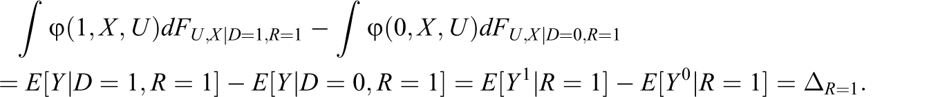
Under random treatment assignment, the expected potential outcomes are equal to the expected conditional outcomes given the treatment. Formally, $E [Y^{d}] = E [Y | D = d]$ for $d \in {0, 1}$ . Therefore, the ATE, denoted as $Δ$ , is identified by $E [Y | D = 1] - E [Y | D = 0]$ and is consistently estimated by the mean difference of treated and nontreated outcomes in the sample. Causal inference becomes less straightforward when the outcome variable is only partially observed due to attrition. The problems arising for identification and the remedies that may be used depend on how attrition is related to the treatment and the other parameters affecting the outcome.

To formally discuss the various forms of attrition, we consider a general treatment effect model. Assume that the outcome Y is an unknown function of the treatment, a vector of observed covariates X, and an unobserved term U.

Y = φ (D, X, U),

where

φ (\cdot)

is a general function. Throughout this article we will maintain the assumption that the treatment is randomly assigned:

Assumption 1:

D ⊥ (X, U),

that is, treatment D is independent of the joint distribution of X and U, where “

⊥

” denotes independence. When using the potential outcomes notation, this implies that

Y^{1}, Y^{0} ⊥ D

. In Section 3, we will also assume that X contains at least one continuously distributed variable. In Section 4, X may or may not be continuous.

This model provides us with a useful framework for the evaluation of policy interventions. Consider for instance the identification of the effect of vouchers for private schooling (D) to which high school students are randomly assigned on test scores in college entrance examinations (Y) several years later. Empirical evidence suggests that private schooling has an effect on test scores (see Angrist et al., 2006). Thus, we suspect the test scores to be a function of the treatment, but also of observed baseline characteristics (X) such as age and gender, which are usually provided in surveys accompanying randomized trials. Furthermore, also unobserved factors U such as motivation most likely influence the test scores. As a second example, consider labor market experiments where individuals are randomly assigned into a training; see, for instance, Bloom et al. (1997). The labor market outcomes (Y), for example, employment, unemployment, or income, are a function of training (D); socioeconomic characteristics like age, education, and gender (X); and unobservables (U) such as innate ability.

To introduce attrition into our framework, let R denote a binary response variable which is $1$ if Y is observed (nonattrition) and $0$ otherwise. In the context of the school voucher experiment, R represents test participation, as test scores are only observed conditional on taking part. In contrast, we will assume that (D, X) is observed for all individuals. The fact that only $Y | R = 1$ is known instead of $Y$ may flaw the validity of experimental results. The experiment bears external validity if it identifies the ATE on the entire population ( $Δ = E [Y^{1}] - E [Y^{0}]$ ) in spite of attrition. It bears internal validity if the ATE on the respondents, $Δ_{R = 1} = E [Y^{1} | R = 1] - E [Y^{0} | R = 1]$ , is identified. Whether external and/or internal validity holds depends on the nature of attrition. The following two sections will impose different assumptions on the relation between attrition and observed and unobserved factors in the treatment effect model and will discuss the implications for identification. When identification fails, we will propose IPW methods to correct for attrition bias and also discuss the required conditions.

While there is little doubt that Δ is an interesting policy parameter (even more so in experiments, where the ATE on the entire population is equal to the ATE on the treated population), the policy relevance of $Δ_{R = 1}$ is less clear as it only refers to the particular subpopulation of respondents. The latter might differ from the entire population in characteristics that are important for the effectiveness of the treatment such that Δ and $Δ_{R = 1}$ need not necessarily be similar. Therefore, we generally prefer to identify Δ rather than $Δ_{R = 1}$ if we have a choice. Indeed, with the exception of Newey (2007), the latter parameter has rarely been considered, neither in the sample selection literature, which usually assumes effect homogeneity across subpopulations (such that $Δ = Δ_{R = 1}$ ), nor in the standard treatment evaluation framework that abstracts from attrition.

However, under most forms of attrition, the identification of Δ requires somewhat stronger assumptions than the identification of $Δ_{R = 1}$ , which is intuitive because only $Y | R = 1$ is observed. If these stronger assumptions are not satisfied, identification among respondents appears to be the best we can get, see also the discussion in Newey (2007). In this case, it often seems preferable to identify at least $Δ_{R = 1}$ rather than not recovering any effect at all. Depending on the empirical context, this parameter may still bear policy relevance. For example, in the school voucher experiment it represents the ATE on the test takers that might be exactly what politicians want to learn about.

3. Identification Under Random Attrition and Attrition Related to Observables

The most innocuous form of attrition is the case when outcomes are MCAR; see, for instance, Rubin (1976) and Heitjan and Basu (1996). MCAR says that attrition is not related with any observed or unobserved parameter in the treatment effect model. After considering this benchmark case, we will systematically investigate more severe attrition problems.

Assumption 2:

R ⊥ (D, X, U) .

Assumption 2 states that attrition is independent of both observed and unobserved factors. Taking the school voucher experiment outlined in the last section as an example, it says that test participation is neither related to winning the school voucher nor to any other variables. This implies that the potential outcomes are independent of the response mechanism,

Y^{1}, Y^{0} ⊥ R

, and that the potential outcomes and the response mechanism are jointly independent of the treatment assignment,

(Y^{1}, Y^{0}, R) ⊥ D

. To see the implications for identification, note that the potential outcome under treatment

D = d

for individual i is

Y_{i}^{d} \equiv φ (d, X_{i}, U_{i})

for

d \in {0, 1}

. Furthermore, let

F_{A}

denote the cumulative distribution function (cdf) of a random variable A and

F_{A | B}

the conditional cdf given B. By MCAR,

\int φ (d, X, U) d F_{U, X | D = d, R = 1} = \int φ (d, X, U) d F_{U, X | D = d} = \int φ (d, X, U) d F_{U, X},

where the first equality follows from Assumption 2 and the second from Assumption 1. Therefore, the experiment bears external validity and identifies the ATE in spite of attrition:

\begin{aligned} \int φ (1, X, U) d F_{U, X | D = 1, R = 1} - \int φ (0, X, U) d F_{U, X | D = 0, R = 1} \\ = E [Y | D = 1, R = 1] - E [Y | D = 0, R = 1] = E [Y | D = 1] - E [Y | D = 0] \\ = E [Y^{1}] - E [Y^{0}] = Δ . \end{aligned}

As a first deviation from MCAR, we will now assume that response is a function of the treatment (e.g., winning a voucher for private schooling), but not of any other observed or unobserved parameter in the treatment effect model.

Assumption 3:

(3a) $R = I {ζ (D, V) \geq 0},$

(3b) $V ⊥ (X, U) .$

$I {\cdot}$ denotes the indicator function and $ζ (\cdot)$ denotes a general function. We assume V to be an unobserved term that is independent of (X, U) (3b). By (3a), D shifts R such that in general, $P r (D = 1 | R = 1)$ is different from $P r (D = 1)$ unless $ζ$ is of a very particular form. Note that a sufficient condition for $P r (D = 1 | R = 1) \neq P r (D = 1)$ is monotonicity of $ζ$ in its arguments. As D also affects Y, it follows that $E [Y | R = 1] \neq E [Y]$ because the share of treated individuals changes due to attrition. However, this does not affect identification, because the distribution of (X, U) is not related to the response behavior. This implies that $(Y^{1}, Y^{0}, R^{1}, R^{0}) ⊥ D$ , where $R^{d}$ denotes the hypothetical response for D = d, and $Y^{1}, Y^{0} ⊥ R | D$ . As under Assumption 2, it holds that

\int φ (d, X, U) d F_{U, X | D = d, R = 1} = \int φ (d, X, U) d F_{U, X | D = d} = \int φ (d, X, U) d F_{U, X} .

where the first equality follows from Assumption 3 and the second from Assumption 1. The experiment is again externally valid and identifies the ATE.

The forms of attrition considered under Assumptions 2 and 3 are unlikely to hold in many, if not most, social experiments. Empirical evidence suggests that response behavior is often related to the treatment and other observed characteristics; see, for instance, Hausman and Wise (1979), Fitzgerald, Gottschalk, and Moffitt (1998), and Grilo et al. (1998). These characteristics, X, are typically measured in baseline surveys prior to the intervention and commonly include gender, age, education, and other socioeconomic variables.

In the remainder of this section, we will assume that response is a function of the treatment and the covariates. In a first step, we impose a very particular relationship between X and D, namely, independence conditional on response. This case is primarily chosen for illustrative reasons rather than practical relevance. Interestingly, it entails internal validity of the experiment while external validity no longer holds without controlling for attrition.

Assumption 4:

(4a) $R = I {ζ (D, X, V) \geq 0},$

(4b) $V ⊥ (X, U),$

(4c) $X ⊥ D | R = 1.$

By Assumption 4, attrition affects the distributions of D and X, which are, however, not related to each other even conditional on response (4c). This implies that the distributional change in X is equal across treatment states. For example, assume that X represents age in our school voucher experiment and that it is positively related with response (i.e., older students are more likely to take the test). Then, the age composition must change in the same manner for voucher winners and losers when conditioning on test participation. As U does not affect the response, the joint distribution of (X, U) conditional on R = 1 is independent of D. Thus, $\int φ (d, X, U) d F_{X, U | D = d, R = 1} = \int φ (d, X, U) d F_{X, U | R = 1}$ . The mean potential outcome of respondents is equal to the average conditional outcome given D = d among respondents. Therefore, the experiment identifies the ATE on respondents ( $Δ_{R = 1}$ ) and is internally valid:

\begin{aligned} \int φ (1, X, U) d F_{U, X | D = 1, R = 1} - \int φ (0, X, U) d F_{U, X | D = 0, R = 1} \\ = E [Y | D = 1, R = 1] - E [Y | D = 0, R = 1] = E [Y^{1} | R = 1] - E [Y^{0} | R = 1] = Δ_{R = 1} . \end{aligned}

However, it is not externally valid, which would require that $Δ_{R = 1} = Δ$ . The latter does not hold because the distribution of X is not the same for respondents and nonrespondents such that $\int φ (d, X, U) d F_{X, U | R = 1} \neq \int φ (d, X, U) d F_{X, U}$ .

Under certain conditions, the ATE on the entire population is identified by weighting respondents according to the likelihood that their observed characteristics appear in the entire population. To this end, we define the response propensity score (see Rosenbaum & Rubin, 1983), that is, the conditional response probability given (D, X), as $p (D, X) \equiv P r (R = 1 | D, X)$ . Furthermore, we impose the following common support restriction:

Assumption 4’:

P r (R = 1 | D = d, X = x) > c f o r a l l x \in χ, d \in {0, 1}, c > 0.

χ denotes the support of X. Assumption 4’ states that for any (D, X), the response probability must be bounded away from zero, otherwise outcomes are never observed for particular combinations of the treatment and the covariates. This allows us to reestablish external validity of the experiment by IPW as suggested in Proposition 1.

Proposition 1:

Under Assumptions 1, 4, and 4’, the ATE is identified by

Δ = E [\frac{R \cdot Y}{p (1, X)} | D = 1] - E [\frac{R \cdot Y}{p (0, X)} | D = 0] .

Proof: See Appendix A, available online at http://jeb.sagepub.com/supplemental.

Thus, weighting observations by the inverse of their respective response propensity score identifies the ATE. The idea of using IPW to control for attrition or similar selection problems goes back to Horvitz and Thompson (1952), who proposed an estimator of the population mean when data are missing nonrandomly. IPW has been frequently applied when the attrition process is assumed to depend only on observables, that is, when outcomes are MAR in the notation of Rubin (1976). Formally, the MAR requires that

P r (R = 1 | D, X, Y) = 1.5 p t P r (R = 1 | D, X)

, or equivalently, that

Y ⊥ R | D, X

. For example, Robins and Rotnitzky (1995), Robins et al. (1995), Rotnitzky and Robins (1995), and Scharfstein et al. (1999) use IPW to adjust for missing data in regression models. Wooldridge (2002) considers IPW M-estimation of missing data models, and Proposition 1 fits into his general framework as a special case.

To make our framework more general, we relax Assumption 4 somewhat by omitting Assumption (4c). This allows the gradient of X on the response process to differ across treatment states. For example, one could imagine that in the school voucher experiment, private schools (D = 1) are equally successful in sending younger and older students ( $X$ = age) to college entrance examinations (R = 1), whereas public schools (D = 0) more likely send older students. This would change the distribution of X across treatments among test takers.

Assumption 5:

(5a) $R = I {ζ (D, X, V) \geq 0},$

(5b) $V ⊥ (X, U) .$

Without further assumptions, $\int φ (d, X, U) d F_{X, U | D = d, R = 1} \neq \int φ (d, X, U) d F_{X, U | R = 1}$ . Thus, internal validity no longer holds because the distribution of X generally differs across treatment states among respondents such that the effect of D is confounded. However, it still holds that

\begin{aligned} \int φ (d, X, U) d F_{U | D = d, X = x, R = 1} = \int φ (d, X, U) d F_{U | D = d, X = x} \\ = \int φ (d, X, U) d F_{U | X = x} f o r a l l x \in χ, \end{aligned}

where the first equality follows from the randomness of response conditional on (D, X) implied by Assumption 5, which satisfies MAR, and the second from Assumption 1. Note that this would also hold if we relaxed (5b) somewhat to

V ⊥ U | X

It follows that the mean potential outcome among respondents is

\int \int φ (d, X, U) d F_{U | D = d, X = x, R = 1} d F_{X | R = 1} .

This allows us to identify the ATE on the respondents and to reestablish internal validity. Similarly to the response propensity score, we define the treatment propensity score among respondents, that is, the conditional treatment probability given X, as

π (X) \equiv P r (D = 1 | X, R = 1)

and impose the following common support assumption:

Assumption 5’:

Δ_{R = 1} = E [\frac{D \cdot Y}{π (X)} - \frac{(1 - D) \cdot Y}{1 - π (X)} | R = 1] .

Assumption 5’ states that the treatment propensity score is bounded away from 0 and 1, which rules out arbitrarily large weights in the subsequent proposition that reestablishes internal validity of the experiment.

Proposition 2:

Under Assumptions 1, 5, and 5’, the ATE on respondents is identified by

Δ_{R = 1} = E [\frac{D \cdot Y}{π (X)} - \frac{(1 - D) \cdot Y}{1 - π (X)} | R = 1] .

Proof: See Appendix B, available online at http://jeb.sagepub.com/supplemental

By reweighting the outcomes of respondents by the inverse of the (non)treatment propensity score, we control for differences in the distributions of X across treatment states conditional on response to identify

Δ_{R = 1}

. This is analogous to the application of IPW in a “selection on observables” or “conditional independence” framework; see, for instance, Hirano, Imbens, and Ridder (2003). The difference is that in the latter case, the imbalances in X exist even without attrition due to nonrandom assignment, whereas here, they only occur conditional on response. Yet, similar remedies can be applied to both problems, but note that Hirano et al. (2003) identify Δ (not

Δ_{R = 1}

However, under somewhat stronger common support conditions, we can even identify the ATE on the entire population and reestablish external validity. To this end, note that the mean potential in the entire population is

\int \int φ (d, X, U) d F_{U | D = d, X = x, R = 1} d F_{X} .

That is, integrating over the distribution of X in the entire population identifies the potential outcomes and the ATE. As for Proposition 1, this requires that the response probability is bounded away from zero for any (D, X).

Proposition 3:

Under Assumptions 1, 4’, 5, and 5’, the ATE is identified by

Δ = E [\frac{R \cdot D \cdot Y}{p (D, X) \cdot π (X)} - \frac{R \cdot (1 - D) \cdot Y}{p (D, X) \cdot (1 - π (X))}] .

Proof: See Appendix C, available online at http://jeb.sagepub.com/supplemental.

Δ is identified by using

π (X)

to adjust for differences in the distributions of X across D among respondents and p(D, X) to control for differences in (D, X) between respondents and nonrespondents. Note that the strong Assumption (5b) may be replaced by the less severe restriction

V ⊥ U | D, X

, which might be considerably more plausible in empirical applications. Even then, response is random conditional on (D, X), MAR is satisfied, and Propositions 2 and 3 still apply.

4. Identification Under Attrition Related to Unobservables

In the last section we considered various forms of attrition related to observables. In our treatment effect model, MAR requires that U and V, the unobserved terms in the outcome and response equations, are independent, at least conditional on observed characteristics. This assumption will be no longer maintained in this section. Instead, we will assume attrition on unobservables by allowing for a nonzero correlation between U and V even conditional on D, X. Analogous to sample selection models (see Heckman 1974, 1976, 1979)—at least when identification is nonparametric (e.g., Das, Newey, & Vella, 2003; Huber, 2009; Newey, 2007)—point identification hinges on the availability of an instrument that affects response but has no direct effect on the outcome.

Reconsider the school voucher experiment in which only a subpopulation takes the test. Assume that the probability to take the test is a function of unobserved motivation and ability which are correlated with tests scores even conditional on the treatment and observed characteristics (e.g., age and gender). Then, identification requires an instrument that shifts test participation but has no direct effect on the test scores.

Assumption 6:

(6a) $R = I {ζ (D, X, Z) \geq V},$

(6b) Cov $(U, V) \neq 0$ (and Cov $(U, V) \neq 0 | D, X)$ .

By Assumption 6, R is a function of at least one element that is excluded in $φ$ , namely, the instrument Z. Due to the nonzero covariance of V and U, the effect of D on Y among respondents is confounded even conditional on X. Identification requires Z to be a good predictor for R, to contain at least one continuous element, and not to have a direct effect on the outcome. The following restrictions guarantee the validity of the instrument.

Assumption 6’:

(6’a) Cov $(Z, R | D, X) \neq 0$ and $Y ⊥ Z | D, X$ ,

(6’b) $P r (R = 1 | D = d) > c$ , $c > 0$ , $d \in {1, 0}$ ,

(6’c) $(U, V) ⊥ (D, Z)$ ,

(6’d) $F_{V} (t)$ , the cdf of V, is strictly monotonic in the argument $t$ .

Assumption (6’a) states that Z shifts R but is not directly related with Y. Assumption (6’b) rules out that being treated or nontreated predicts attrition perfectly. For example, not winning a school voucher must not rule out test participation. To see the usefulness of this assumption, assume the opposite such that units with D = 0 never respond independent of the values of (X, Z). Obviously, the treatment effect cannot be evaluated as no comparisons with D = 0 are available in the subpopulation of respondents.

By (6’c), we impose that (D, Z) are jointly independent of the unobservables (U, V). Independence between (U, V) and D is satisfied by the randomization of the treatment if V is not a posttreatment variable. Still, it needs to be plausibly argued that $(U, V) ⊥ Z$ . In the school voucher experiment, where we only observe test scores conditional on test participation, one might think of distance or transportation costs to the test center as a valid instrument if it is plausibly unrelated to unobserved motivation and ability. However, there may exist credible concerns that the distribution of motivation differs for students close and distant to the test center such that Assumption (6’c) is violated. For example, if families with higher educated parents systematically choose neighborhoods closer to the test centers for some reason (e.g., central location or good infrastructure) and if higher educated parents also better motivate their children to strive for a higher education, then the instrument is not independent of the unobserved terms.

As argued by DiNardo et al. (2006), the instrument should ideally be randomly assigned in a similar way as the treatment. This would plausibly justify Assumption (6’c). For example, in a follow-up telephone survey, Z may be the number of phone calls per experimental unit which is randomized prior to the treatment assignment. A higher number of attempted calls should increase the response probability while being unrelated with other factors under random assignment. Also financial incentives are likely to affect response behavior (see Castiglioni, Pforr, and Krieger, 2008). In the school voucher example, students could be randomly offered different levels of cash payments or refunding of travel expenses in the case that they take the test. Of course, one would need to unambiguously communicate that the payment is conditional on participation alone, not on the test score (otherwise the motivation to prepare oneself for the test is likely to be affected). A further example would be the randomization of the distance to the test center, given that the choice of various test locations is feasible in the experimental design. Note that (6’c) could be relaxed to $(U, V) ⊥ (D, Z) | X$ , that is, conditional independence given observed variables (such as parents' education), which might be more plausible in applications without randomized instruments.

Concerning Assumption (6’d), first note that $P r (R = 1 | D, X, Z) = P r (ζ (D, X, Z) \geq V) = F_{V} (ζ (D, X, Z))$ . Assumption (6’d) states that the likelihood to respond increases strictly monotonically in $ζ$ . This allows us to back out the distribution of V by pinning down (D, X, Z). By comparing individuals with the same response propensity score we control for V and, thus, also for the dependence between V and U. Without strict monotonicity, a 1:1 relation between $F_{V} (t)$ and $ζ$ would not exist such that $P r (R = 1 | D, X, Z)$ would generally not correspond to a unique value of V. Under (6’d), however, V can be fixed to rule out confounding of the treatment effect due to attrition related to unobservables. That is, the response propensity score serves as a control function where the exogenous variation comes from Z. Control functions have been applied in semi- and nonparametric sample selection models, for example, Ahn and Powell (1993) and Das, Newey, and Vella (2003), as well as in nonparametric models with endogeneity; see, for example, Newey, Powell, and Vella (1999), Blundell and Powell (2003), and Imbens and Newey (2009). Furthermore, strict monotonicity is implicit in linear index restrictions used in the parametric sample selection literature (see Heckman, 1974, 1976, 1979).

However, conditioning on the response propensity score alone does not suffice for causal inference. A first reason is that, similar to Assumptions 4 and 5, response is a function of X and D. Therefore, random treatment assignment does not necessarily entail independence of D and X among respondents, as the distribution of X might differ across treatment states conditional on R = 1. Second, this is even more likely to be the case conditional on the response propensity score. To see this, note that individuals in different treatment states D but with equal values of X and Z must have distinct response propensity scores. That is, $P r (R = 1 | D = 1, X = x, Z = z) \neq P r (R = 1 | D = 0, X = x, Z = z)$ . As we need to compare treated and nontreated individuals with identical response propensity scores to control for the attrition bias, these individuals necessarily differ with respect to (X, Z). Despite the randomization of the treatment in the entire population, identification requires conditioning on both the response propensity score and the covariates among respondents. That is, conditional on X = x we need to compare the outcomes of treated and nontreated observations that satisfy $P r (R = 1 | D = 1, X = x, Z = z^{'}) = P r (R = 1 | D = 0, X = x, Z = z^{''})$ for some $z^{'}, z^{''}$ in the support of Z. This generally forces the instrument to include at least one continuous element, otherwise comparable treated and nontreated observations might not exist.

We will now formally discuss identification. For notational ease, let $W \equiv (D, X, Z)$ and the response propensity score $p (W) \equiv P r (R = 1 | D, X, Z)$ . Under Assumption (6’c), U and D are independent conditional on p(W) and X, which can be shown analogously to the proof of Theorem 1 in Newey (2007). Let a(U) denote any bounded function of U. Note that ${R = 1} = {F_{V}^{- 1} (p (W)) \geq V}$ . Then,

\begin{array}{c} E [a (U) | D, X, p (W), R = 1] = E [E [a (U) | V, D, X, Z] | D, X, p (W), F_{V}^{- 1} (p (W)) \geq v] \\ = E [E [a (U) | V, X] | D, X, p (W), F_{V}^{- 1} (p (W)) \geq v] \\ 0.5 p c = E [E [a (U) | V, X] | X, p (W), F_{V}^{- 1} (p (W)) \geq v] \\ = E [E [a (U) | V, X, p (W)] | X, p (W), R = 1] \\ - 3 p c = E [a (U) | X, p (W), R = 1], \end{array}

where the first equality follows from iterated expectations, the second and third from (6’c), the fourth from the fact that

E [E [A | B] | B, C] = E [E [A | B, C] | B, C]

for any variables A, B, and C, and the last from a backward application of the law of iterated expectations.

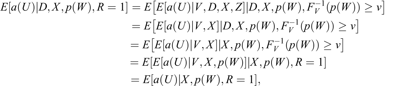
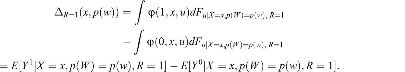
Thus, treatment effects are identified by conditioning on the response propensity score and the covariates. To see this, note that the conditional ATE given X and p(W) conditional on response is defined as

\begin{array}{c} Δ_{R = 1} (x, p (w)) = \int φ (1, x, u) d F_{u | X = x, p (W) = p (w), R = 1} \\ - \int φ (0, x, u) d F_{u | X = x, p (W) = p (w), R = 1} \\ = E [Y^{1} | X = x, p (W) = p (w), R = 1] - E [Y^{0} | X = x, p (W) = p (w), R = 1] . \end{array}

E [Y^{d} | X = x, p (W) = p (w), R = 1]

is the expected potential outcome for a hypothetical treatment d given X and p(W) among respondents. By the conditional independence of U and D given p(W) and X, it holds that

\begin{aligned} E [Y^{d} | X = x, p (W) = p (w), R = 1] = \int φ (d, x, u) d F_{u | X = x, p (W) = p (w), R = 1} \\ = \int φ (d, x, u) d F_{u | D = d, X = x, p (W) = p (w), R = 1} \\ = E [Y | D = d, X = x, p (W) = p (w), R = 1] . \end{aligned}

Hence, the expected potential outcome is equal to the expected conditional outcome, given D = d. The ATE on respondents

Δ_{R = 1}

is identified by the integration over the marginal distributions of X and p(W) in the subpopulation with observed outcomes.

\begin{aligned} \int \int [E [Y | D = 1, X = x, p (W) = p (w), R = 1] \\ - E [Y | D = 0, X = x, p (W) = p (w), R = 1]] d F_{x | p (W) = p (w), R = 1} d F_{p (w) | R = 1} \\ = \int \int [E [Y^{1} | X = x, p (W) = p (w), R = 1] \\ - E [Y^{0} | X = x, p (W) = p (w), R = 1]] d F_{x | p (W) = p (w), R = 1} d F_{p (w) | R = 1} \\ = E [Y^{1} - Y^{0} | R = 1] = Δ_{R = 1} . \end{aligned}

Therefore, the identification of

Δ_{R = 1}

hinges on the common support of the treatment in X and

p (W)

. Δ is not identified without further assumptions (see also Newey, 2007), as Y is not even observed when R = 0. However, under the additional restrictions that the response propensity score is positive for any (X, p(W)) and that Y is homoscedastic conditional on (D, X) one also identifies the ATE on the entire population. To this end, we impose the following assumption:

Assumption 6”:

(6”a) $\scale 95$ for all $x$ $\in$ χ, for all $Z$ $\in$ $Z$ ,

(6”b) $c < P r (D = 1 | X = x, p (W) = p (w)) < 1 - c$ , for all $x$ $\in$ χ, for all $5 p t p (w)$ $\in$ $P$ , $c > 0$ ,

(6”c) $Y = φ (D, X) + U$ .

$Z$ and $P$ denote the support regions of Z and p(W). Note that (6”a) is stronger than (6’b). Effects on the entire population could not be identified if there existed individuals with a response propensity score equal to zero, as this would rule out suitable comparisons in the subpopulation of respondents. Assumption (6”c) decreases the generality of our model due to separability of the observed and unobserved terms (see also Das et al., 2003), but ensures homoscedasticity of Y given (D, X). This is required for the identification of Δ, as outlined further below. Similar to the last section, let $π (X, p (W))$ denote the treatment propensity score, $π (X, p (W)) \equiv P r (D = 1 | X, p (W), R = 1)$ . Propositions 4 and 5 show identification of the ATEs on the respondents and on the entire population.

Proposition 4:

Under Assumptions 1, 6, 6’, and (6”b), the ATE on the respondents is identified by

Δ_{R = 1} = E [\frac{D \cdot Y}{π (X, p (W))} | R = 1] - E [\frac{(1 - D) \cdot Y}{1 - π (X, p (W))} | R = 1] .

Proof: See Appendix D, available online at http://jeb.sagepub.com/supplemental.

By weighting observations by the inverse of the (non-)treatment propensity score, we adjust for differences in the distributions of X and p(W) between treated and nontreated respondents. Proposition 4 is similar to Proposition 3, with the exception that we have to additionally condition on the response propensity score in the treatment propensity score to control for attrition on unobservables.

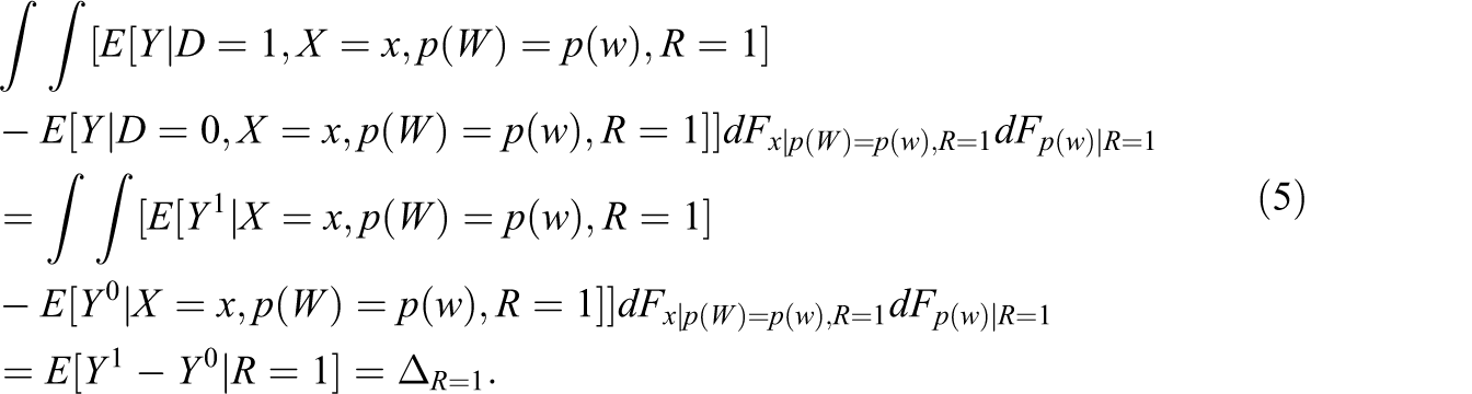
It seems useful to compare our approach based on the propensity score and a continuous instrument to Mealli and Pacini (2008) who control for attrition by conditioning on a binary instrument ( $Z$ $\in$ {0,1}) directly. This allows them to classify the population into subgroups (or “latent strata”) according to their response behavior conditional on hypothetical values of the treatment and the instrument (here for a given X). Identification relies (among other restrictions) on the fact that attrition is random for individuals with the same response behavior. One assumption considered by Mealli and Pacini (2008) is a perfect instrument: R = 1 always holds if Z = 1, such that treated and nontreated individuals with Z = 1 have the same response behavior. In terms of the response propensity score, this implies that $p (D = 1, X = x, Z = 1) = p (D = 0, X = x, Z = 1) = 1$ .

This example illustrates that conditioning on the propensity score is equivalent to conditioning on the response behavior, which can be easily shown in a principal stratification framework. For this reason and as already discussed before, effects are identified if particular combinations of D and Z yield the same response propensity scores across treatment states (which need not necessarily be equal to one) for a given X, for example, if $p (D = 1, X = x, Z = 0) = p (D = 0, X = x, Z = 1)$ . However, for a discrete Z, the existence of comparable propensity scores across treatment states does not hold in general (not even for a subpopulation) such that Mealli and Pacini (2008) also consider further assumptions. In contrast, it holds in the presence of a sufficiently strong continuous instrument. There obviously exists a trade-off between identification and econometric feasibility between the two approaches if the instrument is not perfect. Discrete instruments, on one hand, are easier to find in empirical applications but only allow for partial identification or at best point identification in some subpopulation. Continuous instruments, on the other hand, are very hard to find in reality, but have more identifying power. They even allow us to identify the ATE on the entire population, given that the common support Assumption 6” is satisfied.

Proposition 5:

Under Assumptions 1, 6, 6’, and 6”, the ATE is identified by

Δ = E [\frac{R \cdot D \cdot Y}{p (W) \cdot π (X, p (W))}] - E [\frac{R \cdot (1 - D) \cdot Y}{p (W) \cdot (1 - π (X, p (W)))}] .

Proof: See Appendix E, available online at http://jeb.sagepub.com/supplemental.

The ATE on the entire population is identified based on reweighting observations (in addition to the inverse treatment propensity score) by the inverse of the response propensity score, that is, by using the relative likelihood of a particular triple (D, X, Z) to appear in the entire population, as weighting function.

This result may seem surprising, given the fact that outcomes are only partially observed and observed outcomes do not allow inferring on the unobserved outcomes. That is, $E [Y | D = d, X = x, p (W) = p (w), R = 1] \neq E [Y | D = d, X = x, p (W) = p (w), R = 0]$ due to different conditional distributions of the unobserved term U. Nevertheless, Assumptions 6’ and 6” imply that $Δ_{R = 1} (x, p (w)) = Δ_{R = 0} (x, p (w))$ . To see this, note that $F_{U | D = d, X = x, p (W) = p (w), R = r} = F_{U | X = x, p (W) = p (w), R = r}$ for $r \in {0, 1}$ by (6’c) such that

\begin{array}{c} Δ_{R = 1} (x, p (w)) = \int [φ (1, x) + u] d F_{U | X = x, p (W) = p (w), R = 1} \\ - \int [φ (0, x) + u] d F_{U | X = x, p (W) = p (w), R = 1}, \\ Δ_{R = 0} (x, p (w)) = \int [φ (1, x) + u] d F_{U | X = x, p (W) = p (w), R = 0} \\ - \int [φ (0, x) + u] d F_{U | X = x, p (W) = p (w), R = 0} . \end{array}

Δ_{R = 1} (x, p (w))

and

Δ_{R = 0} (x, p (w))

only differ with respect to the integrals over different conditional distributions of U, given R = 1 and R = 0, which cancel out in the subtractions by (6”c). Thus,

Δ_{R = 1} (x, p (w)) = Δ_{R = 0} (x, p (w))

. Therefore, reweighting the conditional treatment effects of the respondents according to the distribution of (D, X, Z) in the entire population identifies Δ.

For completeness, we will briefly discuss identification under a particular deviation from the previous model, assuming that response is a function of D, Z, and V, but is not related with the covariates X.

Assumption 7:

(7a) $R = I {ζ (D, Z) \geq V},$

(7b) Cov $(U, V) \neq 0$ .

Under this particular form of attrition, the response behavior is merely a function of the treatment and unobservables but unrelated to the observed covariates. Whether Assumption 7 is plausible depends on the evaluation problem at hand and may even be tested (by testing the explanatory power of X on R). The response propensity score is now $p (D, Z) \equiv P r (R = 1 | D, Z)$ . We impose the following instrumental variable (IV) and common support assumptions.

Assumption 7’:

(7’a) Cov $(Z, R | D) \neq 0$ and $Y ⊥ Z | D$ ,

(7’b) $P r (R = 1 | D = d) > c$ , $c > 0$ , $d \in {1, 0}$ ,

(7’c) $(X, U, V) ⊥ (D, Z)$ ,

(7’d) $F_{V} (t)$ , the cdf of V, is strictly monotonic in the argument $t$ .

Assumption 7”:

(7”a) $P r (R = 1 | D = d, Z = z) > c, c > 0,$ for all $x$ $\in$ χ, for all $Z$ $\in$ $Z$ ,

(7”b) $c < P r (D = 1 | p (D, Z) = p (d, z)) < 1 - c$ , for all $x$ $\in$ χ, for all $p (d, z)$ $3 p t \in$ $P$ , $c > 0$ ,

(7”c) $Y = φ (D, X) + U$ .

Assumptions 7’ and 7” are straightforward modifications of 7’ and 7”, with the exception of (7’c), which assumes independence of the (D, Z) also with respect to X. Again, the treatment is independent by randomization, whereas the independence of Z and X may or may not be plausible and might be tested. By Assumptions 1, 7, and (7’c) it holds that X is independent of D conditional on p(D, Z) and R = 1, because $F_{X | D, p (D, Z), R = 1} = F_{X | D} = F_{X}$ . Therefore, treatment effects are identified conditional on p(D, Z) or on the simplified treatment propensity score $π (p (D, Z)) \equiv P r (D = 1 | p (D, Z))$ , respectively. Similar to Propositions 4 and 5, the ATEs on the respondents and the entire population can be expressed by the following equations:

Proposition 6:

Under Assumptions 1, 7, 7’, and (7”b), the ATE on the respondents is identified by

Δ_{R = 1} = E [\frac{D \cdot Y}{π (p (D, Z))} | R = 1] - E [\frac{(1 - D) \cdot Y}{1 - π (p (D, Z))} | R = 1] .

Proof: See Appendix F, available online at http://jeb.sagepub.com/supplemental.

Proposition 7:

Under Assumptions 1, 7, 7’, and 7”, the ATE is identified by

Δ = E [\frac{R \cdot D \cdot Y}{p (D, Z) \cdot π (p (D, Z))}] - E [\frac{R \cdot (1 - D) \cdot Y}{p (D, Z) \cdot (1 - π (p (D, Z)))}] .

Proof: See Appendix G, available online at http://jeb.sagepub.com/supplemental.

In the last two sections, we have covered several forms of attrition and provided a guideline on which weighting methods are appropriate under specific assumptions. In particular, the use of IPW incorporating IVs when attrition is on unobservables has been discussed, a case widely ignored in the experimental literature. The subsequent sections will present simulation results and an empirical application to a U.S. labor market policy experiment.

5. Simulation Studies

In this section, we run a horse race between the experimental mean difference estimator not controlling for attrition and IPW estimators assuming that attrition is related to observables and unobservables as treated under Assumptions 5 and 6, respectively. For this reason, we conduct simulation studies based on both generated and empirical data. Starting with the former scenario, we consider the following data generating process (DGP):

\begin{aligned} Y_{i} = α_{1} D_{i} + α_{2} X_{i} + α_{2} D_{i} X_{i} + U_{i}, \\ Y_{i} i s o b s e r v e d i f R_{i} = 1, \\ R_{i} = I {β_{1} D_{i} + β_{2} X_{i} + β_{3} Z_{i} + V_{i} > 0} . \end{aligned}

Apart from the treatment D, the covariate X, and the unobserved term U, the outcome Y also depends on an interaction term of D and X, which introduces effect heterogeneity with respect to X. X and Z are uniformly distributed with support regions [–1, 1] and [–1, 2], respectively. D is Bernoulli and either 1 or 0 with equal probability. (U, V) are drawn from a multivariate standard normal distribution. Their covariance is set to zero in the case of attrition on observables and to

0.8

under attrition on unobservables. The coefficients in the outcome equation are set to

α_{1} = α_{2} = 1, α_{3} = .25

. Under attrition on observables

β_{1} = β_{2} = 1

and

β_{3} = 0

such that roughly two thirds of the outcomes are observed. Under attrition on unobservables,

β_{1} = β_{2} = 0.5

and

β_{3} = 1

, that is,

R

is also a function of the instrument

Z

, which is excluded from the outcome equation. Approximately 70% of the outcomes are observed in this case.

We use normalized versions (such that weights add up to unity, see Imbens, 2004; Busso, DiNardo, & McCrary, 2009b) of the sample analogs of Propositions 2, 3, 4, and 5 as estimators of the ATE on the entire population (denoted as $\hat{Δ}$ ) and on the respondents ( ${\hat{Δ}}_{R = 1}$ ). The response and treatment propensity scores $p (W), π (X, p (W))$ are specified as probit models. We run 2,000 Monte Carlo simulations for two different sample sizes (n = 500, 2,000) and compare the accuracy of IPW estimators to naively taking mean differences of treated and nontreated outcomes among respondents. The following tables report the results for untrimmed IPW estimators as hardly any propensity score estimate in any Monte Carlo replication is close to the boundaries of 0 and 1. Therefore, methods incorporating propensity score trimming (see, for instance, Busso, DiNardo, & McCrary, 2009a; Crump, Hotz, Imbens, & Mitnik, 2009) yield virtually the same results and are omitted in the article, but are available upon request.

Table 1 displays the estimates, bias, standard errors (SE) and mean squared errors (MSEs) for the different methods when attrition is related to observables. Note that the ATEs on the entire population and on the respondents are normalized to unity. The IPW estimators following from Propositions 2 and 3 are effective in controlling for attrition bias. $\hat{Δ}, {\hat{Δ}}_{R = 1}$ are close to the true values and their accuracy in terms of MSE increases in the sample size. In contrast, the mean difference estimator is substantially biased. For the estimation of the ATE on the entire population under the smaller sample size it is, however, competitive in terms of the MSE. This is due to its smaller variance compared to IPW, which introduces additional uncertainty through the estimation of two propensity scores. Under the larger sample size, the persistence of the bias of the mean difference estimator dominates its better precision, such that IPW is clearly superior. In conclusion, the simulation results suggest that IPW is likely to reduce the MSE if the sample size is sufficiently large. Note that many recently conducted social experiments exceed the sample sizes considered in the simulations and typically contain several thousand observations, for example, Angrist et al. (2006), Angrist and Lavy (2009), Bertrand and Mullainathan (2004), Gertler (2004), and Krueger and Zhu (2004), or even more (Karlan & List, 2007).

Table 1.

Attrition on Observables, Simulated Data

	$\hat{Δ}$	Bias	SE	MSE	${\hat{Δ}}_{R = 1}$	Bias	SE	MSE
n = 500
IPW obs mean difference true effect (normalized)	1.001	0.001	0.180	0.032	0.998	−0.002	0.112	0.012
	0.883	−0.117	0.135	0.032	0.851	−0.149	0.130	0.039
	1.000				1.000
$n$ = 2,000
IPW obs mean difference true effect (normalized)	1.000	0.000	0.087	0.008	0.998	−0.002	0.056	0.003
	0.882	−0.118	0.066	0.018	0.849	−0.151	0.064	0.027
	1.000				1.000

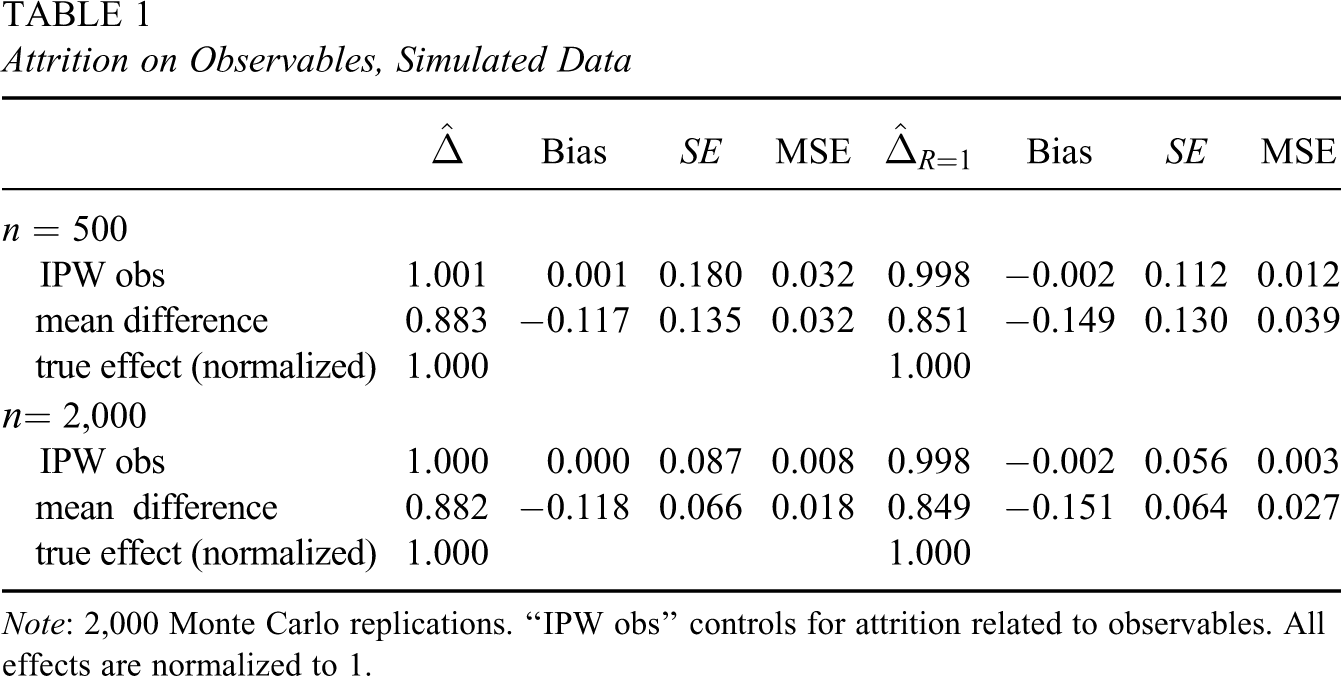
Note: 2,000 Monte Carlo replications. “IPW obs” controls for attrition related to observables. All effects are normalized to 1.

Table 2 shows the results for IPW estimators (a) controlling for attrition on unobservables (“IPW unobs,” following from Propositions 4 and 5) and (b) observables alone (“IPW obs,” following from Propositions 2 and 3) when response depends on unobservables, too. The former methods exploiting the instrument entail only moderate biases and MSEs, whereas the accuracy of IPW only controlling for attrition on observables is considerably lower. When estimating the ATE on the entire population, “IPW obs” performs even worse than the mean difference estimator. That is, omitting the unobserved factor in the attrition model entails poorer results than not controlling for response bias at all. This finding bears great relevance for empirical applications. It implies that using the wrong attrition model and/or accounting for an incomplete set of variables may even be worse than completely ignoring the problem. This underlines the importance of carefully thinking about the attrition process in order to choose a model that is appropriate for the empirical problem at hand.

Table 2.

Attrition on Unobservables, Simulated Data

	$\hat{Δ}$	Bias	SE	MSE	${\hat{Δ}}_{R = 1}$	Bias	SE	MSE
n = 500
IPW unobs IPW obs mean difference true effect (normalized)	0.974	−0.026	0.118	0.015	1.009	0.009	0.110	0.012
	0.780	−0.220	0.108	0.060	0.898	−0.102	0.098	0.020
	0.891	−0.109	0.118	0.026	0.878	−0.122	0.116	0.028
	1.000				1.000
n = 2,000
IPW unobs IPW obs mean difference true effect (normalized)	0.979	−0.021	0.059	0.004	1.014	0.014	0.054	0.003
	0.783	−0.217	0.055	0.050	0.900	−0.100	0.049	0.012
	0.892	−0.108	0.059	0.015	0.879	−0.121	0.058	0.018
	1.000				1.000

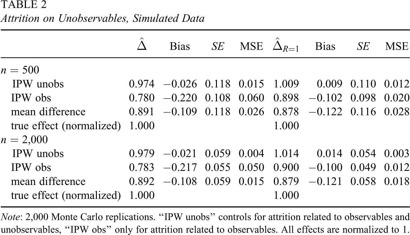
Note: 2,000 Monte Carlo replications. “IPW unobs” controls for attrition related to observables and unobservables, “IPW obs” only for attrition related to observables. All effects are normalized to 1.

Finally, we use a publicly available subsample of Tennessee’s Project STAR Experiment for a simulation study based on empirical data to illustrate the potential gains of IPW when attrition is related to unobservables. The motivation for the use of empirical data is to conduct simulations that are more closely linked to real-world problems with the hope that they are more realistic than studies merely based on generated data. For further examples of simulations that rely on empirical data, see, for instance, Bertrand, Duflo, and Mullainathan (2004), Diamond and Sekhon (2006), Huber, Lechner, and Wunsch (2010), and Lee and Whang (2010).

Project STAR was conducted in the mid-1980s to evaluate the effects of small class sizes (target 13–17 students instead of 22–25 students in regular classes) in kindergartens and schools on student achievement; see, for example, Finn and Achilles (1990, 1999) and Krueger (1999). A major issue for the applicability of the proposed IPW methods under attrition related to unobservables is the requirement of a continuous instrument. Therefore, future experimental designs might consider the inclusion of (close to) continuous instruments that should ideally be randomly assigned in a similar way as the treatment. As mentioned before, the number of phone calls or financial incentives could be used to instrument the response rate to posttreatment surveys. Up to date, however, such variables are typically not available in social experiments and this is also the case for Project STAR. For this reason, we will pursue a somewhat unorthodox simulation approach to investigate the performance of IPW when estimating the ATE on the entire population under attrition related to unobservables.

The original data set that our simulations are based upon contains 6,325 children in kindergarten. We only use those 5,852 observations for which we observe our outcome of interest (Y), namely, the Stanford Achievement Test (SAT) in maths at the end of the kindergarten year (average test score: 485.377, standard deviation: 47.698). From the sample, 1,757 children were randomly assigned to a small class in kindergarten. We discard all treated observations and only keep the sample of controls (n = 4,095), which will serve as the population of interest in the simulations. Moreover, a binary placebo treatment D is randomly assigned among the controls with a “treatment” probability of 0.5. Thus, the true treatment effect is equal to zero as none of the observations was assigned to a small class. Therefore, we know the correct ATE and can determine the bias and MSE in our simulations, despite the use of empirical data.

In a next step, the experiment is artificially broken by the introduction of the following response process, which is designed such that roughly two thirds of the outcomes are observed:

R_{i} = I {β_{0} + β_{1} D_{i} + β_{2} X_{i} - β_{3} Z_{i} - β_{4} U_{i} + V_{i} > 0},

where

β_{0} = 2.5, β_{1} = β_{2} = β_{3} = 1, β_{4} = 2

. X denotes race (one if white and zero otherwise) which we treat as being observed. U represents socioeconomic status (one if eligible for free lunches, zero otherwise) and is assumed not to be observed for the sake of the subsequent simulation. The only generated variables apart from the treatment are the instrument Z (uniform, support [–1.5, 1.5]) and the error term V (standard normal). As a side remark, note that one could also define Z to be an empirical variable that is both continuous and unrelated with Y to even further increase the use of real data. Unfortunately, such a variable is not available in the public use file of Project STAR. An inspection of the data shows that both X and U are strongly correlated with Y. Thus, neglecting attrition supposedly biases estimation. Note, however, that the exact relation between race, socioeconomic status, and the SAT score is unknown due to the use of the empirical data. This is fundamentally different to the conventional Monte Carlo design (see the previous simulations) where the outcome equation is explicitly modeled.

In each of the 2,000 Monte Carlo replications, (Y, X, U) are randomly drawn from the “population” without replacement and (D, Z, V) from their respective distributions in order to compute R. Then, we estimate the response propensity score by regressing R on (1, D, X, Z) and the treatment propensity score, which is unknown in our simulation due to the use of empirical data, by regressing D on $(1, X, \hat{p} (W), X \times \hat{p} (W))$ using probit specifications. Contrary to the previous simulations, we estimate the effects with and without trimming of propensity scores as some values are close to the boundaries. We consider two trimming levels, where response propensity scores smaller than 5% (10%) and treatment propensity scores smaller than 5% (10%) or larger than 95% (90%) are trimmed to the respective threshold values.

Table 3 presents the results which are in line with the previous simulations. The bias of the IPW estimator is moderate irrespective of the sample size and the trimming level, whereas it amounts to roughly 1.8 SAT scores when taking mean differences. Yet, when considering the smaller sample size, the mean difference estimator is superior with respect to the MSE as it is more precise than IPW. However, as the sample size gets larger IPW increasingly outperforms mean differences. We therefore conclude that weighting based on instruments is effective in reestablishing the validity of experiments under attrition on unobservables, at least when the sample size is not too small such that the gain in bias reduction outweighs the loss in precision due to the estimation of the propensity scores and weighting. Of course, a precondition for this result is the availability of a continuous instrument that is both relevant (sufficiently correlated with response behavior) and valid (no direct effect on the outcome). Table 3 also reports the average numbers of trimmed response and treatment propensity scores in the simulations, which are acceptable even under the 10% trimming level.

Table 3.

Attrition on Unobservables, Empirical Data, Zero Treatment Effect

	$\hat{Δ}$	Bias	SE	MSE	Average Number of Trimmed $p, π$
n = 500
IPW unobs (untrimmed) IPW unobs (5% trimming) IPW unobs (10% trimming) mean difference true effect	0.425	0.425	6.197	38.585
	0.428	0.428	6.198	38.594	0.000, 16.191
	0.443	0.443	6.200	38.631	0.452, 46.177
	1.768	1.768	5.420	32.389
	0.000
n = 2,000
IPW unobs (untrimmed) IPW unobs (5% trimming) IPW unobs (10% trimming) mean difference true effect	0.411	0.411	2.994	9.134
	0.412	0.412	2.994	9.137	0.000, 24.315
	0.423	0.423	2.997	9.158	0.012, 142.857
	1.772	1.772	2.667	10.252
	0.000

Note: 2,000 Monte Carlo replications. “IPW unobs” controls for attrition related to observables and unobservables.

In summary, both studies based on simulated and empirical data suggest that IPW becomes increasingly accurate in terms of the MSE and relatively superior to taking mean differences, as the sample size gets larger and given that the correct attrition process is assumed. This is an interesting finding because there exists, as already briefly mentioned, an important difference between the two designs: Parts of the model, for example, the outcome equation, remain unknown when using empirical data. Therefore, it may not be taken for granted that IPW performs equally well in the latter case, because the threat of incorrectly specifying the treatment propensity score remains even when assuming the correct form of attrition. This advocates a flexible specification of the propensity scores and motivates the use of specification tests in the empirical application presented below.

6. Empirical Application

We present an application of Propositions 4 and 5 (attrition related to observables and unobservables) to a labor market policy experiment which was conducted in the United States in the mid-1990s in order to assess the publicly funded Job Corps program. This program (D), which is currently administered by 124 local Job Corps centers throughout the United States, targets young individuals (aged 16–24 years) who have a legal residence in the United States and come from a low-income household (see Schochet, Burghardt, and Glazerman, 2001) for further details. It provides participants with approximately 1,100 hours of vocational training and education as well as with housing, board, and health services over an average duration of roughly 8 months. Here, we use a subset of the experimental data analyzed by Lee (2009), namely, the female sample that includes 4,044 observations.

Suppose that we would like to learn about the ATE on women’s potential log wages (Y) 1 year after program assignment (mean: 1.661; standard deviation: .415). However, we face the problem that wages are only observed for the nonrandom subsample of the 1,454 employed females (R = 1). Economic theory suggests that the latter are likely to differ from the nonworking with respect to unobservables such as motivation and ability. From an econometric perspective, this sample selection problem is equivalent to the attrition problem discussed in Section 4. Furthermore, empirical results (see, for instance, Mulligan & Rubinstein, 2008, among many others) provide strong evidence that socioeconomic characteristics as education, age, race, and labor market experience are important confounders related to both the employment probability and the potential wages. Fortunately, the data set contains information on all of these factors (X) that were measured in the baseline survey at the program assignment. Finally, we require one or more instruments (Z) that plausibly affect the labor supply decision, but have no direct affect on wages. Following the literature (see, for instance, Das et al., 2003), we assume the number of children and parents' education to be valid instruments for employment, at least given the other information in the data.

We use a probit specification (see Appendix H, available online at http://jeb.sagepub.com/supplemental) to estimate the labor supply equation required for the computation of the response propensity score. Interestingly, the treatment coefficient is significantly negative, which points to the prevalence of so-called lock-in effects due to reduced job search effort during program participation. This phenomenon is well documented in the literature (see, for instance, Sianesi, 2004). As expected, education, age, and a favorable labor market history all increase the employment probability. This implies that the working females have better labor market preconditions than the entire sample. Also mother’s education has a positive impact, supposedly through role models, while the coefficient on number of children is negative, albeit not significant. As a model check, we conducted the nonparametric specification test for propensity scores suggested by Shaikh, Simonsen, Vytlacil, and Yildiz (2009). The test yields a p value of .81 and, therefore, does not reject the null hypothesis of a correct specification. In the second step, we regress the treatment on the observed variables X and the response propensity score in order to estimate the treatment propensity score. Again, the specification test does not reject the null at any conventional level.

We estimate the ATEs on the respondents ( $Δ_{R = 1}$ ) and on the entire population (Δ) by the sample analogs of Propositions 4 and 5 and compare them to naively taking mean differences. As in the simulations, we use two trimming levels such that response propensity scores smaller than 5% (10%) and treatment propensity scores smaller than 5% (10%) or larger than 95% (90%) are trimmed to the respective threshold values. Under the first trimming rule, only 1 response and 2 treatment propensity scores are trimmed; under the second rule the respective numbers are 9 and 24. That is, most propensity scores lie well in the interior of the theoretical support. Finally, standard errors are computed based on 1,999 bootstrap replications.

Table 4 shows the results on estimation and inference. The estimates suggest that the program increases the wages of working women on average by 5.5% (which is only borderline significant) and those of the entire population by 6%, irrespective of the trimming level. These effects are up to one third higher than the mean difference of 4.5%. Therefore, the results, which are robust under alternative propensity score specifications not reported here, suggest that the mean difference may be downward biased, albeit the differences in the effects are not statistically significant. In conclusion, the ATEs on the working and on all women are within the range (but rather at the lower end) of those commonly found for an additional year of schooling (see, for instance, Card, 1999). This appears reasonable, given that the scale of the Job Corps program roughly corresponds to a full year in high school, as argued by Lee (2009).

Table 4.

ATE of Training Participation on Log Wage 1 Year Later

Method	Estimate	SE	p-value
IPW unobs (5% trimming): $Δ_{R = 1}$	0.055	0.034	.108
IPW unobs (10% trimming): $Δ_{R = 1}$	0.055	0.033	.090
IPW unobs (5% trimming): $Δ$	0.060	0.028	.031
IPW unobs (10% trimming): $Δ$	0.060	0.028	.034
Mean difference conditional on employment	0.045	0.022	.040

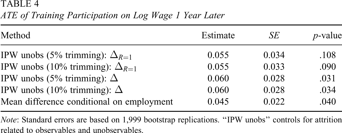
Note: Standard errors are based on 1,999 bootstrap replications. “IPW unobs” controls for attrition related to observables and unobservables.

7. Conclusion

This article discusses the identification of treatment effects in randomized experiments when outcomes are only partially observed due to attrition and nonresponse in follow-up surveys. Its first contribution is the systematic coverage of various forms of attrition, that is, when outcomes are MCAR and when attrition is related to observables (MAR) and unobservables. We treat these various forms by imposing different assumptions on the relation between the response behavior and the treatment, the observed covariates, and the unobserved characteristics in a fairly general treatment effect model.

The second contribution is to show point identification of ATEs on the respondents and on the entire population based on different implementations of IPW. Each IPW method is tailored to the specific nature of attrition considered, which provides practitioners with straightforward solutions depending on the suspected missing data problem. In particular, we introduce an IPW approach based on an IV strategy to tackle attrition on unobservables, which was not considered in the experimental literature before. Our simulation results suggest that an incorrect model for attrition, which, for instance, omits attrition on unobservables, may do worse in terms of bias and MSE than not controlling for the missing outcome problem at all. This highlights the importance of a thorough analysis and correct specification of the response behavior.

Despite its technical ease of implementation, the IV-based IPW approach appears to be rarely applicable in social experiments conducted up to date, due to the lack of credible continuous instruments for attrition. This is unfortunate, as attrition on unobservables seems to be a potential threat in many fields of research where randomized trials are conducted (such as education and labor economics), in particular when the number of observed baseline characteristics is low. For example, in an education experiment, unobserved motivation is likely to be correlated both with the outcome (such as the grade or the test score) and the likelihood to respond (e.g., to participate in a test or exam). Therefore, we argue that future experimental research should seriously consider the creation and random assignment of instruments in order to increase the credibility of experimental inference in the presence of attrition. The number of phone calls in follow-up surveys or financial incentives for responding are just two examples for potentially interesting instruments.

Footnotes

Acknowledgments

The author has benefited from comments by Eva Deuchert, Bernd Fitzenberger, Michael Lechner, Blaise Melly, conference/seminar participants in Freiburg i. B. (research seminar), London (EALE 2010), and Fribourg (SSES 2010), and two anonymous referees.

References

Ahn

Powell

(1993). Semiparametric estimation of censored selection models with a nonparametric selection mechanism. Journal of Econometrics, 58, 3–29.

Angrist

Bettinger

Kremer

(2006). Long-term educational consequence of secondary school vouchers: Evidence from administrative records in Colombia. American Economic Review, 96, 847–862.

Angrist

Lavy

(2009). The effects of high stakes high school achievement awards: Evidence from a randomized trial. The American Economic Review, 99, 1384–1414.

Barnard

Frangakis

C. E.

Hill

J. L.

Rubin

D. B.

(2003). Principal stratification approach to broken randomized experiments: A case study of school choice vouchers in New York City. Journal of the American Statistical Association, 98, 299–311.

Bertrand

Duflo

Mullainathan

(2004). How much should we trust differences-in-differences estimates?. The Quarterly Journal of Economics, 119, 249–275.

Bertrand

Mullainathan

(2004). Are Emily and Greg more employable than Lakisha and Jamal? A field experiment on labor market discrimination. The American Economic Review, 94, 991–1013.

Bloom

Orr

Bell

Cave

Doolittle

Lin

Bos

(1997). The benefits and costs of JTPA title II-A programs: Key findings from the National Job Training Partnership Act study. Journal of Human Resources, 32, 549–576.

Blundell

Powell

(2003). Endogeneity in nonparametric and semiparametric regression models. In Dewatripont

L. H. M.

Turnovsky

(Eds.), Advances in economics and econometrics (pp. 312–357). Cambridge, UK: Cambridge University Press.

Busso

DiNardo

McCrary

(2009a). Finite sample properties of semiparametric estimators of average treatment effects. Working paper, University of California, Berkeley

10.

Busso

DiNardo

McCrary

(2009b). New evidence on the finite sample properties of propensity score matching and reweighting estimators. IZA Discussion Paper No. 3998

11.

Card

(1999). The causal effect of education on earnings. In Ashenfelter

Card

(Eds.), Handbook of labor economics (pp. 1802–1863). Amsterdam, Netherlands: North-Holland.

12.

Castiglioni

Pforr

Krieger

(2008). The effect of incentives on response rates and panel attrition: Results of a controlled experiment. Survey Research Methods, 2, 151–158.

13.

Cochran

W. G.

Chambers

S. P.

(1965). The planning of observational studies of human populations. Journal of the Royal Statistical Society Series A, 128, 234–265.

14.

Crump

R. K.

Hotz

V. J.

Imbens

G. W.

Mitnik

O. A.

(2009). Dealing with limited overlap in estimation of average treatment effects. Biometrika, 96, 187–199.

15.

Das

Newey

W. K.

Vella

(2003). Nonparametric estimation of sample selection models. Review of Economic Studies, 70, 33–58.

16.

Diamond

Sekhon

J. S.

(2006). . In Genetic matching for estimating causal effects: A general multivariate matching method for achieving balance in observational studies. Institute of Governmental Studies Working Paper. University of California, Berkeley.

17.

DiNardo

McCrary

Sanbonmatsu

(2006). . In Constructive proposals for dealing with attrition: An empirical example. Ann Arbor: University of Michigan.. Working paper

18.

Duflo

(2006). Field experiments in development economics. In Blundell

Newey

Persson

(Eds.), Advances in economics and econometrics (Vol. 2, pp. 322–48). New York, NY: Cambridge University Press

19.

Finn

H. D.

Achilles

C. M.

(1999). Tennessee’s class size study: Findings, implications, misconceptions. Educational Evaluation and Policy Analysis, 21, 97–109.

20.

Fisher

(1925). . In Statistical methods for research workers. Edinburgh, UK: Oliver and Boyd.

21.

Fisher

(1935). . In The design of experiments. Edinburgh, UK: Oliver and Boyd.

22.

Fitzgerald

Gottschalk

Moffitt

(1998). An analysis of sample attrition in panel data: The Michigan panel study of income dynamics. The Journal of Human Resources, 33, 251–299.

23.

Frangakis

C. E.

Rubin

D. B.

(2002). The defining role of principal stratification and effects for comparing treatments adjusted for posttreatment variables: From treatment noncompliance to surrogate endpoints. Biometrics, 58, 191–199.

24.

Freedman

(2006). Statistical models for causation: What inferential leverage do they provide. Evaluation Review, 30, 691–713.

25.

Gertler

(2004). Do conditional cash transfers improve child health? Evidence form PROGRESA’s control randomized experiment. The American Economic Review, 94, 336–341.

26.

Grilo

C. M.

Money

Barlow

D. H.

Goddard

A. W.

Gorman

J. M.

Hofmann

S. G.,

… Woods

S. W.

(1998). Pretreatment patient factors predicting attrition from a multicenter randomized controlled treatment study for panic disorder. Comprehensive Psychiatry, 39, 323–332.

27.

Grogger

(2009). Bounding the effects of social experiments: Accounting for attrition in administrative data. mimeo,

28.

Harrison

G. W.

List

J. A.

(2004). Field experiments. Journal of Economic Literature, 42, 1009–1055.

29.

Hausman

J. A.

Wise

D. A.

(1979). Attrition bias in experimental and panel date: The Gary income maintenance experiment. Econometrica, 47, 455–473.

30.

Heckman

J. J.

(1974). Shadow prices, market wages and labor supply. Econometric, 42, 679–694.

31.

Heckman

J. J.

(1976). The common structure of statistical models of truncation, sample selection and limited dependent variables and a simple estimator for such models. Annals of Economic and Social Measurement, 5, 475–492.

32.

Heckman

J. J.

(1979). Sample selection bias as a specification error. Econometrica, 47, 153–161.

33.

Heitjan

D. F.

Basu

(1996). Distinguishing missing at random and missing completely at random. The American Statisticia, 50, 207–213.

34.

Hirano

Imbens

G. W.

Ridder

(2003). Efficient estimation of average treatment effects using the estimated propensity score. Econometrica, 71, 1161–1189.

35.

Horowitz

Manski

C. F.

(1998). Censoring of outcomes and regressors due to survey nonresponse: Identification and estimation using weights and Imputations. Journal of Econometrics, 84, 37–58.

36.

Horowitz

Manski

C. F.

(2000). Nonparametric analysis of randomized experiments with missing covariate and outcome data. Journal of the American Statistical Association, 95, 77–84.

37.

Horvitz

Thompson

(1952). A generalization of sampling without replacement from a finite population. Journal of American Statistical Association, 47, 663–685.

38.

Huber

(2009). . In Treatment evaluation in the presence of sample selection (Department of Economics Discussion Paper no. 2009–07) . Switzerland: University of St. Gallen.

39.

Huber

Lechner

Wunsch

(2010). . In How to control for many covariates? Reliable estimators based on the propensity score. IZA Discussion Paper no. 5268. Institute for the Study of Labor, Bonn, Germany

40.

Imai

(2009). Statistical analysis of randomized experiments with non-ignorable missing binary outcomes: An application to a voting experiment. Journal of the Royal Statistical Society Series C, 58, 83–104.

41.

Imbens

G. W.

(2004). Nonparametric estimation of average treatment effects under exogeneity: A review. The Review of Economics and Statistics, 86, 4–29.

42.

Imbens

G. W.

(2009). Better LATE than nothing: Some Comments on Deaton (2009) and Heckman and Urzua (2009). NBER Working Paper No. 14896. The National Bureau of Economic Research, Cambridge, MA

43.

Imbens

G. W.

Newey

(2009). Identification and estimation of triangular simultaneous equations models without additivity. Econometrica, 77, 1481–1512.

44.

Imbens

G. W.

Wooldridge

J. M.

(2009). Recent developments in the econometrics of program evaluation. Journal of Economic Literature, 47, 5–86.

45.

Karlan

List

J. A.

(2007). Does price matter in charitable giving? Evidence from a large-scale natural field experiment. The American Economic Review, 97, 1774–1793.

46.

Krueger

A. B.

(1999). Experimental estimates of education production functions. Quarterly Journal of Economics, 114, 497–532.

47.

Krueger

A. B.

Zhu

(2004). Another look at the New York City school voucher experiment. American Behavioral Scientist, 47, 658–698.

48.

Lee

D. S.

(2009). Training, wages, and sample selection: Estimating sharp bounds on treatment effects. Review of Economic Studies, 76, 1071–1102.

49.

Lee

Whang

Y.-J.

(2010). Nonparametric tests of conditional treatment effects, . CeMMAP Working Paper CWP36/09. Centre for Microdata Methods and Practice, London, UK

50.

Mealli

Pacini

, (2008). Exploiting instrumental variables in causal inference with nonignorable outcome nonresponse using principal stratification. mimeo

51.

Mulligan

C. B.

Rubinstein

(2008). Selection, investment, and women’s relative wages over time. Quarterly Journal of Economics, 123, 1061–1110.

52.

Newey

W. K.

(2007). Nonparametric continuous/discrete choice models. International Economic Review, 48, 1429–1439.

53.

Newey

W. K.

Powell

J. L.

Vella

(1999). Nonparametric estimation of triangular simultaneous equations models. Econometrica, 67, 565–603.

54.

Neyman

(1923). On the application of probability theory to agricultural experiments. Essay on principles. Statistical Science, Reprint, 5, 463–480.

55.

Robins

Rotnitzky

(1995). Semiparametric efficiency in multivariate regression models with missing data. Journal of American Statistical Association, 90, 122–129.

56.

Robins

Rotnitzky

Zhao

(1995). Analysis of semiparametric regression models for repeated outcomes in the presence of missing data. Journal of American Statistical Association, 90, 106–121.

57.

Robins

Tsiatis

(1991). Correcting for non-compliance in randomized trials using rank-preserving structural failure time models. Communications in Statistics, 20, 2069–2631.

58.

Rosenbaum

P. R.

Rubin

D. B.

(1983). The central role of the propensity score in observational studies for causal effects. Biometrika, 70, 41–55.

59.

Rotnitzky

Robins

(1995). Semiparametric regression estimation in the presence of dependent censoring. Biometrika, 82, 805–820.

60.

Rubin

D. B.

(1974). Estimating causal effects of treatments in randomized and nonrandomized studies. Journal of Educational Psychology, 66, 688–701.

61.

Rubin

D. B.

(1976). Inference and missing data. Biometrika, 63, 581–592.

62.

Rubin

D. B.

(1977). Formalizing subjective notions about the effect of nonrespondents in sample surveys. Journal of the American Statistical Association, 72, 538–543.

63.

Rubin

D. B.

(1978). Multiple imputations in sample surveys—A phenomenological Bayesian approach to nonresponse. In Proceedings of the Survey Research Methods Section, American Statistical Association (pp. 20–34). Alexandria, VA: American Statistical Association.

64.

Rubin

D. B.

(1990). Formal modes of statistical inference for causal effects. Journal of Statistical Planning and Inference, 25, 279–292.

65.

Rubin

D. B.

(1996). Multiple imputation after 18+ Years. Journal of the American Statistical Association, 91, 473–489.

66.

Rubin

D. B.

(2008). For objective causal inference, design trumps analysis. The Annals of Applied Statistics, 2, 808–840.

67.

Scharfstein

D. O.

Rotnitzky

Robins

J. M.

(1999). Adjusting for nonignorable drop-out using semiparametric nonresponse models. Journal of the American Statistical Association, 94, 1096–1120.

68.

Schochet

P. Z.

Burghardt

Glazerman

(2001). . In National Job Corps study: The impacts of Job Corps on participants employment and related outcomes. Report. Washington, DC: Mathematica Policy Research.

69.

Shaikh

A. M.

Simonsen

Vytlacil

E. J.

Yildiz

(2009). A specification test for the propensity score using its distribution conditional on participation. Journal of Econometrics, 151, 33–46.

70.

Sianesi

(2004). An evaluation of the Swedish system of active labour market programs in the 1990s. Review of Economics and Statistics, 86, 133–155.

71.

Wooldridge

(2002). Inverse probability weighted M-estimators for sample selection, attrition and stratification. Portuguese Economic Journal, 1, 141–162.

72.

Wooldridge

(2007). Inverse probability weighted estimation for general missing data problems. Journal of Econometrics, 141, 1281–1301.

73.

Zhang

Rubin

D. B.

(2003). Estimation of causal effects via principal stratification when some outcome are truncated by death. Journal of Educational and Behavioral Statistics, 28, 353–368.

74.

Zhang

Rubin

D. B.

Mealli

(2008). Evaluating the effects of job training programs on wages through principal stratification. In Millimet

Smith

Vytlacil

(Eds.), Advances in econometrics: Modelling and evaluating treatment effects in econometrics (Vol. 21, pp. 117–145). New York, NY: Elsevier Science Ltd.

Supplementary Material

Please find the following supplemental material available below.

For Open Access articles published under a Creative Commons License, all supplemental material carries the same license as the article it is associated with.

For non-Open Access articles published, all supplemental material carries a non-exclusive license, and permission requests for re-use of supplemental material or any part of supplemental material shall be sent directly to the copyright owner as specified in the copyright notice associated with the article.

0.00 MB

0.12 MB