



Abstract
The authors present a generalization of the multiple-group bifactor model that extends the classical bifactor model for categorical outcomes by relaxing the typical assumption of independence of the specific dimensions. In addition to the means and variances of all dimensions, the correlations among the specific dimensions are allowed to differ between groups. By including group-specific difficulty parameters, the model can be used to assess differential item functioning (DIF) for testlet-based tests. The model encompasses various item response models for polytomous data by allowing for different link functions, and it includes testlet and second-order models as special cases. Importantly, by assuming that the testlet dimensions are conditionally independent given the general dimension, the authors show, using a graphical model framework, that the integration over all latent variables can be carried out through a sequence of computations in two-dimensional subspaces, making full-information maximum likelihood estimation feasible for high-dimensional problems and large datasets. The importance of relaxing the orthogonality assumption and allowing for a different covariance structure of the dimensions for each group is demonstrated in the context of the assessment of DIF. Through a simulation study, it is shown that ignoring between-group differences in the structure of the multivariate latent space can result in substantially biased estimates of DIF.
Keywords
Introduction
The bifactor model is an item response theory (IRT) model that accommodates conditional dependencies between items grouped in item clusters by including “specific” dimensions for the clusters, in addition to the “general” dimension. For testlet-based tests, item clusters correspond to testlets (Bradlow, Wainer, & Wang, 1999). If there are

The bifactor structure was first introduced by Holzinger and Swineford (1937) as a special case of confirmatory factor analysis for continuous responses. The model has been extended to item-level analysis for binary data by Gibbons and Hedeker (1992) and for polytomous data by Gibbons et al. (2007). An important contribution of Gibbons and Hedeker (1992) and Gibbons et al. (2007) was the use of full-information maximum likelihood estimation (MLE). By taking advantage of the independence of the dimensions and nonoverlapping item clusters, the dimensionality of the integration can be reduced from
The bifactor model has been found useful in psychological and educational measurement. For instance, Reise, Morizot, and Hays (2007) suggested the bifactor model for checking the dimensionality of measurement instruments. Gibbons et al. (2008) applied the bifactor model to construct item banks and computerized adaptive tests. DeMars (2006) applied the bifactor model to testlet-based tests as an alternative to testlet models. Testlet models (Bradlow et al., 1999; Wainer, Bradlow, and Wang, 2007) are typically used to accommodate local item dependence among groups of items (the testlets) having a common stimulus. In this case, the secondary dimensions are often treated as nuisance dimensions. The bifactor model, on the other hand, tends to be applied when item clusters correspond to different domains so that the secondary dimensions have substantive interpretations. Technically, either model is applicable to tests with item clusters (see, e.g., DeMars, 2006; Li, Bolt, & Fu, 2006a; Rijmen, 2009, 2010). In fact, it has been shown that the bifactor model is a generalization of the testlet model which is equivalent to the second-order model (De la Torre & Song, 2009; Li et al., 2006a; Rijmen, 2009, 2010). There are other approaches that take into account local dependence among items in item response models (e.g., Braeken, Tuerlinckx, & De Boeck, 2007; Ip, 2002, 2010).
In this article, we present a generalization of the multiple-group bifactor model for assessing differential item functioning (DIF) for testlet-based tests. Unlike any previous work on multiple-group bifactor or testlet models, our model relaxes the assumption of complete independence of all (specific and general) dimensions. In our approach, it is only assumed that the specific dimensions are conditionally independent, given the general dimension. Using a graphical model framework, we show that the assumption of conditional independence suffices to reduce the dimensionality of the integration from
Our model allows the means and variances of all dimensions and the correlations among the dimensions to differ between groups. Li et al. (2006a) and Cai, Yang, and Hansen (2011) proposed similar multiple-group testlet and bifactor models, respectively, but assumed independence of the latent variables. For the bifactor model, Fukuhara and Kamata (2011) allowed only the mean of the general dimension to differ between groups, whereas Wang and Wilson (2005) and Wang, Bradlow, Wainer, and Muller (2008) did not allow for any group differences in the latent variable distributions.
Allowing for a different distribution of ability is especially important when it comes to the assessment of DIF. In unidimensional IRT approaches to DIF assessment, it is generally acknowledged that at least the mean of the ability distribution should be allowed to differ between groups to allow for “impact” of group on ability when testing group-by-item interactions. Ainsworth (2007) demonstrated that ignoring group differences in the means of the secondary dimensions in the multiple-group bifactor model can lead to detection of DIF when none exists. In this article, we investigate whether, in addition to the means of the specific dimensions, it is important to allow the mean of the general dimension, the variances of all dimensions, and the correlations among the specific dimensions to differ between groups. We perform a simulation study that shows that our general approach is more appropriate for assessing DIF when group differences in all of these aspects of the latent variable distribution are present. For example, misspecifying the model by assuming uncorrelated dimensions can lead to biased DIF estimation.
Using the graphical model framework, we derive an efficient method for marginal MLE that does not require high-dimensional numerical integration. This method is generally faster than other ML methods and applicable to various settings without regard to the number of dimensions, items and examinees, and the types of item responses. An alternative estimation approach would be the use of Markov chain Monte Carlo techniques. However, these techniques tend to be slow, and it is difficult to monitor convergence to a stationary distribution and to specify vague priors for variance parameters (e.g., Browne & Draper, 2006; Natarajan & Kass, 2000). Contemporary Bayesian approaches to multiple-group bifactor models do not appear to be feasible for very large problems as discussed by Wang et al. (2008) and Sinharay and Dorans (2010). We demonstrate the utility of our efficient approach by applying it to a realistically large dataset from the Progress in International Reading Literacy Study (PIRLS) study with 10 testlets, 126 binary and polytomous items, and over 5,000 examinees.
The rest of this article is organized as follows. We first describe the proposed multiple-group bifactor model and the estimation method. We then discuss methods for DIF assessment for testlet-based tests. In the next section, the performance of our model for assessing DIF will be compared with alternative models in a simulation study. An empirical study follows to illustrate the use of the proposed method for testing DIF in a large-scale assessment. We end with some final remarks.
Proposed Model
In this section, we describe the proposed multiple-group bifactor model and how it can be used for the assessment of DIF. We begin with the multiple-group unidimensional model and then introduce the multiple-group bifactor model.
Multiple-Group Unidimensional DIF Model
Suppose there are

where
We call the first group,
Multiple-Group Bifactor DIF Model
The multiple-group bifactor DIF model is a multidimensional extension of model (1). Suppose there are

where

where
When the mean
Model (3) incorporates the common assumption that all dimensions are independent in the bifactor model. Gibbons and Hedeker (1992) relied on this assumption in their proof that the dimensionality of the integration can be reduced from
We now propose a multiple-group bifactor model that relaxes the assumption of independent dimensions to the assumption that the specific dimensions are conditionally independent, given the general dimension. The idea is to allow the specific dimensions to depend on the standardized general dimension

If
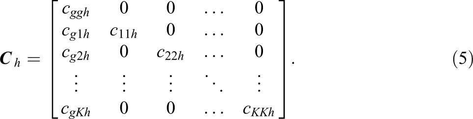
From Equation (5), the covariance matrix
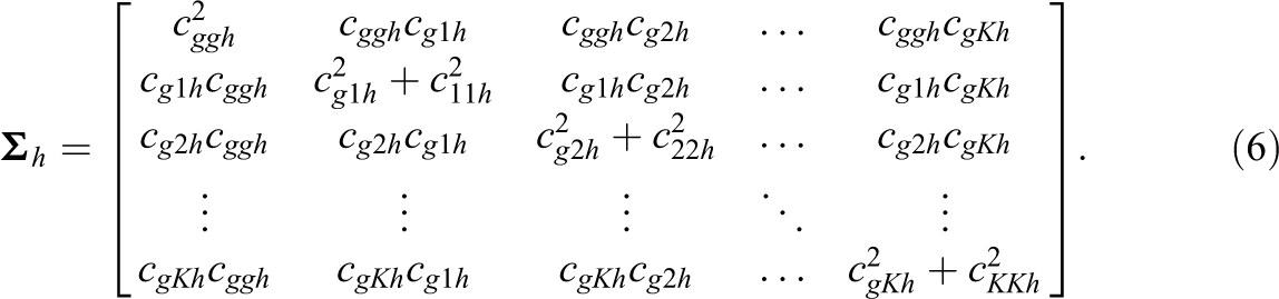
The diagonal elements of
The model is identified by setting the means in the reference group for all dimensions to zero, all variances to one, and all covariances between dimensions to zero,
Returning to binary responses,
Alternative Models
As a comparison to the general approach in Equation (4), we present several models that progressively incorporate stronger assumptions on the equivalence of the ability distributions across groups. All models make the same assumption regarding the conditional response probabilities
The second alternative model takes into account group differences in the general dimension only. This model can be written as

We call Model (7) the multiple-group bifactor “main” model. Finally, we can think of a model assuming no distributional differences in any dimensions,

We call Model (8) the multiple-group bifactor “no impact” model. We also consider two variant models allowing for mean differences between groups in Models (2) and (7) but not for differences in the variances,
Summary of the Six Multiple-Group Bifactor Models According to the Assumptions That Are Relaxed Compared With the “No Impact” Model
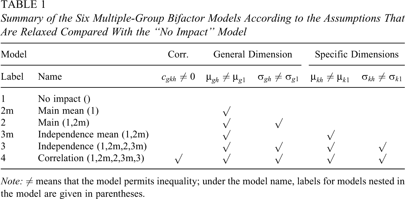
Note: ≠ means that the model permits inequality; under the model name, labels for models nested in the model are given in parentheses.
Estimation
In general, marginal MLE of multidimensional models is computationally very intensive because of the high-dimensional integration over the latent variables. For instance, if Gauss–Hermite quadrature is used to approximate the marginal likelihood function over the latent variables, a
Fortunately, the conditional independence relations that are assumed in the bifactor model can be exploited for MLE. This dimension reduction technique was first described by Gibbons and Hedeker (1992) and used to estimate a single-group bifactor model under the conditions of normally and independently distributed latent variables and for the probit link. The limiting conditions were due to the fact that these authors relied on properties of the multivariate normal distribution. The multiple-group bifactor model by Cai et al. (2011) was based on Gibbons and Hedeker's (1992) formulation.
Glas, Wainer, and Bradlow (2000) derived a marginal ML algorithm for a single-group logistic (3PL) testlet model, which was based on a similar dimension reduction technique to Gibbons and Hedeker (1992). Li, Bolt, and Fu (2006b) presented a multiple-group testlet model based on Glas et al.’s formulation.
All mentioned approaches rely on the assumption that the general and specific dimensions are independent of one another. Using a graphical model framework, Rijmen (2009) showed that the assumption of independently distributed latent variables can be relaxed to conditional independence of the specific dimensions, given the general dimension. In addition, one does not have to rely on properties of the normal distribution, so that the result remains valid under any link function other than the probit function, and for latent variables that are not normally distributed. For the estimation of the multiple-group bifactor model proposed in this article, we use the efficient full-information ML method described in Rijmen (2009).
The method relies on a modification of the expectation–maximization (EM) algorithm. In the E-step of the modified EM algorithm, the graphical model framework is used to perform computations on subsets of variables that are conditionally independent (e.g., Lauritzen, 1995). The M-step proceeds in the same way as the traditional EM algorithm to update parameter estimates. A detailed account of the EM algorithm within a graphical model framework is given in Rijmen, Vansteelandt, and De Boeck (2008). Thus a brief description below will suffice for the purpose of this article.
In the first step, a directed acyclic graph (DAG) is created for the statistical model. The directed graph consists of nodes (variables) and arcs (directed edges; Hunter, Battersby, and Whitehead, 1986) to represent the conditional dependence/independence relations implied in the statistical model (Rijmen et al., 2008). The DAG is then transformed to an undirected graph, called the moral graph. The moral graph can be obtained by adding an undirected edge between all nodes with a common child that are not joined yet and dropping directions from all edges.
Figure 1 illustrates directed graphs and moral graphs for the multiple-group correlation and independence models for person
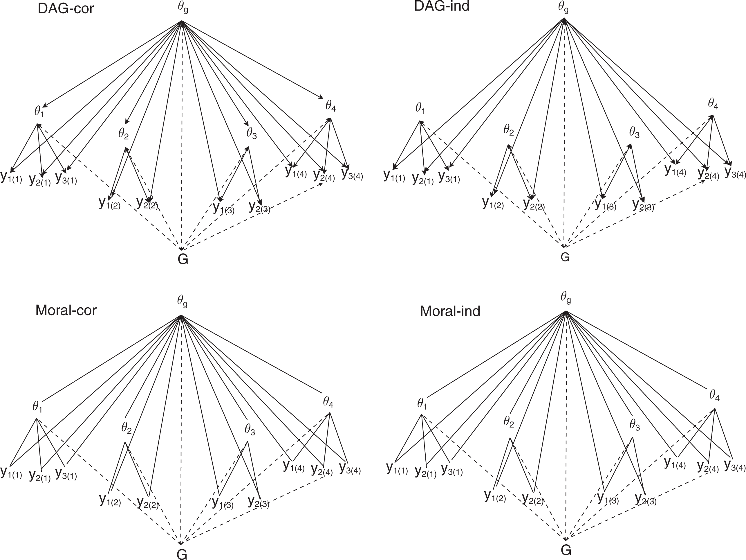
Directed acyclic graphs (DAG) and moral graphs (Moral) for the multiple-group bifactor “correlation” and “independence” models for person j in group h with differential item functioning (DIF) for
In each graph,
In the DAG for the correlation model, there are no direct links between
Most importantly, when transforming the DAG into a moral graph, the same moral graph is obtained for both the correlation and the independence model. The reason is that, for the “independence model,” edges are added between
The moral graph is further transformed into a so-called junction tree. In a junction tree, nodes correspond to sets of variables. The variables in one node are conditionally independent of the variables in another node, given the variables that are in the intersection of both nodes. For the bifactor model, there are
The EM algorithm described in this section was implemented in the Bayesian Networks with Logistic Regression Nodes (BNL) MATBLAB toolbox (Rijmen, 2006). The BNL toolbox can be obtained by contacting the second author.
The EM algorithm does not provide the observed or expected information matrix evaluated at the parameter estimates as a by-product. Hence, standard errors of the parameter estimates are not automatically obtained. Several procedures have been developed to obtain standard errors when using the EM algorithm. An overview can be found in, for example, McLachlan and Krishnan (1997). In BNL, the observed information matrix evaluated at the ML estimates is approximated by the empirical information matrix (Meilijson, 1989). The empirical information matrix is obtained as the sum, over cases, of the outer product of the individual contributions to the gradient of the log-likelihood function.
In order to check for local maxima, a model was run 10 times from relatively diffuse starting values and its log-likelihood and parameter estimates were the same across the multiple runs. We also compared BNL with the ML software PROC NLMIXED in SAS (Wolfinger, 1999) and gllamm (Rabe-Hesketh, Skrondal, & Pickles, 2005) in Stata, and with the Bayesian software WinBUGS (Spiegelhalter, Thomas, Best, & Gilks, 1996) using a small simulated dataset with 12 items, 4 testlets, and 1,000 examinees. The differences in the parameter estimates were mostly negligible between software. In terms of computation time, however, BNL was much faster than other software; for example, for the proposed correlation model, BNL took 20 minutes, SAS took one and a half days, and WinBUGS took one and a half hours for 3,000 iterations and three chains. For the main model, gllamm took 7 hours and BNL 4 minutes. For a simulated dataset with 10,000 examinees, 40 items, and 4 testlets, WinBUGS took nearly 2 days to run 1,000 iterations (three chains), whereas BNL took one and a half hours with 20 quadrature points. Detailed results on this comparison and the code and dataset can be found in the supplementary material provided on the JEBS website (http://jeb.sagepub.com/).
DIF Assessment for Testlet-Based Tests
As we have seen in the previous section, DIF can be modeled as the interaction effect between an item and group membership in an IRT model (e.g., Swaminathan & Rogers, 1990, Swanson, Clauser, Case, Nungester, & Featherman, 2002; Van den Noortgate & De Boeck, 2005). The items for which no interactions are included are called anchor items. If the anchor items include items that show DIF, this will lead to biased parameter estimates (including the DIF effect) for the studied item. An iterative item purification procedure is therefore recommended to ensure that the anchor set does not contain items that show DIF (see e.g., Holland & Thayer, 1988).
For modeling DIF, it is crucial to properly take into account the overall group differences, referred to as “impact” (see e.g., Millsap & Everson, 1993). Otherwise, the DIF effect may merely reflect group differences in the ability distributions, and one would erroneously conclude that an item shows DIF and hence needs further investigation or should even be dropped from the assessment altogether. More seriously, some items that do show DIF may not be flagged and inferences may be biased and thus unfair for certain subgroups.
How to take into account overall differences in the ability distribution depends on the statistical model being in place. For unidimensional IRT models, group differences in the ability distribution are typically taken into account by allowing for a different mean and variance for each group. A similar approach can be followed for multidimensional IRT models including the bifactor model; since the latent space is now multidimensional, group differences in the multidimensional space must be properly taken into account for DIF assessment (for an in-depth discussion, see e.g., Meredith, 1993).
Recently, Wang et al. (2008) presented a DIF assessment method using a Bayesian testlet model. They allowed the studied item’s parameters to differ between two examinee groups, using the rest of the test as the anchor, similarly to the LR approach by Thissen, Steinberg, and Wainer (1988). Unfortunately, Wang et al. (2008) assumed that the ability distributions are the same for the focal and reference groups. Similarly, Fukuhara and Kamata (2011) extended the bifactor model for DIF assessment and estimated it using WinBUGS but allowed only the mean of the general dimension to differ between groups. Furthermore, the methods by Wang et al. (2008) and Fukuhara and Kamata (2011) do not appear to be feasible for practical DIF assessment. For instance, in Wang et al. (2008), assessing DIF in a dataset on 903 examinees took about 3 hours, and Sinharay and Dorans (2010) pointed out that it would take a few days to apply their procedure to a test such as the SAT with nearly half a million students.
In an ML framework, Li et al. (2006b) and Cai et al. (2011) presented the multiple-group testlet and bifactor models, respectively. Ainsworth (2007) presented a similar multiple-group bifactor model viewed as a multiple indicator multiple cause model. However, these models assumed independence of the latent variables. The model we propose encompasses these approaches but is more general in that it allows for any correlation structure among the latent variables that is consistent the conditional independence of the specific dimensions given the general dimension.
Another model-based approach to DIF assessment is the Simultaneous Item Bias Test (SIBTEST; Shealy, 1989; Shealy & Stout, 1991, 1993). The underlying idea of this multidimensional IRT approach is that there are one or more nuisance dimensions that act as a source of bias with regard to inferences concerning the intended dimensions. However, the performance of SIBTEST has not been established yet for testlet-based tests. Lee, Cohen, and Toro (2009) investigated SIBTEST and Poly-SIBTEST for DIF detection in testlets-based tests, and they found that Type I error rates of both tests increase as the sample size increases and the number of items decreases.
Alternatives to model-based approaches are the Mantel–Haenszel (MH) method (Holland & Thayer, 1988) and area measures. The MH method is based on stratifying the sample according to measures of ability (often observed total scores), and testing for associations between item responses and group membership within ability strata. However, for multidimensional tests, the MH method requires that strata be defined by multivariate matching which could be cumbersome and arbitrary (Clauser, Nungester, Mazor, & Ripkey, 1996; Mazor, Kanjee, & Clauser, 1995). Further, this approach involves heavy data requirements because of the need to cross the levels of all variables that go into the match (Dorans & Holland, 1993). For this reason, the logistic regression procedure, regressing item responses on the measures of ability and group, was recommended for DIF analysis for multivariate tests (e.g., Clauser et al., 1996; Mazor et al., 1995). In addition, Wang et al. (2008) showed that the MH method appeared unstable for items with extreme difficulty values. Others have also found that the MH method can be misleading when the true model is a two-parameter model (Bolt & Stout, 1996; DeMars, 2009; Meredith, 1993; Roussos & Stout, 1996).
Area measures can also be used for DIF detection for multidimensional tests (e.g., Raju, 1988). The differential functioning of items and tests (DFIT) procedure of Oshima, Raju, and Flowers (1997) would be an example. This method requires prior estimation of the item response functions (IRFs) for focal and reference groups. The measure of DIF is then a weighted average of squared differences between the estimated focal and reference group IRFs for the studied item. However, as far as we are aware, the performance of the DFIT method for the bifactor model has not been examined yet.
Simulation Study
A simulation study was carried out to examine the performance of the proposed multiple-group bifactor DIF model and to assess the effects of misspecification of the distribution of the latent variables on the estimation of DIF.
Design
We considered a 40-item test composed of four testlets with 10 items within each testlet. We generated data for 10,000 test takers, evenly divided into a focal group and a reference group. There were five conditions corresponding to different specifications of the latent variable distributions. For each of these five specifications, two different DIF sizes for
No impact (1): No distributional differences in any dimension (121 parameters),
Main (2): Differences in the mean and standard deviation of the general dimension only (123 parameters),
Independence (3): Differences in the means and standard deviations of all dimensions, with dimensions that are independent of each other (131 parameters),
Correlation, low (4): Low correlations between the general dimension and the specific dimensions (135 parameters),
Correlations, high (4): Moderate to high correlations between the general dimension and the specific dimensions (135 parameters),
Table 2 lists the true values for the item discrimination parameters in the general and the four testlet-specific dimensions (
True Values for Item Parameters

All six models previously discussed and shown in Table 1 were fitted to the datasets generated under the first four conditions. For the “correlation, high” model, only the three more complex models (independence mean, independence, and correlation) were fitted. The fitted models correspond directly to the generating models, except that two additional models were fitted: the main mean model (2m) with 122 parameters and the independence mean model (3m) with 126 parameters, which are constant-variance versions of the main model (2) and independence model (3), respectively. A given fitted model is misspecified if, looking this model up in Table 1, the generating model is not given in parentheses under the model name. All models were fitted using Gaussian quadrature with 20 quadrature points per dimension. We used a convergence criterion of
Results
We first consider the error (estimated minus true values) for the DIF parameter estimates under each condition. The boxplots in Figures 2 and 3 summarize the results for small and medium–large DIF, respectively.

Boxplots of error (
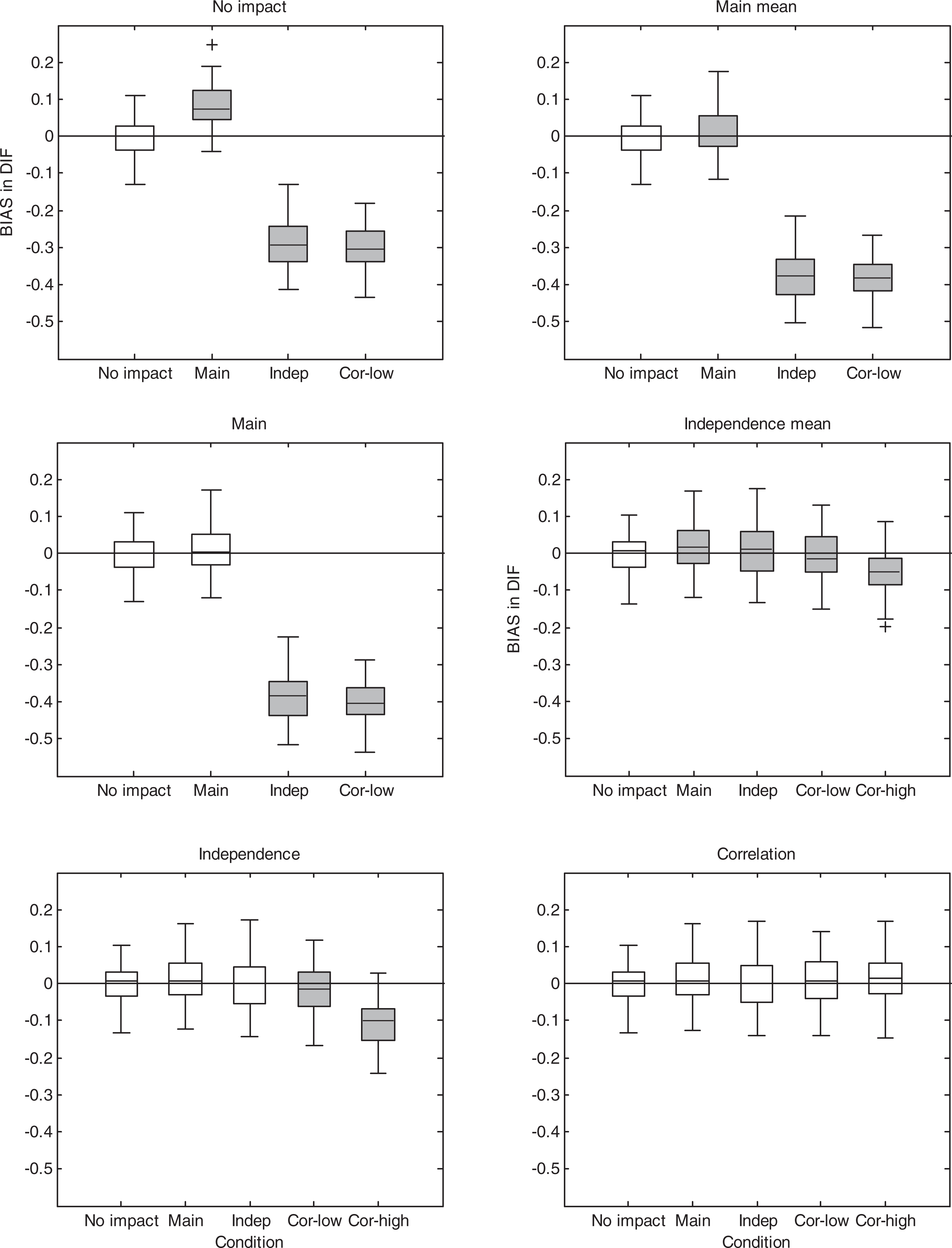
Boxplots of error (
Each panel corresponds to a fitted model, in order of increasing complexity of the models, and each boxplot within a panel corresponds to one of four or five data generating conditions. When the fitted model is misspecified (i.e., the generating model is not nested in the fitted model), the boxplot is shaded.
As expected, the correlation model performs very well in all conditions, showing less error than the misspecified constrained models. Interestingly, for a given generated model, the estimates from the correlation model do not tend to be more variable than those from the more constrained correctly specified models, suggesting that the correlation model could be used as the default model. Assuming equal testlet means (first row of figures) resulted in severe underestimation of the DIF effect when the data were generated from the independence and correlation models because in these models, the testlet mean is
As advocated by Skrondal (2000), we performed a statistical analysis of the simulation results, separately for small and medium–large DIF. For each true model for the two DIF conditions, we treated the differences between the estimated and true DIF parameter for the 50 simulated datasets and three or six fitted models as the response variable and used repeated-measures multivariate analysis of variance (MANOVA) to test the difference in the mean error (i.e., the bias) between fitted models. The overall
Now we discuss bias of the estimates for the other model parameters. To summarize the results for a large number of item parameters, we averaged the absolute values of the estimated bias across items sharing the same true item difficulty (five different values), and similarly for the discrimination parameters for the general dimension (five different values) and specific dimensions (eight different values). Figure 4 shows the results when DIF = 0.2.
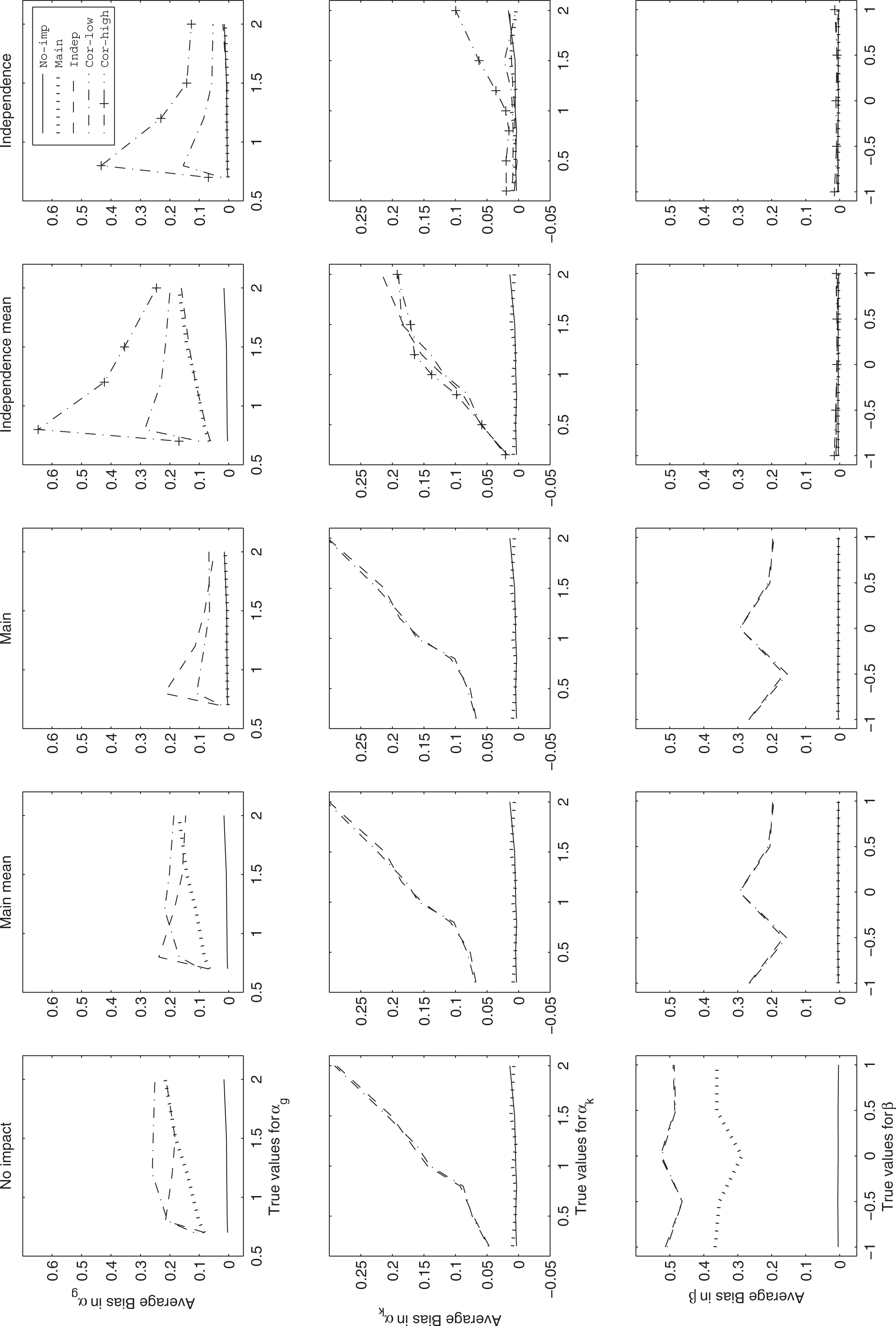
The average of the absolute values of the bias averaged over the items that have the same parameter values for
Each panel represents a fitted model, from the no impact to the independence models. The correlation model is not presented because its bias is negligible in all data-generating conditions. The rows represent the item discrimination parameter for the general dimension (
In general, all fitted models show some degree of bias if the data were generated from a more complex model, except for the difficulty parameters that do not appear to be affected by misspecification of the variances and correlations. Estimates show negligible bias if the data were generated from the same or a less complex model. The pattern of bias differs somewhat between parameters. For
We performed a sequence of LR tests to select among the fitted models for a given simulation condition. To obtain a sequence of nested models, we considered only (from least to most constrained) the correlation, independence, main, and no impact models. The test began by comparing the least constrained (correlation) model with the next, more constrained model in the sequence (independence model); if the test was not rejected, the test proceeded to compare the independence with the main model and finally the main with the no impact model. At the 5% level of significance and when DIF = 0.2, the true model was chosen 90%, 92%, 98%, and 100% of the time under the no impact, main, independence, and correlation models, respectively. A similar pattern was observed under the other DIF condition.
We now present the root mean squared error (RMSE) of the parameter estimates. For simplicity, we computed the average RMSE, as the square root of the average MSE over the 40 items. Figure 5 shows the results when DIF = 0.2.
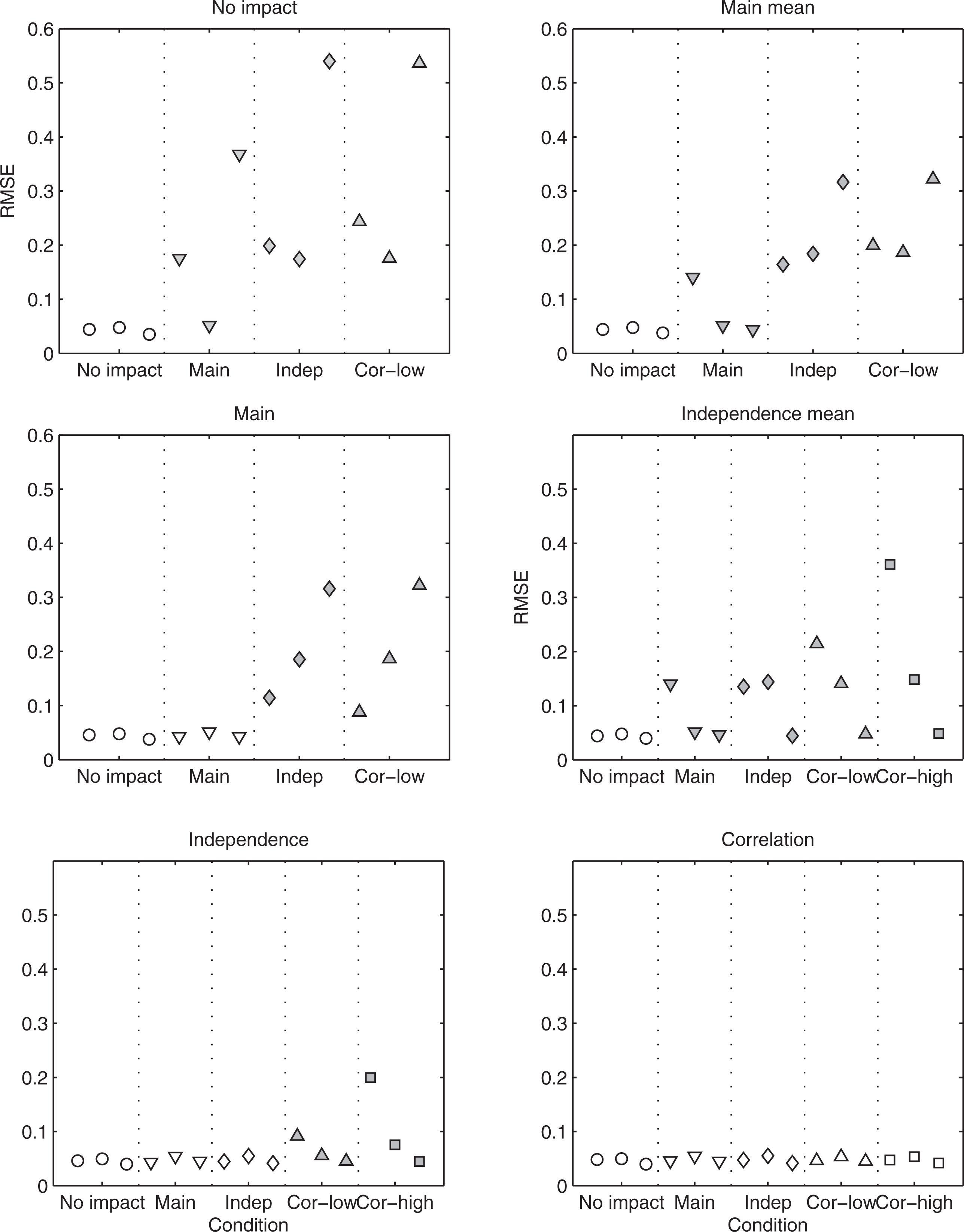
Root mean squared error (RMSE) for the item parameters for the six fitted models, averaged over the 40 items. Panels correspond to fitted models and data-generating models are shown on the x-axis. The parameters are from left to right, the item discrimination parameter for the general dimension (
Each panel corresponds to a fitted model, whereas the generating models are shown on the
Type I Error Rate for DIF Detection
We assessed the Type I error rate of the LR test for DIF detection for the correlation, high model. We generated 200 datasets using the same parameter values as in the simulation study described earlier, except that the DIF parameter was set to zero. We then fitted the correlation model with and without a DIF parameter for Item 37, yielding 13 LR statistics greater than the critical value at the 5% level for a chi-square distribution with 1 degree of freedom. The estimated Type I error rate is therefore 0.065 (=13/200) and this does not differ significantly from the nominal level of
Empirical Study
The multiple-group bifactor model can be applied to large-scale educational assessments such as the National Assessment of Educational Progress, the International Adult Literacy Study, Trends in Mathematics and Science Study, the Programme for International Student Assessment, and the PIRLS. These assessments consist of a large number of testlets, and DIF is of great concern when reporting results for subgroups defined by gender, country, or other variables. In this article, we applied our model to the PIRLS data.
Data and Method
The 2006 U.S. PIRLS data were used to examine gender DIF. There were 5,187 students in total: 2,582 female students (the reference group) and 2,605 male students (the focal group). The assessment consists of 10 passages (testlets), five of which have a literary purpose and five of which have an informational purpose. Each passage is accompanied by 11 to 14 test items. About half of the items are multiple-choice items; the other half are short constructed-response items. There are 126 items in total, 92 binary items and 34 polytomous items (28 items with three categories and 6 items with four categories). The passages and items are distributed across 13 test booklets, and each student responded to the items of one booklet.
We first fitted the correlation model and investigated the covariance structure of the multiple latent traits (one general dimension plus 10 testlet dimensions). We then performed a series of LR tests to determine the most appropriate multiple-group bifactor model for this dataset. Following the procedure that was described in the simulation study, we started with the most general correlation model and simplified it until the reduced model was rejected. Ten quadrature points were used to fit these models. For testing statistical significance of the DIF effect, we used the same kind of LR tests as in the simulation study. Since this required fitting 126 models, we used five quadrature points (for the first 10 binary items, discrepancies between 5 and 10 quadrature points were minor).
Results
Figure 6 shows the estimated means, standard deviations, and correlations for the male students (the focal group) for the 10 testlet-specific dimensions in addition to the general dimension. The horizontal lines at zero represent the value for the female students (the reference group).
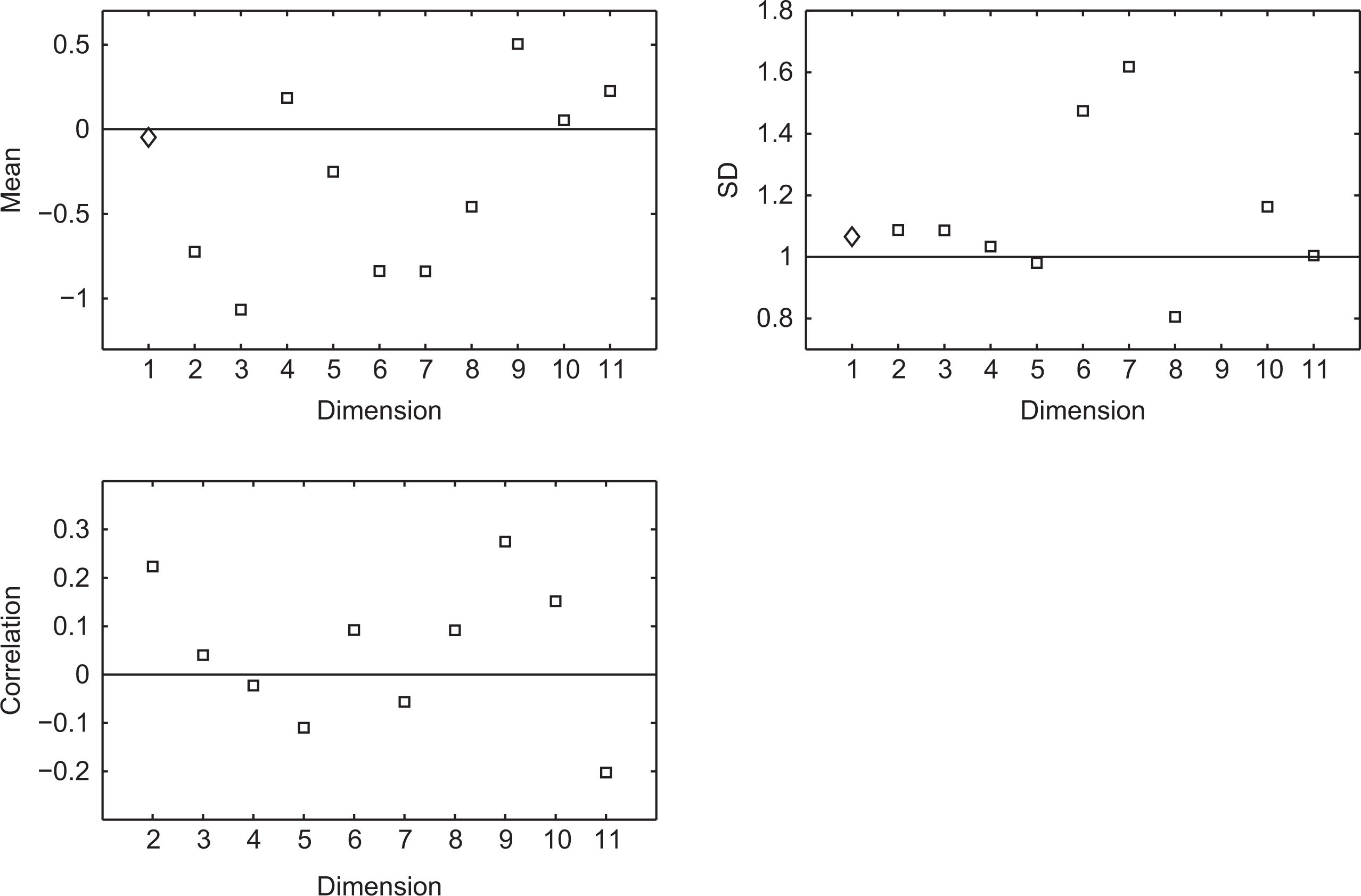
Mean (
The estimated means, standard deviations, and correlations differ somewhat between males and females and across dimensions, with estimated means ranging from −1.06 to 0.5, standard deviations from 0.81 to 1.81, and correlations from
The LR test indicates that the correlation model does not improve upon the independence model (LR = 16.00, df = 10,
DIF was assessed separately for each item, treating the remaining items as anchor items. (Although it was not applied in this study, item purification is highly recommended in practice to find anchor items for detecting DIF for a studied item; see, e.g., Rogers & Swaminathan, 1993; Zumbo, 1999). Figure 7 presents estimates of the DIF parameter for the 91 binary items and 34 polytomous items. Differential item functioning (DIF) estimates for the Progress in International Reading Literacy Study (PIRLS) 2006 data (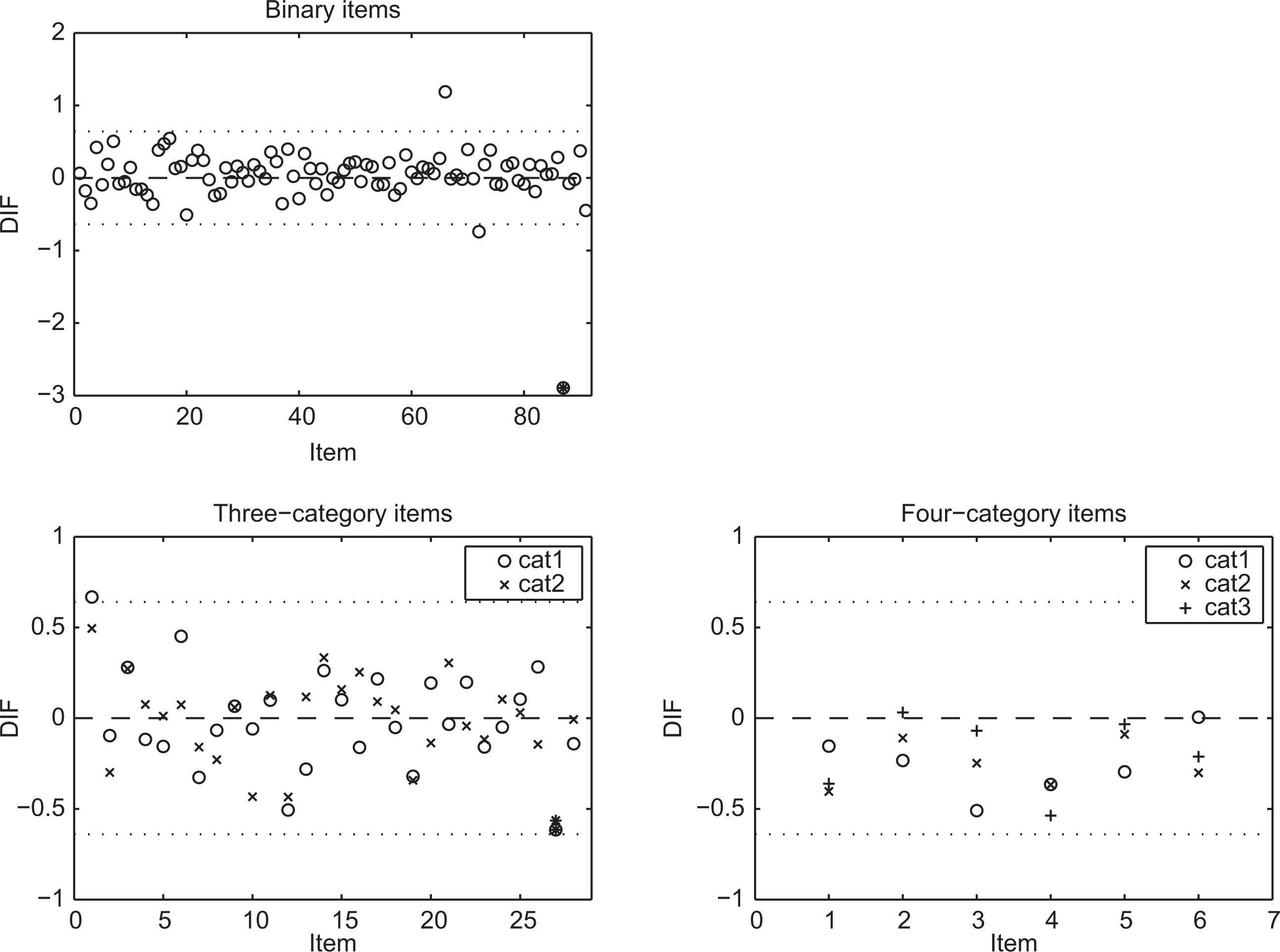
Adjusting the significance level using the Bonferroni correction for multiple comparisons,
Final Remarks
We presented a generalization of the multiple-group bifactor model for assessing DIF for testlet-based tests. The proposed model has four major features: First, it takes into account group differences in the multidimensional latent space. Second, it relaxes the typical assumption that all dimensions are independent to the assumption that the specific dimensions are conditionally independent given the general dimension. Third, the proposed method is flexible and can be applied to various measurement models including testlet and second-order models for binary and polytomous responses. Fourth, the model can be estimated efficiently using a full-information ML method for realistically large problems with many items, testlets, and examinees. Our extensive simulation study shows that ignoring group differences as well as ignoring the correlation structure of the multivariate latent space can result in biased item parameter estimates. In particular, DIF estimates may be substantially biased.
We assumed uniform DIF throughout this article. Nonuniform DIF could be taken into account with an additional parameter, analogous to models for nonuniform DIF in the logistic regression approach (Swaminathan & Rogers, 1990).
The proposed multiple-group bifactor model can also be used to model multidimensionality that is construct-driven. Then, the general factor accounts for the common variance in the constructs being assessed, and the specific factors represent the residual dependencies between items that are assessing the same construct/subconstruct. When the constructs are highly correlated, a testlet or second-order model (which are formally equivalent) may be preferred to the bifactor model.
A few nonmodel-based approaches have been developed for assessing DIF for multidimensional tests (e.g., DFIT). As far as we are currently aware, however, there has been no formal investigation to evaluate the application of such methods to the bifactor models. Future studies will be required to examine their performance on bifactor structures and compare them with the model-based approach that we proposed here.
Footnotes
Declaration of Conflicting Interests
The authors declared no potential conflicts of interest with respect to the research, authorship, and/or publication of this article.
Funding
The authors disclosed receipt of the following financial support for the research, authorship, and/or publication of this article: The research reported here was supported by the Institute of Education Sciences, U.S. Department of Education, through grant R305D110027 to Educational Testing Service. The opinions expressed are those of the authors and do not represent the views of the Institute or the U.S. Department of Education.
References
Supplementary Material
Please find the following supplemental material available below.
For Open Access articles published under a Creative Commons License, all supplemental material carries the same license as the article it is associated with.
For non-Open Access articles published, all supplemental material carries a non-exclusive license, and permission requests for re-use of supplemental material or any part of supplemental material shall be sent directly to the copyright owner as specified in the copyright notice associated with the article.
