
Abstract
Since heterogeneity between reliability coefficients is usually found in reliability generalization studies, moderator analyses constitute a crucial step for that meta-analytic approach. In this study, different procedures for conducting mixed-effects meta-regression analyses were compared. Specifically, four transformation methods for the reliability coefficients, two estimators of the residual between-studies variance, and two methods for testing regression coefficients significance were combined in a Monte Carlo simulation study. The different methods were compared in terms of bias and mean square error (MSE) of the slope estimates, and Type I error and statistical power rates for the slope statistical tests. The results of the simulation study did not vary as a function of the residual variance estimator. All transformation methods provided negatively biased estimates, but both bias and MSE were reasonably small in all cases. In contrast, important differences were found regarding statistical tests, with the method proposed by Knapp and Hartung showing a better adjustment to the nominal significance level and higher power rates than the standard method.
Keywords
Reliability, as the consistency or reproducibility of the test scores (Crocker & Algina, 1986), is one of the most important psychometric properties to be considered when choosing a test for its administration in a specific context. However, reliability, such as it is defined and estimated from the classical test theory, is not a stable property for a given psychometric instrument, but rather a varying characteristic across different applications of the test (Dawis, 1987; Gronlund & Linn, 1990; Pedhazur & Schmelkin, 1991). Thus, in order to obtain a reliability estimate representative enough for future test users, as well as to determine whether one or more factors from the sample characteristics or the administration context have an influence on the reliability of test scores, the best alternative is to quantitatively integrate the reliability coefficients computed with scores from different applications of the instrument under study. And, for carrying out a quantitative synthesis, meta-analysis constitutes an optimal methodological choice (Hedges & Olkin, 1985).
Despite previous meta-analytic studies integrating reliability coefficients that can be found in the literature (e.g., Churchill & Peter, 1984; Conway, Jako, & Goodman, 1995; Parker, 1983; Parker, Hanson, & Hunsley, 1988; Peter & Churchill, 1986; Salgado & Moscoso, 1996; Yarnold & Mueser, 1989), the term reliability generalization (RG) was first proposed by Vacha-Haase (1998). In an RG study, a set of reliability estimates from the same test are integrated, an overall reliability estimate is obtained, and heterogeneity between the individual reliability coefficients is assessed. Moreover, since some heterogeneity across estimates is usually found, a third objective in an RG study consists of looking for moderator variables in order to explain part of that variability.
Although Vacha-Haase’s seminal paper was published just a few years ago, several dozen RG studies have already been carried out. A great variability can be found among these studies in terms of rigor, theoretical underpinning, and methodology. This is partially due to the fact that the RG approach was not conceived as monolithic in terms of the statistical methods applied (Henson & Thompson, 2002; Vacha-Haase, 1998; Vacha-Haase & Thompson, 2011). As a consequence, there is no consensus about several methodological issues affecting the statistical analyses.
One of these issues involves reliability coefficients transformation. Some authors advised to use untransformed reliability coefficients for the statistical analyses (e.g., Bonett, 2010; Henson & Thompson, 2002; Leach, Henson, Odom, & Cagle, 2006; Mason, Allam, & Brannick, 2007; Vacha-Haase, 1998). However, the distribution of the reliability coefficients is skewed for the most usual reliability measures (e.g., α coefficients and Pearson correlations), with a larger asymmetry level as the parameter approximates to one (Rodriguez & Maeda, 2006), as is usually the case for reliability coefficients reported in primary studies. Thus, some other authors recommended applying some transformation on the reliability coefficients in order to normalize their distribution and to stabilize their variances (e.g., Feldt & Charter, 2006; Rodriguez & Maeda, 2006; Sawilowsky, 2000). At least three different transformation formulas have been proposed and/or applied in the RG literature for coefficient α. These alternatives will be examined in more detail further below.
Another issue for which different solutions have been applied so far in the RG approach is the weighting scheme for the reliability coefficients. Some authors just employed ordinary least squares (OLS) analyses in their RG studies, that is, without weighting the reliability coefficients (e.g., Kieffer & Reese, 2002; Leach et al., 2006, Vacha-Haase, 1998). Nonetheless, sample sizes in RG meta-analyses are usually unequal, leading to unequal sampling variances for the reliability coefficients, so that the homoscedasticity assumption—required for OLS techniques—is rarely met (Raudenbush, 1994; Rodriguez & Maeda, 2006). When weights were included in the analyses, some researchers chose the sample size as the weighting factor (e.g., Victorson, Barocas, & Song, 2008; Yin & Fan, 2000; Zangaro & Soeken, 2005), according to the proposal of Hunter and Schmidt (2004), while some others chose the inverse variance of the reliability coefficients (e.g., Aguayo, Vargas, de la Fuente, & Lozano, 2011; Beretvas, Suizzo, Durham, & Yarnell, 2008; López-Pina, Sánchez-Meca, & Rosa-Alcázar, 2009). Inverse variances have been used as the weighting factor in most of the meta-analyses published up to date (Borenstein, Hedges, Higgins, & Rothstein, 2010), and they are also becoming more and more frequent in the RG approach.
When the inverse variance is employed as the weighting scheme, it is necessary to assume some statistical model. One option is to assume a fixed-effect model. The fixed-effect model only considers one source of variation, the within-study variance, which refers to sampling error or the discrepancy between the reliability estimate and the value obtained if the instrument had been applied to the whole target population instead of the limited sample of subjects included in the study. An estimate of the within-study variance is required for the analyses, and several formulae are available for raw reliability coefficients as well as for the different transformations proposed in the literature. This implies that, once the transformation (or no transformation) of the reliability coefficients is chosen, then the estimation method for the sampling variance is unique. The fixed-effect model allows for generalizing results only to the samples whose reliability coefficients were included in the meta-analysis, and also to some external situations where the administration conditions and sample characteristics were identical (Hedges & Vevea, 1998).
An alternative is to assume a random-effects model, which is considered nowadays as the most realistic option in the general meta-analytic arena (Cooper, Hedges, & Valentine, 2009; National Research Council, 1992) and in the RG approach (Rodriguez & Maeda, 2006). The main reason for assuming a random-effects model is that, unlike the fixed-effect one, it allows for generalizing results beyond the studies included in the meta-analysis (Borenstein et al., 2010; Hedges & Vevea, 1998). While the fixed-effect model assumes a constant value for the parametric reliability coefficient across studies, the random-effects model assumes that the integrated reliability coefficients are estimating a random sample of parametric reliability coefficients extracted from a bigger superpopulation. In practice, that implies estimating a second variance component, the between-studies variance. Different procedures are available in the literature for estimating that variance (Viechtbauer, 2005), but no method will provide accurate results unless the number of studies integrated is large enough (Bonett, 2010; Borenstein et al., 2010). Due to the addition of a second variance component, the random-effects model provides more conservative results than the fixed-effect model (Beretvas & Pastor, 2003). Nonetheless, several simulation studies have warned about the limitations of the fixed-effect model in general meta-analysis (e.g., Brockwell & Gordon, 2001; Marín-Martínez & Sánchez-Meca, 2010) and in the RG approach (Bonett, 2010; Romano & Kromrey, 2009).
The random-effects model has also some detractors. Bonett (2010) remarked that the sampling process of reliability coefficients in an RG meta-analysis is usually not random so that, strictly speaking, generalization to a population of reliability coefficients is not appropriate. Instead of the random-effects model, Bonett advocated the use of the varying-coefficient model, first proposed by Laird and Mosteller (1990), where parametric reliability coefficients are allowed to vary between studies but no random sampling is assumed, so that generalization is only intended to the set of primary studies included in the meta-analysis and some others with identical sample and administration conditions.
However, as stated by Laird and Mosteller (1990), “making inferences as if dealing with random samples contrary to fact is not a special issue for meta-analysis, but for all of science and technology” (p. 14). Although the majority of primary research in social, educational, and behavioral sciences is based on nonrandom samples, statistical inference techniques are routinely applied. The reason for this practice is that researchers usually consider their nonrandom samples as reasonably representative of the population to which inferences are intended to be made (Edgington, 1966; Frick, 1998; Overton, 1998). In the same vein, meta-analysts can make inferences to a larger population of studies as long as the set of selected studies can be considered a reasonably representative sample of that population, although the random sampling assumption is not strictly met (Schulze, 2004). Nonrandom sampling is, therefore, a characteristic of research and not specific of meta-analysis: “Rarely in research is the target population of samples fully enumerated and delimited; in fact, data sets used frequently consist of something close to convenience samples” (Schmidt, Oh, & Hayes, 2009, p. 103). The usual aim in meta-analysis, as in any kind of scientific research, is generalization of results and conclusions beyond the sample. In other words, “the goal of science is cumulative knowledge, and cumulative knowledge is generalizable knowledge” (Schmidt et al., 2009, p. 105). The random-effects model allows us for extending our conclusions beyond the set of studies included in the meta-analytic review (National Research Council, 1992). Therefore, the weighting scheme throughout this article will be that based on the inverse variance assuming a random-effects model.
Regarding moderator analyses, it is usually assumed that the predictors included in the model are fixed-effects variables. As a consequence, considering reliability coefficients as a random-effects variable leads to mixed-effects meta-regression models, where some study and sample characteristics are included as predictors of the variability between the reliability estimates. Moderator analyses constitute a crucial step in the RG approach (Rodriguez & Maeda, 2006), given the fact that most of the RG studies published so far found statistically significant relationships of one or more variables to the reliability coefficients. As the psychometric theory predicts, several moderators associated to the variability of test scores have shown a statistically significant relationship with the reliability coefficients in many RG studies (e.g., standard deviation of test scores, type of population from which the sample subjects were recruited), and, for this reason, it has been argued that predictive models of the heterogeneity between reliability coefficients should always include some of them (Botella & Ponte, 2011). Other moderators that have proved a significant relationship with the reliability coefficients in previous RG studies are related to the test version (e.g., test length or original vs. adapted version).
When one or more predictors are included in the model, it becomes necessary to estimate the regression coefficients and, depending on the transformation applied to the reliability coefficients, these estimates will change to some extent. Also a new estimate of the (now residual) between-studies variance, which reflects the amount of heterogeneity on the dependent variable not explained by the moderators incorporated to the model, is required to be included into the weighting factor of mixed-effects analyses. Again, different procedures are available for computing that estimate, and the estimator of choice might have an influence on the results.
Apart from this, statistical tests for the regression model coefficients are required for testing the association of some moderator/moderators with the reliability estimates. The method traditionally computed in mixed-effects meta-analysis for addressing that issue has been criticized in the last few years, since its performance is strongly dependent on the accuracy of the variance estimates (Brockwell & Gordon, 2001). In order to solve that weakness, Knapp and Hartung (2003) proposed a new method based on the addition of a correction factor that takes into account the uncertainty of working with variance estimates instead of with known values. That proposal has not been employed yet in any published RG meta-analysis.
Purpose of This Study
Given the large number of methodological alternatives available when fitting mixed-effects meta-regression models in RG studies, the aim of the present article was to compare the performance of different combinations of methods under some realistic scenarios in RG studies by means of Monte Carlo simulation. Specifically, two estimators of the residual between-studies variance, two methods for testing the significance of the model regression coefficients, and four transformation methods (including untransformed reliability coefficients) were considered, leading to 16 methodological alternatives. Bias and efficiency were studied for the different estimation methods of the model regression coefficients, and Type I error and statistical power rates of their corresponding significance tests were then compared for all methodological combinations. Regarding outcome variables, coefficient α is the most widely reported reliability measure in primary studies and, since mixing different types of reliability coefficients is not appropriate (c.f. Rodriguez & Maeda, 2006), most RG studies published so far have employed coefficient α as the main dependent variable. Thus, this study was focused on α coefficients (transformed or untransformed).
Regarding our hypotheses, we expected that the methods including the Knapp–Hartung correction would perform better than ones combined with the standard method, as reported by the authors in their seminal paper (Knapp & Hartung, 2003). Also, we expected that the transformed methods would outperform the untransformed ones, especially when comparing the Type I error and statistical power rates for the slope tests. Moreover, we expected small variations on the results depending on the residual between-studies variance estimator, as it was previously found (Knapp & Hartung, 2003).
The structure of this article runs as follows: First, the structure of a mixed-effects meta-regression model in the RG approach is sketched; second, the different methods compared in our study are presented; third, a review of previous simulation studies in the RG approach is summarized and then technical specifications of the current study are described; next, the study results are presented; and finally, the results are discussed and some conclusions are provided.
Mixed-Effects Meta-Regression Models in RG Studies
In an RG meta-analysis with k independent studies, let

where
Regression coefficients

Methods for Transforming Coefficients α
According to the classical test theory (Crocker & Algina, 1986), reliability is defined as the quotient between the population variances of the true and observed scores, which can also be expressed as a squared correlation. Since true scores are unknown in practice, some alternative procedure for estimating the scores reliability is needed. Several methods are available nowadays for obtaining a reliability estimate. Since each of these methods is based on different theoretical assumptions, they will provide non-interchangeable reliability measures (Graham, 2006). Therefore, as they estimate different measurement errors, mixing different reliability coefficients in the same meta-analysis is not appropriate. Some of these methods (e.g., test–retest, parallel forms) compute the reliability coefficient as a correlation, so that it seems reasonable to transform these reliability coefficients using Fisher’s Z, which was proposed for normalizing the distribution of Pearson correlations. Conversely, coefficient α is not a correlation, and it remains unclear which consequences should be expected after applying Fisher’s Z transformation to these reliability coefficients.
Table 1 gathers some different options proposed in the RG literature for transforming coefficients α, including the raw α coefficients themselves on the first place. Up to date, when a transformation was applied, Fisher’s Z was the most employed one, although that transformation is theoretically appropriate only when the reliability coefficients are computed as a Pearson correlation, and that is not the case for α coefficients, which constitute the main dependent variable in almost every single RG study carried out so far. For that reason, Rodriguez and Maeda (2006) recommended using a transformation first proposed by Feldt (1969) for two samples and extended by Hakstian and Whalen (1976) for k samples. Finally, another transformation has been proposed more recently by Bonett (2002), in order to compensate for the fact that tests and confidence intervals for α are based on the usually unrealistic assumption that the k parts of the test are parallel. Bonett (2010) proposed to use this transformation on each individual coefficient α when fitting meta-regression models, as it is a variance-stabilizing and approximate normalizing transformation of the coefficient α distribution. In the same vein, Bonett’s transformation can also be applied in the context of mixed-effects meta-regression models when α coefficients constitute the outcome variable. Table 1 provides formulae for computing all three transformations. Also, formulae for their respective sampling variances (
Methods for Transforming Reliability Coefficients
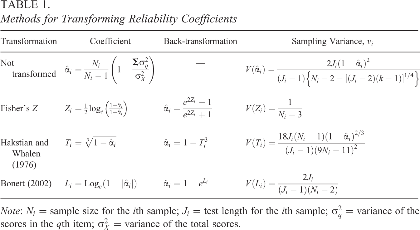
Note:
When some transformation is applied, the statistical results are not directly comparable to those obtained using raw reliability coefficients as the dependent variable (Aguinis, Gottfredson, & Wright, 2011). To account for that issue, equations for back-transformation are gathered in Table 1. These formulae can be applied to mean coefficients α and their confidence limits, the intercept in a regression model, or the mean reliability values for each category in an analysis of variance (ANOVA).
In contrast, to back-transform regression slopes into the original metric, a different strategy is required, given that the value obtained by a simple back transformation of the slope could be misguiding when
Let 
In Equation 3, both the predicted values and the slope are in the metric of the transformation. Our proposal for reporting the slope in the metric of the original reliability coefficient,
Residual Between-Studies Variance Estimators
There are at least seven different procedures for estimating the residual between-studies variance, as a result of extending estimators for the random-effects model (Sánchez-Meca & Marín-Martínez, 2008; Viechtbauer, 2005). In the present article, two estimators will be considered: the extension of the DerSimonian and Laird (DL) estimator and the extended restricted maximum likelihood (REML) estimator.
Extension of the DL estimator
The DL estimator is simple to obtain, since no iterative computation is required. Therefore, it has been the most frequently employed estimator for random-effects meta-analysis not only in the RG approach but also in any application field of meta-analysis. Moreover, it has been included in many different computerized tools developed to help researchers when integrating information from different studies. The extension of this estimator for a mixed-effects meta-regression model with k studies and p predictor variables (see Equation 1) is given by the formula (Raudenbush, 2009):
where

with elements {1/
Extension of the Restricted Maximum Likelihood Estimator (REML)
The REML estimator is a reasonable alternative to the DL procedure just presented. Although it requires iterative computation, this estimator has shown an appropriate performance in previous simulations under a random-effects model for a wide variety of conditions (Viechtbauer, 2005), and has also been recommended by Raudenbush (2009) for mixed-effects models. The estimating process consists of obtaining an adjustment value (a) and adding the previous estimate,
Under a mixed-effects model, with p predictors included in the model (see Equation 1), the adjustment is given by (Raudenbush, 2009):

where
Methods for Testing the Regression Coefficients Significance
The standard method for testing regression coefficients assumes a normal distribution for the regression model coefficient estimates. Despite its wide use in meta-analysis, some authors argued that this method does not take into account the uncertainty of working with estimated variances and that might produce misleading findings (Brockwell & Gordon, 2001; Van Houwelingen, Arends, & Stijnen, 2002). To offset that limitation, Knapp and Hartung (2003) developed a new method by incorporating a correction factor to the traditional formula. Also, their method assumes a t-distribution for the model coefficient values, instead of a normal distribution. Both procedures for testing regression coefficients significance will be presented in this section.
The Standard Method
According to the standard method, the variance–covariance matrix for regression coefficients is obtained with the expression:
with elements {

with
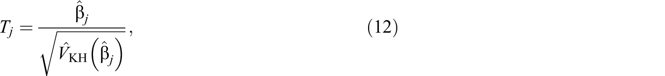
The Knapp–Hartung Method
Knapp and Hartung (2003) proposed the addition of a correction factor to Equation 8 in order to solve the problem mentioned above. Their proposal can be expressed with:
where 
with
In their simulation study, using log-odds ratios as the dependent variable, Knapp and Hartung (2003) found that their new method outperformed the standard one in terms of adjustment to the nominal significance level. Sidik and Jonkman (2005) obtained similar results when comparing both methods. However, the Knapp–Hartung proposal has not been implemented in any RG study yet and, since the dependent variable is different (reliability coefficients), its performance for RG meta-analyses is unknown. Macros for computing both methods have been developed for statistical packages such as R (Viechtbauer, 2010) and Stata (Harbord & Higgins, 2008).
An Illustrative Example
An example is presented here in order to illustrate the 16 resulting methods after combining four alternatives for transforming reliability coefficients, two residual between-studies variance estimators and two methods for testing regression coefficients significance. Data for the example were extracted from an RG study about the Hamilton Rating Scale for Depression (the whole database is available in López-Pina et al., 2009). Considering the samples for which the 17-item version was administered, a meta-regression model was fit using each one of the proposed methods, with the score standard deviation, SD, as the predictor, and the coefficient α,

Slope Estimates and Associated p Values From the Example
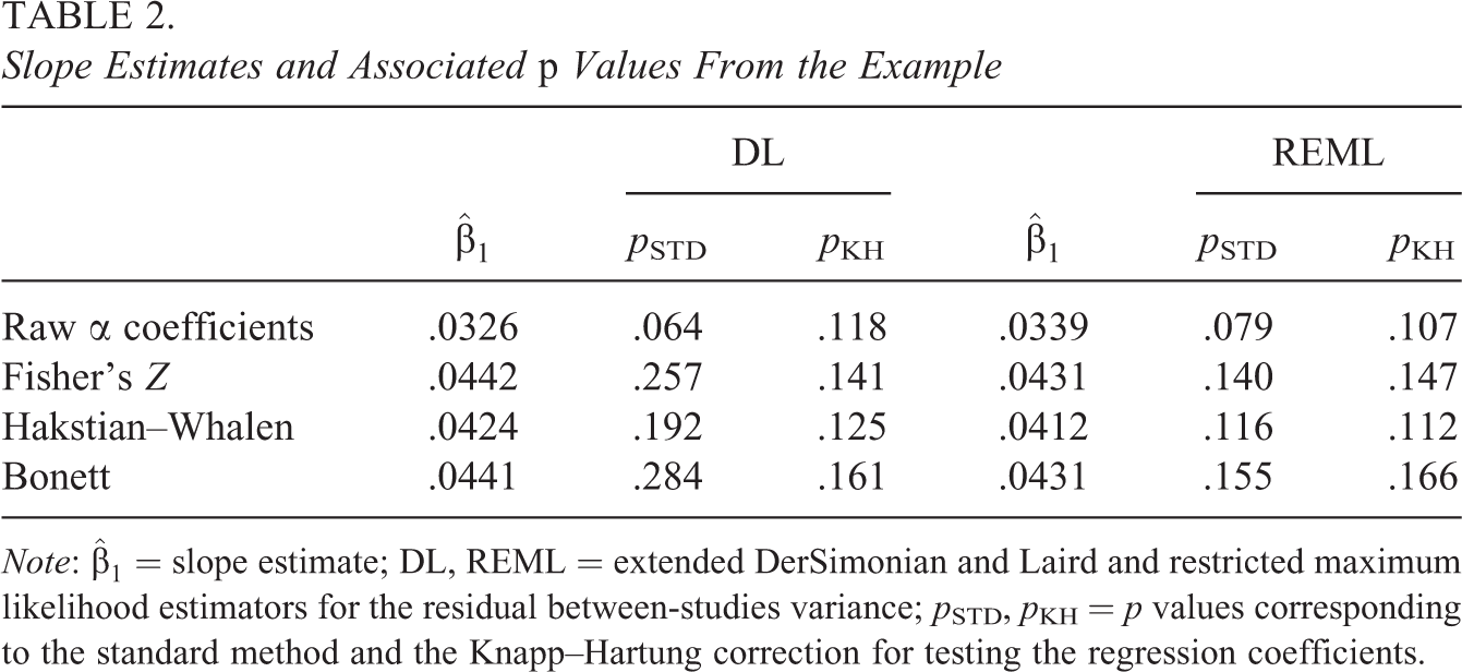
Note:
Regarding the results with the 16 procedures, the slope estimates were around .033 when the raw reliability coefficients were employed as the dependent variable, and values over .04 were obtained when using some transformation. The p values for the slope tests showed important discrepancies depending on the method considered. Assuming a 95% confidence level, statistically significant results were not achieved in any case; however, marginally significant results were found when applying the standard method for testing regression coefficients combined with raw α coefficients, for both DL and REML estimators (p values of .064 and .079, respectively). Conversely, the remaining methods provided p values greater than .10.
Therefore, as data from this example show, the method employed for fitting mixed-effects meta-regression models in the RG approach can affect the results, and that justifies a systematic comparison of the different methodological alternatives in order to determine which method is the most suitable one for a given scenario. In this study, we compared all of the aforementioned methods by means of Monte Carlo simulation. More details about that systematic comparison are provided below.
A Review of Previous Simulation Studies in the RG Approach
The RG approach constitutes a new application field for meta-analysis, and simulation studies are needed to assess the performance of the meta-analytic techniques in this framework, as well as to compare how the methodological alternatives specific to the RG field work under different scenarios. Regarding general meta-analytic methods, Mason et al. (2007) carried out a simulation study comparing the performance of different methods in mixed-effects models. However, the dependent variable in their study was the test–retest correlation instead of the α coefficient. Also, while these authors focused on the efficiency of the different methods included for estimating the model slope, in the present simulation bias, Type I error and statistical power rates were also considered as comparative criteria.
On the other hand, the fact that several transformations are available for the outcome variable is something specific of the RG approach. Feldt and Charter (2006) carried out a simulation study comparing different approaches for averaging internal consistency coefficients, some of them incorporating either the Fisher’s Z or the Hakstian-Whalen transformations. Also, Bonett’s transformation was employed in some recent simulation studies (Bonett, 2010; Romano & Kromrey, 2009). In the present study, all three transformations detailed along this paragraph for the reliability coefficients were included.
Simulation Study
A simulation was carried out to compare the 16 alternative methods for fitting mixed-effects meta-regression models presented above. The simulation was programmed in R, using Metafor (Viechtbauer, 2010) and MCMCpack (Martin, Quinn, & Park, 2011) packages. We decided to conduct this simulation under the classical test theory framework, because most of the tests chosen in previous RG studies were made based on the former.
Regarding manipulated factors in this simulation, sample sizes, Ni
, were generated from a log-normal distribution with a mean value of 150 participants. The asymmetry of the sample size distribution was one of the conditions manipulated, with values of +1, +2, and +3, according to empirical asymmetry values observed in previous RG databases (e.g., Botella, Suero, & Gambara, 2010; López-Pina et al., 2009; Sánchez-Meca et al., 2011). Also, the number of studies for each meta-analysis, k, was set to values of 15, 30, and 60. Finally, for the slope parametric value, two different scenarios were considered: For the first set of conditions, a predictor variable was generated from a distribution N(0, 1) with no relationship to the reliability coefficients, so that the expected value for the slope was 0; for the second scenario, the error component in the test scores was generated as a function of that predictor, leading to a mean empirical slope,
A key aspect in the simulation was the computation of the parametric coefficients α. In a first step, population test scores for each study were generated. Considering settings described in previous simulations (Bonett, 2010; Botella & Suero, 2012), a 20-item test was defined. For the calculation of each parametric coefficient α, a population of 10,000 subjects was defined. True scores for each of the 20 items, tq
, were generated from a multivariate normal distribution with mean 0, variance 2 for each item and covariance 0.4 for any pair of items. This provided a (10,000 × 20) matrix of true scores for each study. Then, error scores for each item, eq, were generated from a normal distribution with mean 0, the variance changing from one study to the next due to the predictor value, with a range between .1 and 1.9. This resulted in another (10,000 × 20) matrix of error scores for each study. The observed scores for each of the 10,000 subjects in the qth item, xsq
, were calculated with the expression (Crocker & Algina, 1986):
Finally, scores for each subject in the whole test were computed as
In a second step, samples of Ni subjects were taken from the respective populations, and the empirical α coefficients, the three proposed transformations, and their respective sampling variances were computed with the formulae gathered in Table 1. This process—generating a database of 10,000 subjects and then extracting a sample of Ni of them—was replicated k times in order to simulate the data corresponding to the k studies in an RG meta-analysis.
Once the sample reliability coefficients and within-study variances for the k studies were obtained, results for each meta-analysis were obtained by fitting mixed-effects meta-regression models for the 16 statistical alternatives under comparison. For each condition, 10,000 meta-analyses were computed.
Regarding comparative criteria, bias and mean square error (MSE) for the slope estimates were first computed in the conditions where
Let 
Then, bias was obtained with:

where

Finally, the proportion of rejections of the null hypothesis
Results
In order to illustrate the general trends of the simulated data, some descriptive statistics are presented in Table 3. Descriptives from the observed scores, xs
, were obtained after generating a database of 1,000,000 scores. Next, data from 1,000 studies were simulated with an asymmetry index of 2 for the sample size distribution, computing for each study the score variance,
Descriptive Statistics From the Simulated Data

Note: xs
= observed total scores for each subject in a population of 1,000,000 participants;
In the remainder of this section, the different methods described above will be assessed by means of the comparative criteria considered in the Monte Carlo simulation. First, accuracy of the slope estimates will be compared for the eight methodological alternatives (after combining four transformation methods and two residual variance estimators), in terms of bias and MSE. Then, performance of the slope statistical tests will be assessed for the 16 available alternatives (as a result of combining the 8 previous methods either with the standard method or with the Knapp–Hartung correction), in terms of Type I error and statistical power rates.
Accuracy of the Slope Estimates
Tables 4 and 5 present bias and MSE results, respectively, for the eight estimators of the meta-regression model slope. In order to facilitate their interpretation, values on both tables were multiplied by 10,000, so that the reference slope value is now 134.8.
Bias in the Slope Estimates for the Different Combinations of Methods
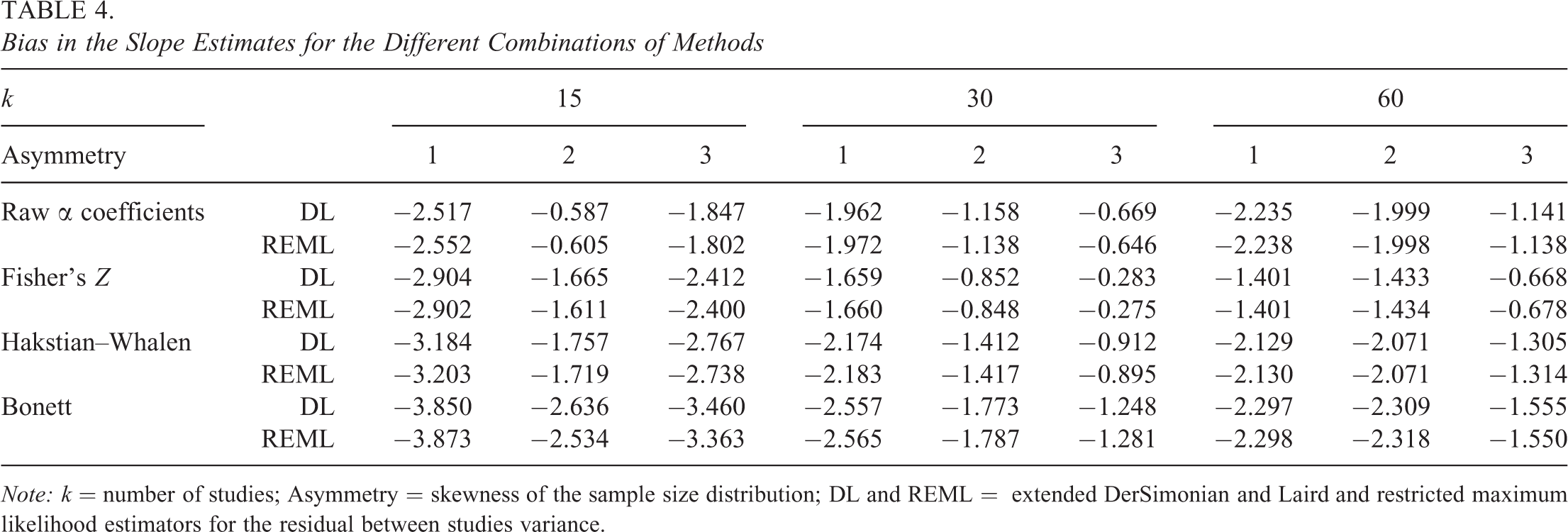
Note: k = number of studies; Asymmetry = skewness of the sample size distribution; DL and REML = extended DerSimonian and Laird and restricted maximum likelihood estimators for the residual between studies variance.
MSE in the Slope Estimates for the Different Combinations of Methods
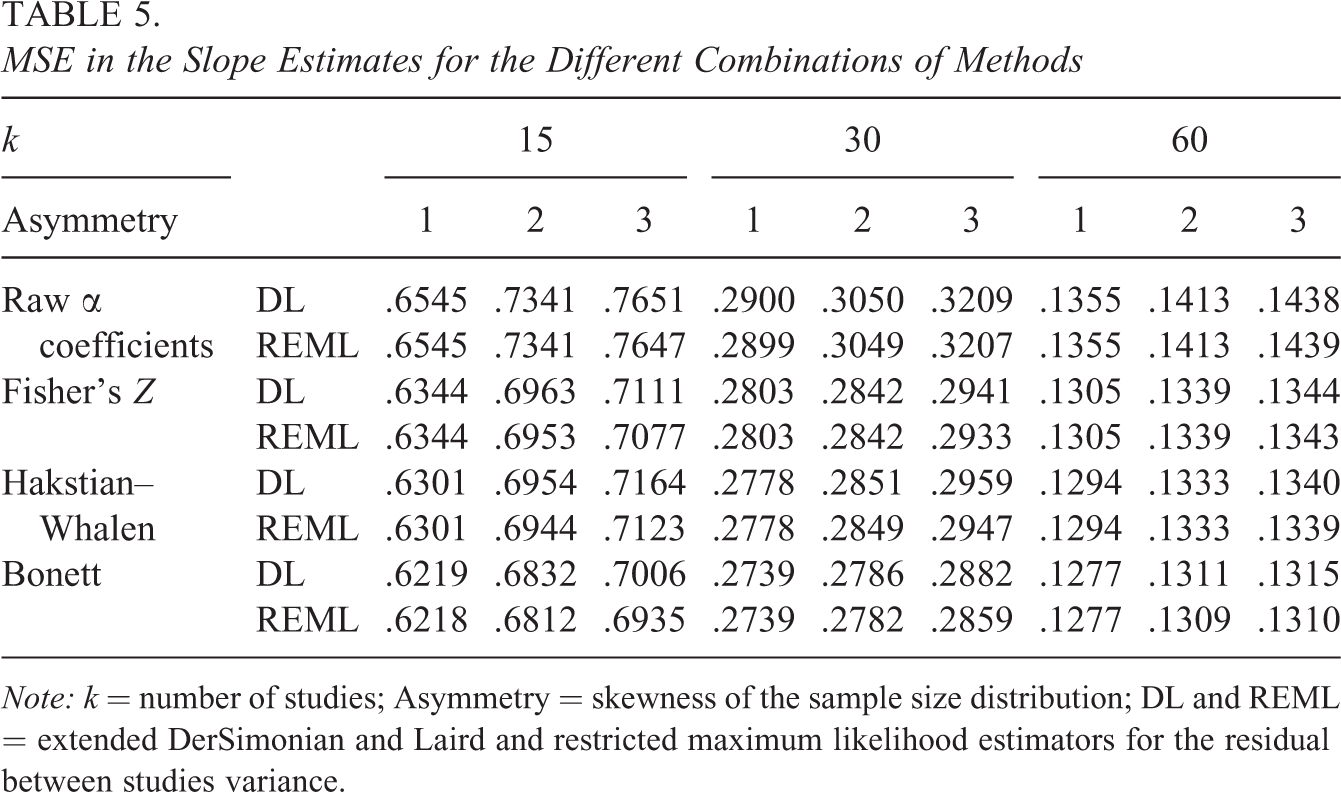
Note: k = number of studies; Asymmetry = skewness of the sample size distribution; DL and REML = extended DerSimonian and Laird and restricted maximum likelihood estimators for the residual between studies variance.
Results in Table 4 show that all conditions provided negatively biased estimates of the slope parameter, although that bias was smaller than 3% for any combination of methods. Results were very similar and showed identical trends regardless of the residual variance estimator, but some differences were observed depending on the transformation method. Specifically, the Bonett transformation systematically showed the highest bias rates, with the largest percentage of bias, around −2.9%, when both the asymmetry in the sample size distribution and the number of studies were small. In contrast, raw α coefficients provided bias results slightly smaller than the methods involving some transformation of the reliability coefficients when the asymmetry was small, while the Fisher transformation led to the smallest bias for larger values in both the asymmetry and the number of studies.
Regarding efficiency, results in Table 5 show some interesting trends as well. MSEs were slightly higher for all the methods as the asymmetry values increased, but the number of studies had a bigger influence decreasing the MSEs for larger k values. Again, results were almost the same for both DL and REML estimators. Focusing on the transformation method, however, raw α coefficients provided the largest MSEs along all of the simulated conditions, while the smallest values were obtained when applying Bonett’s transformation.
Performance of the Slope Statistical Tests
Table 6 gathers Type I error results, while statistical power rates are provided in Table 7. In both tables, only results for the DL estimator are presented, since rates obtained with the REML were very similar and totally comparable in terms of the observed trends.
Type I Error Rates for the Slope Tests Using the DL Estimator

Note: k = number of studies; Asymmetry = skewness of the sample size distribution; STD and KH = standard method and Knapp–Hartung correction for testing the regression coefficients.
Statistical Power Rates for the Slope Tests Using the DL Estimator
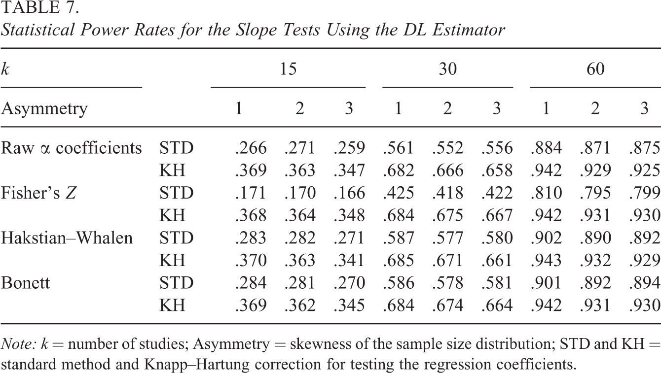
Note: k = number of studies; Asymmetry = skewness of the sample size distribution; STD and KH = standard method and Knapp–Hartung correction for testing the regression coefficients.
Assuming a 95% confidence level, accurate results for each method should be around .05 when the slope parametric value is 0. Results presented in Table 6 show that the rejection rates for the standard method were clearly under the nominal significance level, with rates smaller than .01 for the Fisher transformation and around .02 for the remaining transformation procedures. In contrast, the Knapp–Hartung correction performed close to the nominal level for all of the transformation methods and along all simulated conditions.
Regarding statistical power rates, Table 7 shows that the lowest rates were obtained when combining the standard method and the Fisher transformation. The Knapp–Hartung correction systematically led to higher power rates than those obtained for the standard method. Apart from that, all rates increased for larger k values, while the asymmetry showed a small inverse relationship to the results. Finally, power rates were slightly higher when the Knapp–Hartung correction was combined with some transformation of the α coefficients.
Discussion
The present study was focused on the analyses of continuous moderators by fitting mixed-effects meta-regression models using α coefficients as the outcome variable. Throughout this article, different equations for transforming reliability coefficients, as well as for computing their respective sampling variances and for back-transforming them to the original reliability coefficients metric, were presented (see Table 1). Extensions of the DL and REML estimators for the residual between-studies variance were also detailed (Equations 4 and 6), as well as the standard method for testing the regression coefficients and the adjustment proposed for Knapp and Hartung (2003) to the former (Equations 9 and 12). Performance for all the presented methods was compared by means of Monte Carlo simulation, where bias and MSE for the slope estimates, as well as Type I error and statistical power rates for the slope tests, were the comparative criteria considered.
Out of the different methodological issues implied in the several procedures compared in our article, the choice of the residual between-studies variance estimator (DL vs. REML) produced negligible differences in the trends, the changes observed in the results for the different conditions being very small. On the other hand, the transformation method of the reliability coefficients had some influence on the comparative criteria considered for this study. Finally, the method employed for testing the significance of regression coefficients (standard vs. Knapp–Hartung) showed a critical influence on the Type I error and statistical power results.
Regarding transformations, in terms of bias, all methods provided negatively biased estimates of the regression coefficients, although raw α coefficients showed results slightly better than the ones obtained when applying some transformation, especially when the asymmetry in the sample size distribution was small. Conversely, MSEs were higher for raw reliability coefficients than for any of the transformed methods. However, since bias results were always smaller than 3% regarding the slope parameter, and MSE values were also small and very similar from one method to another, the conclusion should be that all four transformation methods performed reasonably well in terms of bias and efficiency. Also, from a conceptual point of view, Fisher’s Z transformation should not be used with coefficients α, as that transformation is only appropriate when the reliability coefficients were computed as a Pearson correlation coefficient (e.g., test–retest reliability). Therefore, for coefficients α, Hakstian and Whalen’s (1976) and Bonett’s (2002) transformations should be selected.
Considering now the two methods included here for testing the model coefficients, compared to the standard method, the Knapp–Hartung correction provided empirical Type I error rates closer to the nominal significance level, performing almost nominally for all combinations and under all of the simulated scenarios. Regarding statistical power, the Knapp–Hartung correction showed higher rates than the standard method regardless of the rest of conditions manipulated. These power rates were slightly higher when the Knapp–Hartung correction was combined with some transformation of the reliability coefficients. However, a noteworthy finding is that, when integrating 15 or 30 coefficients α, as was the case for some previous RG studies, power rates were considerably lower than the .80 boundary recommended by the scientific community. Thus, having a moderate to large number of reliability coefficients seems to be an important requirement when conducting moderator analyses in RG studies.
Usefulness and Limitations of the Findings Presented in This Article
The simulation study carried out in the presented article showed that, when fitting mixed-effects meta-regression models with one covariate, the slope estimates can be negatively biased, although usually that bias is not large enough to represent a threat for the results. Also, despite the fact that MSEs for these estimates were smaller when some transformation on the reliability coefficients was applied, results were very similar when comparing different transformation methods, and MSEs decreased noticeably as the number of coefficients α increased. Thus, our results suggest that all transformation methods compared here perform similarly in terms of bias and efficiency of the model slope estimates, so that researchers conducting RG studies should pay more attention to some other criteria before making their decisions about the statistical methods implemented.
In contrast to the previous statement, significance tests for the slope did show important differences along the methodological alternatives compared here. According to our results, RG researchers should take into account that testing the model coefficients with the standard method may lead to a loss of statistical power, as Table 7 reflects, so that some moderators of the variability between reliability coefficients might not be identified in their RG studies unless they are integrating a large number of reliability coefficients. The Knapp–Hartung correction outperformed the standard method in terms of statistical power, with rates systematically greater than those obtained with the standard method, and showed Type I error rates closer to the nominal significance level.
Regarding limitations of the methods included in the present study, the fact that only mixed-effects models were considered here might be seen as problematic, since some other options are present in published RG studies. However, the purpose of the present article was not to assess the methodological choices implemented up to date, but rather to compare the best methodological alternatives for future studies, based on the main objectives in an RG study itself and on the current statistical alternatives to accomplish them. Since reliability is not a stable property for a given psychometric instrument (e.g., Crocker & Algina, 1986; Gronlund & Linn, 1990), the RG approach was proposed by Vacha-Haase (1998) as a way to integrate a set of reliability estimates from different applications of a test, and to guide expectations of potential test users about reliability with their sample characteristics and their administration context. That implies generalizing results to some other scenarios not necessarily identical to the ones accounted for in the RG study, and only random-effects models allow researchers for making such generalizations (cf. Beretvas & Pastor, 2003; Borenstein et al., 2010; Hedges & Vevea, 1998; Raudenbush, 2009; Sánchez-Meca, López-López, & López-Pina, in press; Schmidt et al., 2009).
Thus, random-effects models allow for generalizing results beyond the meta-analytic sample of studies and, for that reason, they are considered nowadays as the most suitable option for most meta-analyses (e.g., Cooper et al., 2009; Field, 2003, 2005; National Research Council, 1992; Schmidt, 2010; Schmidt et al., 2009). Note, however, that assuming a random-effects model is only justified if the meta-analyst can consider (on a reasonable basis) the set of studies retrieved for his or her review to be a representative sample of the population to which generalizations are intended. Assuming a random-effects model when conducting moderator analyses leads to mixed-effects models, as the ones presented in this article. In addition to inverse variances, sample sizes can be considered as random-effects weights. However, results are not expected to be influenced by the choice of weights in a random-effects model, but rather by the transformation method in the reliability coefficients (Mason et al., 2007).
Also, as in any simulation, conditions manipulated in our study cannot account for the whole universe of scenarios present in RG studies already carried out or to be done in the future. As an illustration of that, some RG studies have integrated larger numbers of sampling reliability estimates than the ones considered here (e.g., Yin & Fan, 2000), and similar results to the ones presented here for 60 studies should be expected with smaller MSEs and an additional gain of statistical power. Moreover, generating sample size values from a log-normal distribution may be a reasonable approximation to the real situation in many RG meta-analyses (Mason et al., 2007), where most of the primary studies used small-to-moderate inpatient samples while a few ones applied the test as a screening instrument to large samples from general population. Increasing the asymmetry of the sample size distribution produced slightly higher MSEs and smaller statistical power rates, although that factor did not show a big influence on any of the criteria compared here.
Finally, the use of coefficient α in this simulation study, as well as in most of the RG studies published to date, leads to some noteworthy considerations. As Graham (2006) remarked, coefficient α is based on the essentially τ-equivalent measurement model. This implies that, when a coefficient α is computed, it is assumed that all items measure the same latent trait, although probably with a different degree of precision. Researchers estimating reliability with coefficient α, or retrieving α coefficients for carrying out an RG study, must be aware of this assumption, because its violation would directly affect the validity of the reliability estimates for a given test. The generating process of the item scores in our simulation, which was detailed above, fulfilled the requirements of the essentially τ-equivalent measurement model.
The RG approach was recently proposed (Vacha-Haase, 1998), with the aim of applying a methodology for quantitative synthesis, meta-analysis, to the purpose of obtaining a representative reliability value along different administrations of a given test, as well as identifying which factors can explain variability across the set of reliability estimates. The latter objective implies carrying out moderator analyses, and different alternatives for addressing that issue are available to the meta-analyst. Results of this study mainly suggest that, when a mixed-effects model is assumed for the moderator analyses in an RG study, the Knapp–Hartung correction for the statistical test of the model coefficients provides rates closer to the nominal significance level regarding Type I error, and higher power rates than the ones obtained for the standard method. Performance for that correction seems then promising in the RG approach, where it has not been applied to date.
Footnotes
Funding
The authors disclosed receipt of the following financial support for the research and/or authorship of this article: This research was supported by a grant for junior researchers from Fundación Séneca, Region of Murcia, Spain, and by the Ministerio de Ciencia e Innovación, Spanish Government, Project No. PSI2009-12172.