Speededness and Adaptive Testing

Abstract

Two simple constraints on the item parameters in a response–time model are proposed to control the speededness of an adaptive test. As the constraints are additive, they can easily be included in the constraint set for a shadow-test approach (STA) to adaptive testing. Alternatively, a simple heuristic is presented to control speededness in plain adaptive testing without any constraints. Both types of control are easy to implement and do not require any other real-time parameter estimation during the test than the regular update of the test taker’s ability estimate. Evaluation of the two approaches using simulated adaptive testing showed that the STA was especially effective. It guaranteed testing times that differed less than 10 seconds from a reference test across a variety of conditions.

Keywords

adaptive testing Luecht heuristic lognormal response–time model mixed integer programming shadow-test approach test speededness

Introduction

Adaptive tests are typically organized as fixed-length tests with test takers signing up for fixed time slots. However, the items in the pool may show considerable variation in the time they require to process all their information and find a solution. As different test takers get different selections of items from the pool, the time they need to reply to their selection may also vary considerably, with serious differential speededness of the test as a result. Because the time intensity of the items typically correlates with their difficulty, and the difficulty of the selected items correlates highly with the ability of the test takers, usually the more able test takers experience much greater time pressure during adaptive testing than their less able counterparts. Empirical evidence demonstrating this counterintuitive result has been presented, for instance, by Bridgeman and Cline (2003) and van der Linden (2009a).

A method for the control of speededness in adaptive testing was presented by van der Linden (2009a). The method was based on the same response–time (RT) model as in the current study (which will be reviewed below). It consisted of the following components: (a) use of the RTs to permanently update an estimate of the test taker’s speed during the adaptive test; (b) use of the speed estimate along with the estimates of the time intensities for the remaining items in the pool to predict the time necessary for each of them; and (c) selection of the items in the adaptive test subject to a constraint on their predicted times that guarantees completion of the test within the remaining time. Bayesian methodology was used for updating both the estimate of the speed parameter and the predicted times for the test taker on the remaining items in the pool in the method.

Two major differences exist between this earlier study and the method presented in this article. First, the control in the earlier study was one sided in that it only imposed the time limit as an upper bound on the completion time for the test but did not prevent test takers from finishing too early. In fact, because of the low time intensity of the majority of items selected by the adaptive algorithm, the evaluation of the method showed many test takers who actually did finish much earlier (van der Linden, 2009a, figure 1). The new method is designed to offer two-sided control; it prevents candidates from running out of time but at the same time selects combinations of items that imply full use of the time available for the test. We believe this additional feature is important because it allows for more effective scheduling of test takers across the fixed time slots typically used in adaptive tests (no idle testing stations or unrest created by test takers leaving early).

Figure 1.

Plot of the total-time distributions on the reference test for test takers working at speed τ = −.70, −35, 0, .35, and .70.

Second, the new method does not require any real-time estimation of speed parameters for the test takers nor any updating of the predicted distributions of the time the test takers would spend on each of the remaining items in the pool. It thus entirely avoids the computational burden involved in the use of a Bayesian predictive methodology during adaptive testing and produces results not liable to any errors in the estimates of these parameters and distributions. Instead, the new method imposes two simple constraints on the RT parameters of the items that are selected. Consequently, the method is effective directly from the beginning of the test; we do not have to wait for stabilization of any parameter estimates more toward the end of it.

Another key element of the new method is its direct focus on the probability of a test taker running out of time on the adaptive test. Following van der Linden (2011a), the probability is defined as follows: Let $T_{i}$ denote the random response time by a test taker on the items $i =$ $1, . . ., n$ in the test. The total time for the test taker is $T_{t o t} = \sum_{i = 1}^{n} T_{i}$ . Observe that $T_{t o t}$ is random as well; its cumulative distribution function is denoted as $F_{T_{t o t}} (t)$ . Hence, the probability (or risk) of the test taker running out of time is

\begin{array}{c} π = Pr \{\sum_{i = 1}^{n} T_{i} > t_{l i m} | τ, α, β\} \\ = 1 - F_{T_{t o t}} (t_{l i m} | τ, α, β), \end{array}

where τ is the test taker’s speed, $β = (β_{1}, . . ., β_{n})$ is the vector of parameters for the time intensities of the items in the test, and $α = (α_{1}, . . ., α_{n})$ is the vector of discrimination parameters for the items in the response–time model in Equation 2 given below. Notice that the lower the risk, the less stringent the time limit will be. Also, as follows from the RT model below, the risk will be lower for test takers who operate faster, but it will be higher for selections of items that are more time intensive. Each of these relationships makes intuitive sense.

For a given test taker, the probability of running out of time in Equation 1 can be controlled by constraining the vectors α and β for the selection of items in the adaptive test. The same principle was applied in van der Linden (2011b) to assemble fixed test forms to be equally speeded as a reference form, fixed forms with the same degree of speededness but some of the other test specifications changed, as well as the problem of adjusting the degree of speededness of a testing program with a fixed time slot to a newly selected level. As demonstrated below, application of the principle to adaptive testing becomes extremely straightforward for a direct approximation to the distribution function in Equation 1, which leads to two constraints each to be imposed on a simple sum of item parameters. The only thing we need to do during adaptive testing is updating the sums for the items selected in the test.

Total-Time Distribution

The response time for a test taker with speed $τ \in (- \infty, \infty)$ on item i is modeled using the lognormal density

f_{T_{i}} (t; τ, α_{i}, β_{i}) = \frac{α_{i}}{t_{i} \sqrt{2 π}} exp \{- \frac{1}{2} {[α_{i} (ln t_{i} - (β_{i} - τ))]}^{2}\},

with parameters $β_{i} \in (- \infty, \infty)$ for the time intensity or amount of labor required by item i and $α_{i} \in (0, \infty)$ for its discriminating power. The model follows directly from a fundamental equation for response-time modeling derived from the definition of speed on a test as the rate of change in the amount of labor performed on the items with respect to time (van der Linden, 2009b). Bayesian estimation of the parameters with Gibbs sampling from their posterior distributions is described in van der Linden (2006). Alternatively, the item parameters can be estimated using confirmatory factor analysis (Finger & Chuah, 2009). For various methods of checking the fit of the model (Bayesian predictive checks; the deviance information criterion [DIC]; Bayes factors; Bayesian residuals), see Klein Entink, Fox, and van der Linden (2009), and van der Linden (2006, 2007). Throughout this article, we assume that the fit of the model in Equation 2 has been checked carefully with satisfactory results and its parameters have been previously estimated with enough precision to treat them as known.

The density of the distribution of the total time for a test taker with speed τ on two items follows from Equation 2 as

f_{T_{t o t}} (t; τ, α, β) = \int f_{T_{1}} (z; τ, α_{1}, β_{1}) f_{T_{2}} (t - z; τ, α_{2}, β_{2}) d z,

an expression known as the convolution integral of the separate densities for the two items. Repeated application of the integral, each time adding an extra item to the test, gives the distribution of $T_{t o t}$ as the n-fold convolution of the densities for the item distributions. The convolution does not have any known closed form, and its integrals are numerically intractable, even for the case of a test consisting of only a few test items. However, as shown in van der Linden (2011a), it can be approximated excellently by a standard lognormal density using Fenton’s (1960) method of matching the first two cumulants. We only summarize the approximation here; for its derivation as well as examples illustrating its extremely accurate fit, see van der Linden (2011a).

We reparameterize the RT model in Equation 2 and define new item parameters

q_{i} \equiv exp (β_{i} + α_{i}^{- 2} / 2),

and

r_{i} \equiv exp (2 β_{i} + α_{i}^{- 2}) [exp (α_{i}^{- 2}) - 1] .

As a result, although the distribution of $T_{t o t}$ has an unknown shape, its mean and variance can be shown to be equal to

M e a n (T_{t o t}) = exp (- τ) \sum_{i = 1}^{n} q_{i}

and

V a r (T_{t o t}) = exp (- 2 τ) \sum_{i = 1}^{n} r_{i} .

(van der Linden, 2011a, equations 20–21).

The standard family of lognormal distributions family has density

f (x; μ, σ^{2}) = \frac{1}{x σ \sqrt{2 π}} exp \{- \frac{1}{2} {(\frac{ln x - μ}{σ})}^{2}\}, μ, σ > 0.

with parameters μ and σ². The member we need to approximate the density of $T_{t o t}$ has parameters μ and σ² that can be shown to follow from the new parameters in Equations 4 and 5 as

μ = - τ + ln (\sum_{i = 1}^{n} q_{i}) - ln (\frac{\sum_{i = 1}^{n} r_{i}}{[\sum_{i = 1}^{n} q_{i}]^{2}} + 1) / 2,

and

σ^{2} = ln (\frac{\sum_{i = 1}^{n} r_{i}}{[\sum_{i = 1}^{n} q_{i}]^{2}} + 1) .

Observe that μ and σ² are not the mean and variance of the (otherwise unknown) distribution of $T_{t o t}$ in Equations 6 and 7. Rather, as revealed by the parameter structure of Equation 8, they are the equivalent of the mean and variance of the normal distribution of an arbitrary variate ln X. However, substitution of Equations 9 and 10 into 8 gives us its member with the same mean and variance as the distribution of $T_{t o t}$ in Equations 6 and 7.

Controlling Speededness in Adaptive Testing

A surprisingly useful feature of Equations 6 and 7 is their factorization into two parts depending exclusively on the test taker and the item parameters, respectively. The factorization guarantees that, whatever the speed τ of the test taker, the mean and variance of his or her total-time distribution on any two test forms with matching sums of these item parameters are identical. In fact, Equations 8 through 10 show that the same principle holds for the entire shape of the approximating distribution; for any τ, identical sums of $q_{i}$ and $r_{i}$ parameters guarantee identical distributions of $ln T_{t o t}$ , and thus of $T_{t o t}$ .

Another useful feature of each expression in Equations 7 and 8 is that they are based only on sums of the $q_{i}$ and $r_{i}$ parameters. The additivity is particularly convenient in adaptive testing. It allows us to immediately evaluate the impact of any extra item on the properties of the total-time distribution; the only thing we need to do is add the $q_{i}$ and $r_{i}$ parameters for the candidate item to the two sums.

In order to control the speededness of an adaptive test, our basic idea is to identify a reference form with a proven, excellent level of test speededness, and build the adaptive test to produce the same level. For instance, the reference form could be a fixed form used before a program became adaptive or the set of items in a previous adaptive test. It is essential that the actual total times on it have been checked for test takers working at a realistic range of speed and that they have been found to be all right, given the current time limit. In addition, an evaluation of the subjective time pressure experienced by the test takers during the test may play a role. Observe that we only have to check these data for a realistic range of τ values. As for any two matching sums of $q_{i}$ and $r_{i}$ parameters, the conditional distributions of $T_{t o t}$ given τ are automatically identical for each value of τ, differences between the distributions of τ in the populations of test takers for the reference and new forms do not matter.

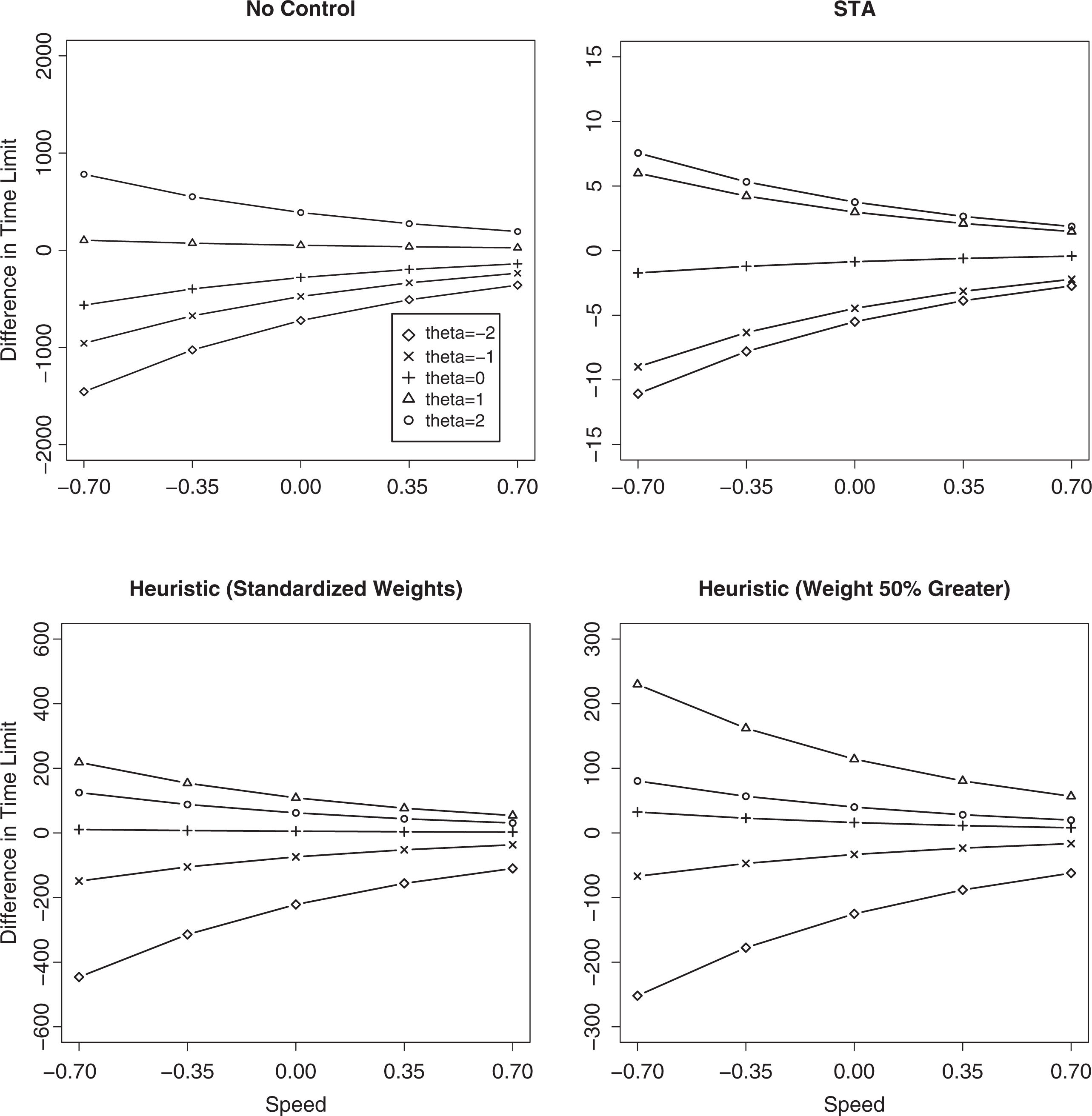
In fact, as the two sums of the $q_{i}$ and $r_{i}$ parameters are the only things we need from the reference test, we could just as well select a priori values for them that are plausible for a test of the intended length, study the degree of speededness in Equation 1 associated with them (for instance, using the risk curves in van der Linden, 2011a, figure 2), modify their values if necessary, and use the final result to set the target values in Equations 11 and 12 below.

Figure 2.

a. Average difference between the time limits for the reference and adaptive tests for the conditions with no control, shadow-test approach (STA), and two versions of the heuristic in seconds (π = .05).

Figure 2.

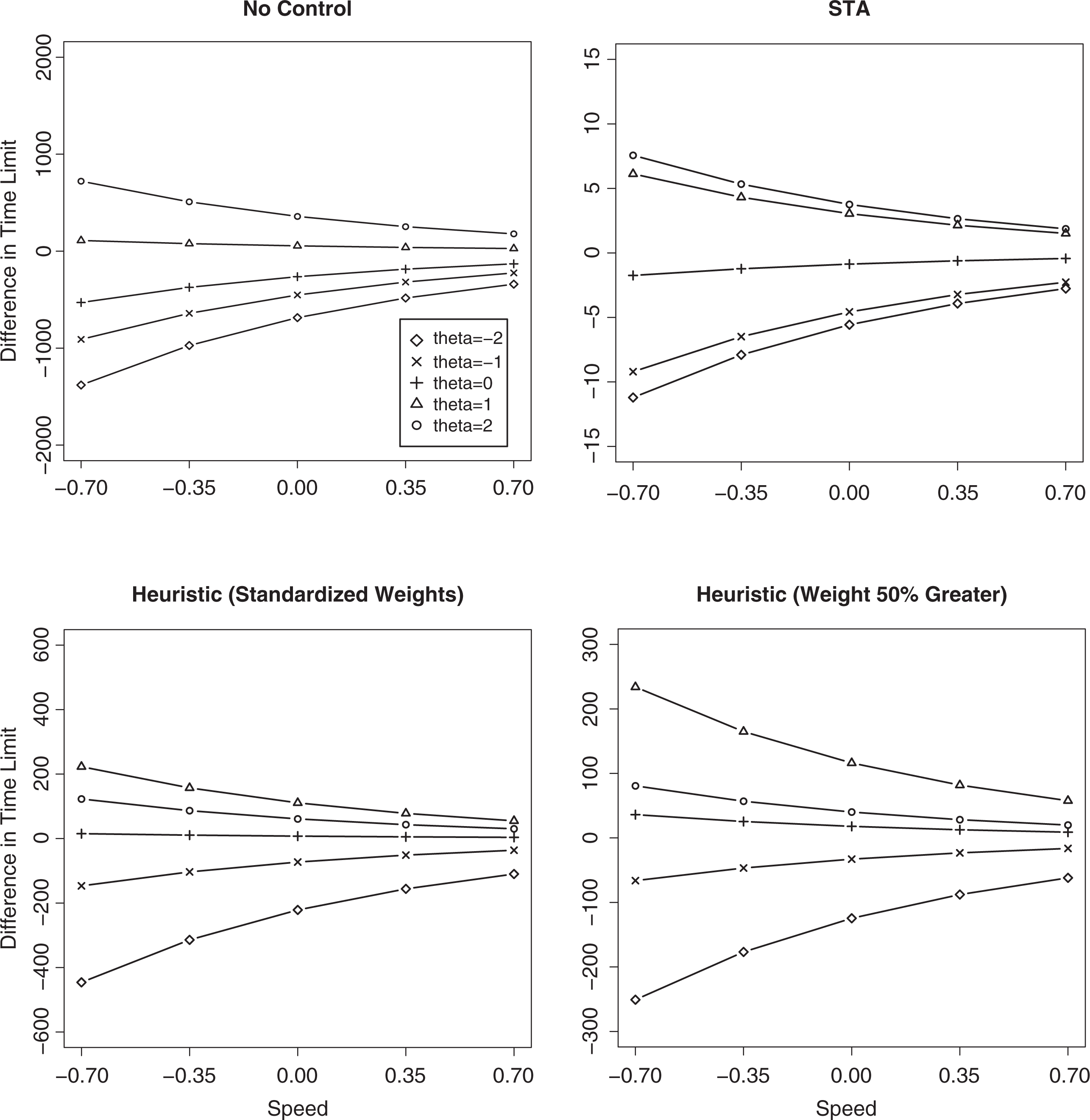
b. Average difference between the time limits for the reference and adaptive tests for the conditions with no control, STA, and two versions of the heuristic in seconds (π = .10).

Figure 2.

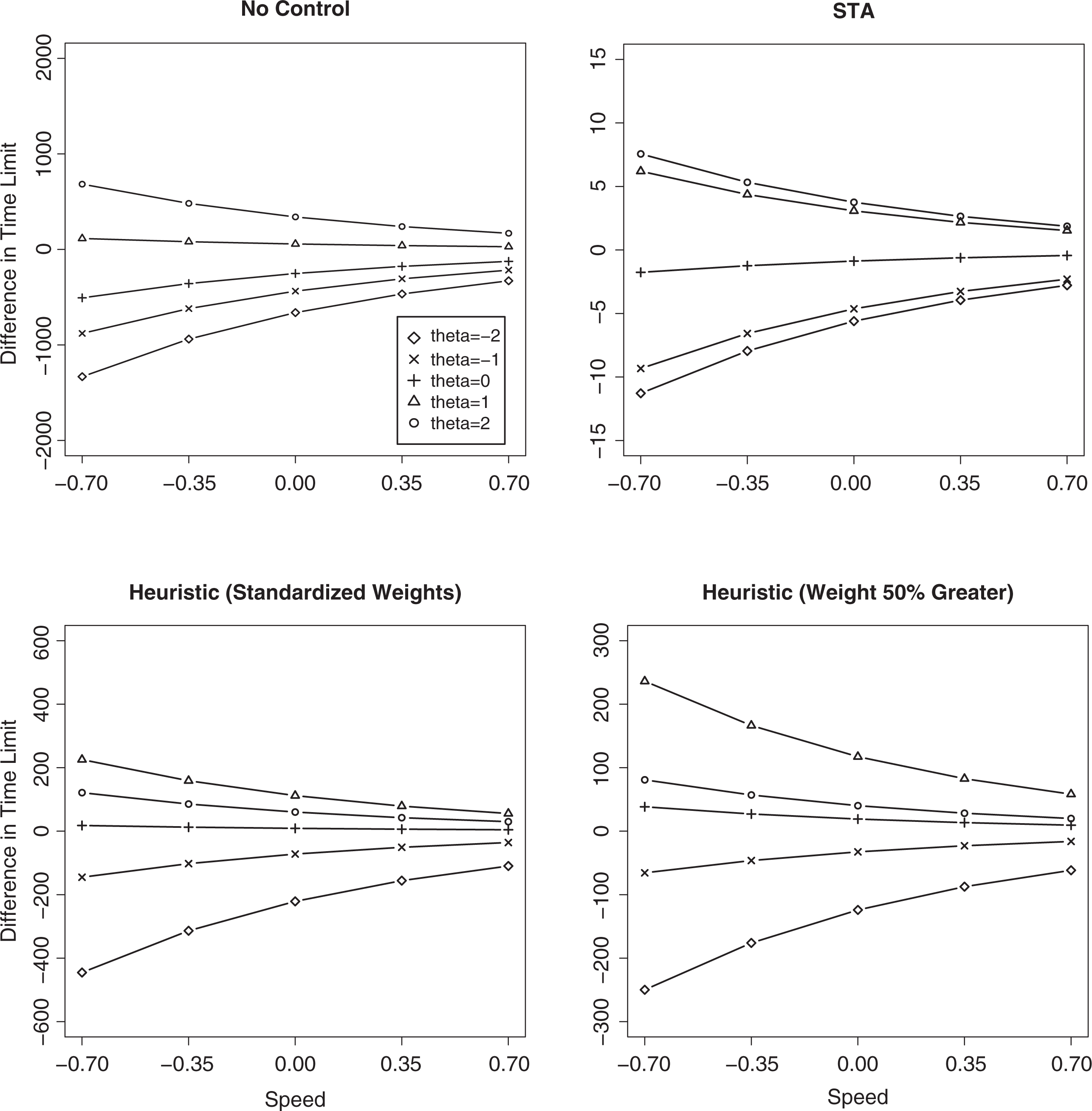
c. Average difference between the time limits for the reference and adaptive tests for the conditions with no control, STA, and two versions of the heuristic in seconds (π = .15).

As identical total-time distributions on the adaptive and reference test for each test taker implies identical risks of running out of time, we control the speededness during the adaptive test administrations in the strongest possible sense. For instance, for any given population of test takers, the method of control guarantees that the same number of test takers will experience exactly the same levels of time pressure on both tests. Observe that we are able to guarantee this without actually having to specify any explicit limit on the risk in Equation 1. We thus entirely avoid the problem of having to specify a minimally acceptable level of speed required to calculate such a limit.

Let $j = 1, . . ., n$ denote the items in the reference form. We use the item parameters in Equations 4 and 5 for the reference form to define target values

T_{q} \equiv \sum_{j = 1}^{n} q_{j},

and

T_{r} \equiv \sum_{j = 1}^{n} r_{j},

Each adaptive test is built to meet these two values. In order to achieve this goal, two different implementations of the idea are suggested. The first is a shadow-test method in which constraints based on the target values are inserted in the test-assembly model for each shadow test. A key advantage of this approach is that the constraints can be easily combined with whatever other constraints are required to meet the full set of content, statistical, and practical specifications for the test. The second method is a simple heuristic. It can be used for a plain adaptive test without any other constraints than the target values in Equations 11 and 12.

Implementations

Shadow-Test Approach (STA)

In STA, the selection of each item is preceded by the assembly of a shadow test from the item pool. Shadow tests are defined as fixed-form tests of the same length as the adaptive tests that (a) are maximal informative at the test takers current estimate of θ, (b) meet all constraints to be imposed on the test, and (c) contain all items already administered to the test taker (van der Linden, 2005, chap. 9). Basically, each next shadow test involves a reassembly of the remaining portion of the adaptive test, such that it still meets all constraints but now is maximally informative at the new θ estimate. The next item to be administered is the most informative item in the shadow test not yet seen by the test taker. All other free items are returned to the item pool. Because each next shadow tests meets all constraints and is maximally informative, the same automatically holds for the adaptive test.

In principle, shadow tests can be assembled using any method of constrained test assembly that is fast enough for use in real time. In the example later in this article, we used mixed integer programming (MIP) in combination with a fast commercial solver (IBM ILOG OPL version 6.3; International Business Machines Corporation, 2009) to identify the optimal shadow tests. For an application in R based on a free solver, see Diao and van der Linden (2011). The first step in this approach is the definition of 0-1 decision variables $x_{i}$ , $i = 1, . . ., I$ , for the items in the pool, which take the value $x_{i} = 1$ if item $i$ is selected for the new shadow test and $x_{i} = 0$ if it is not. These variables are used to model the objective function for the test as well as all necessary constraints implied by the test specifications. For a more comprehensive review of the possibilities of MIP modeling for automated test assembly, refer to van der Linden (2005).

Suppose the shadow test prior to the selection of the kth item in the adaptive test needs to be reassembled. Let $S_{k - 1}$ denote the indices of the $k - 1$ items already administered and $I_{i} ({\hat{θ}}_{k - 1})$ the value of the information function for item $i$ at the current estimate ${\hat{θ}}_{k - 1}$ . The core of the model for the reassembly of the shadow test is

\begin{matrix} m a x i m i z e \sum_{i = 1}^{I} I_{i} ({\hat{θ}}_{k - 1}) x_{i} & (m a x i m u m i n f o r m a t i o n a t {\hat{θ}}_{k - 1}), \end{matrix}

subject to

\begin{matrix} \sum_{i = 1}^{I} q_{i} x_{i} \leq T_{q} + δ_{q}, & (u p p e r l i m i t o n s u m o f q_{i}), \end{matrix}

\begin{matrix} \sum_{i = 1}^{I} q_{i} x_{i} \geq T_{q} - δ_{q}, & (l o w e r l i m i t o n s u m o f q_{i}), \end{matrix}

\begin{matrix} \sum_{i = 1}^{I} r_{i} x_{i} \leq T_{r} + δ_{r}, & (u p p e r l i m i t o n s u m o f r_{i}), \end{matrix}

\begin{matrix} \sum_{i = 1}^{I} r_{i} x_{i} \geq T_{r} - δ_{r}, & (l o w e r l i m i t o n s u m o f r_{i}), \end{matrix}

\begin{matrix} \sum_{i \in S_{k - 1}} x_{i} = k - 1, & (i t e m s a l r e a d y a d m i n i s t e r e d), \end{matrix}

\begin{matrix} x_{i} \in {0, 1}, i = 1, . . ., I . & (r a n g e o f v a r i a b l e s) . \end{matrix}

where ${\hat{θ}}_{k - 1}$ is the estimate of θ after the previous $k - 1$ items and $δ_{q}$ and $δ_{r}$ are tolerance parameters used to set small intervals about the target values $T_{q}$ and $T_{r}$ , respectively.

In a real-world application, the model may have to be extended with several other constraints, for instance, on the content distribution of the items in the test, to guarantee a desired answer-key distribution, prevent the administration of “enemy items,” constrain the range of readability indices, and so on. The solution to the model found by the solver is the string of 0s and 1s for the variables $x_{i},$ $i = 1, . . ., I$ , that identifies the items for the shadow test that meet all constraints and provide maximum information at ${\hat{θ}}_{k - 1}$ .

Heuristic

The heuristic we propose is analogous to a suggestion for automated test assembly by Luecht (1998). However, instead of the original application to a target for the test information function as the criterion for item selection, the current application is with respect to a combination of the targets $T_{q}$ and $T_{r}$ and the goal of maximum formation at $\hat{θ}$ .

The method consists of the calculation of the differences between the targets in Equations 11 and 12 and the sums of the parameters for the $k - 1$ items already administered to the test taker, division of the two differences in equal portions for the $n - k + 1$ remaining item slots in the adaptive test, and use of the result to select the kth item. More formally, we define

T_{q k} = (T_{q} - \sum_{i \in S_{k - 1}} q_{i}) / (n - k + 1),

and

T_{r k} = (T_{r} - \sum_{i \in S_{k - 1}} r_{i}) / (n - k + 1),

as the target values for the selection of the kth item. The kth item is selected to have both maximum information at ${\hat{θ}}_{k - 1}$ and $q_{i}$ and $r_{i}$ parameters as close as possible to $T_{q k}$ and $T_{r k}$ , respectively. The three objectives are combined in the following criterion for item selection:

i_{k} = arg max_{j} {I_{i} ({\hat{θ}}_{k - 1}) - w_{q} |q_{i} - T_{q k}| - w_{r} |r_{i} - T_{r k}|; j \in R_{k}},

where $R_{k} = {1, . . ., I} ∖ S_{k - 1}$ is the set of indices of the remaining items in the pool after $k - 1$ items have been administered. Observe that the algorithm is “forward looking” in that it uses the current gap between the actual sums of the $q_{i}$ and $r_{i}$ parameters and the targets in Equations 11 and 12 to set a criterion for the next item. In doing so, it prevents from a scenario in which all best items are immediately selected, leaving us with the lesser items to finalize the test. In addition, if we are occasionally forced to select an item with a contribution too low or high relative to Equations 20 and 21, the recalculation of these values at the next step automatically compensates for the fact.

The weights $w_{q}$ and $w_{r}$ in Equation 22 can be used to prioritize the individual objectives. This should be done after a correction for the scale differences between them. In the simulation studies below, we used the average values of $I_{i} ({\hat{θ}}_{k - 1})$ and the $q_{i}$ and $r_{i}$ parameters for the remaining set of items $R_{k}$ in the pool to correct for scale differences and opted for equal priorities for all three objectives. As the numbers of items cancel, the choice amounts to

w_{q k} = \frac{\sum_{i \in R_{k}} I_{i} ({\hat{θ}}_{k - 1})}{\sum_{i \in R_{k}} q_{i}},

and

w_{r k} = \frac{\sum_{i \in R_{k}} I_{i} ({\hat{θ}}_{k - 1})}{\sum_{i \in R_{k}} r_{i}} .

Evaluation Study

Simulation studies were conducted to evaluate the effectiveness of the STA and heuristic in eliminating differences in speededness between test takers under a variety of conditions. More particularly, we looked at the extent to which the two methods approximated the desired degree of speededness for the adaptive test for test takers with different abilities operating at different speeds. In addition, we assessed the possible price to be paid for the control of the speededness in the form of loss of precision of ability estimation due to the extra constraints or objectives enforced on the item selection.

Data

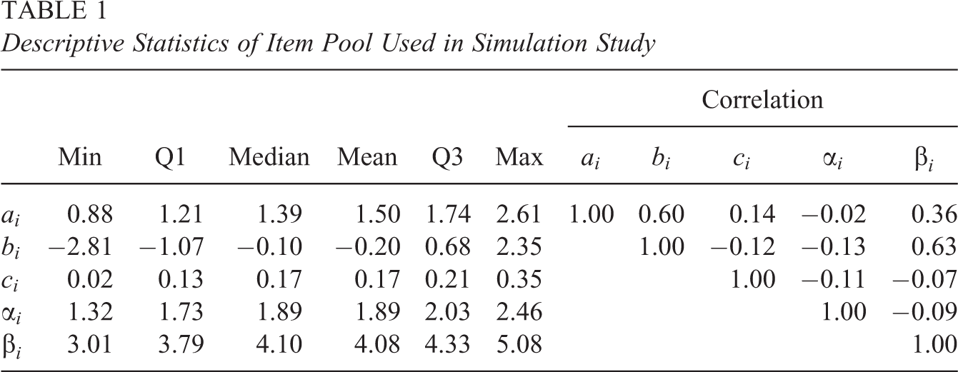
Adaptive test administrations were simulated from a pool consisting of a set of 185 items sampled from a retired pool from a large-scale testing program. The $α_{i}$ for $β_{i}$ parameters for items in the original pool were estimated from a data set with the RTs for more than 10,000 test takers, using a Bayesian method with Gibbs sampling from the posterior distributions of the parameters (for a description of the method, see van der Linden, 2006). We only selected items that showed satisfactory fit to the model. The ranges of the estimates were [1.32,2.46] for the $α_{i}$ and [3.01,5.08] for the $β_{i}$ parameters. The mean estimate of the speed parameters τ for the test takers in the data set was centered on $μ_{\hat{τ}} = 0.$ The estimates had an empirical standard deviation of approximately $σ_{\hat{τ}} = .35$ . The estimated parameter values were used as the true values in the simulation study. The same holds for the item parameters in the three-parameter logistic (3PL) response model; the true values used for these parameters were the estimates that had been used operationally in the testing program. Table 1 gives some descriptive statistics of the item parameter distribution in the item pool. For later reference, observe the positive correlation between the $a_{i}$ and $b_{i}$ parameters and the $b_{i}$ and $β_{i}$ parameters. The former implies an item pool that is generally less informative at the lower end of the scale. The latter is a potential source of differential speededness; without any control, it would have the item-selection algorithm select the more time-intensive items for the more able test takers.

Table 1

Descriptive Statistics of Item Pool Used in Simulation Study

	Min	Q1	Median	Mean	Q3	Max	Correlation
	Min	Q1	Median	Mean	Q3	Max	$a_{i}$	$b_{i}$	$c_{i}$	$α_{i}$	$β_{i}$
$a_{i}$	0.88	1.21	1.39	1.50	1.74	2.61	1.00	0.60	0.14	−0.02	0.36
$b_{i}$	−2.81	−1.07	−0.10	−0.20	0.68	2.35		1.00	−0.12	−0.13	0.63
$c_{i}$	0.02	0.13	0.17	0.17	0.21	0.35			1.00	−0.11	−0.07
$α_{i}$	1.32	1.73	1.89	1.89	2.03	2.46				1.00	−0.09
$β_{i}$	3.01	3.79	4.10	4.08	4.33	5.08					1.00

Adaptive tests with a fixed length of 20 items for test takers with a true ability parameter equal to $θ = - 2, - 1, 0, 1,$ or $2$ were simulated $.$ For each θ, we replicated 500 simulations. Item selection was according to the maximum-information criterion. For ability estimation, we used expected a posteriori (EAP) estimation with a uniform prior over [ $- 4, 4$ ]. The first item was chosen to be optimal at ${\hat{θ}}_{_{0}} = 0$ .

Four different conditions were simulated:

No control of speededness;

Control of speededness using the STA in Equations 13 –19;

Control of speededness using the item-selection heuristic in Equation 22 with the standardized weights in Equations 23 and 24.

Control of speededness as in Condition 3, but now with weights that were 50% greater than the standardized weights in Equations 23 and 24.

The fourth condition was included to explore the effects of relatively greater weights for the last two objectives in Equation 22. In principle, increasing these weights means better control of speededness, but possibly at the price of a less informative adaptive test. The STA was implemented using tolerances

δ_{q}

and

δ_{r}

in Equations 14 to 17 set equal to 0.5% of the target values.

The reference test consisted of 20 items randomly sampled from the pool. The target values for the reference test in Equations 11 and 12 were $T_{q} = 1, 601$ and $T_{r} = 49, 592$ . Figure 1 shows the total-time distributions in Equations 8 –10 for this single reference test for test takers working at speed $τ = - .70,$ $.35,$ $0,$ $.35$ , and $.70$ . The speed levels were chosen to cover the approximate range of $μ_{\hat{τ}} \pm 2 σ_{\hat{τ}}$ for the test takers in the original data set. Clearly, variation of the speed parameter is consequential. The two most extreme distributions, which were four standard deviations apart ( $τ = - .70$ and $τ = .70$ ), had locations at approximately 800 and 3,200 s.

For each of the five τ levels, we calculated the time limit $t_{l i m}$ required for the reference test to realize the risk levels of $π = .05$ , $.10$ , and $.15$ using

t_{l i m} = F_{T_{t o t}}^{- 1} (1 - π | τ, α, β),

which is the value of the quantile function for the total-time distribution (inverse of the distribution function in Equation 1) at $1 - π$ . The range of risk levels was chosen to represent a testing program with an intentionally low degree of speededness. The results in Table 2 show time limits that varied widely across the chosen combinations of speed and risk. The limit required for the slowest speed in combination with the lowest risk level was approximately 4 times higher than the one for the highest speed in combination with the highest risk level ( $t_{l i m} = 66^{'} 51^{''}$ vs. $15^{'} 09^{''}$ ).

Table 2

Time Limits (in minutes) on the Reference Test Required to Realize Risk Levels $π = .05, .10$ , or $.15$ for a speed of $τ = - .70, - .35, 0, .35,$ or $.70$

Risk ( $τ$ )	Speed ( $τ$ )
Risk ( $τ$ )	−.70	−.35	0	.35	.70
.05	$66^{'} 51^{''}$	$47^{'} 06^{''}$	$33^{'} 12^{''}$	$23^{'} 23^{''}$	$16^{'} 29^{''}$
.10	$63^{'} 34^{''}$	$44^{'} 48^{''}$	$31^{'} 34^{''}$	$22^{'} 35^{''}$	$15^{'} 41^{''}$
.15	$61^{'} 27^{''}$	$43^{'} 18^{''}$	$30^{'} 35^{''}$	$21^{'} 31^{''}$	$15^{'} 09^{''}$

As the methods of control of differential speededness did not assume estimation of any speed parameter during testing, it was not necessary to manipulate this parameter in our study. The only thing we had to do to evaluate the two methods was to record the $α_{i}$ and $β_{i}$ parameters in the RT model for the items administered to the test takers. The actual level of speededness was evaluated afterward, comparing the time limits for the reference test in Table 2 with the time limits that would have been required for the actual items in the adaptive tests to create the same risk at the same levels of speed. This choice of evaluation criterion allowed us to evaluate speededness in a directly interpretable metric, namely as a difference between actual and required testing time.

The estimation errors ${\hat{θ}}_{k} - θ$ recorded during the simulation of the adaptive tests were used to calculate the bias and MSE functions for the final ability estimates as

E [({\hat{θ}}_{k} - θ) |θ],

and

E [({\hat{θ}}_{k} - θ)^{2} |θ] .

Results

Figure 2 shows the average difference between the actual and required time limits in seconds as a function of the τ values for a risk of $π = .05$ (panel a), $π = .10$ (panel b), and $π = .15$ (panel c) for the four conditions. The large differences for the condition of no control show the seriousness of the problem of differential speededness in adaptive testing. The problem was especially dramatic for test takers with high ability who worked slowly; on average, they would have needed at least 15 more minutes to finish in time. On the other hand, low-ability test takers at the same level of speed had an average of approximately 25 min left when they finished the test. This differential effect is entirely due to the combination of the already observed positive correlation between the difficulties and time intensities of the items ( $r = .63$ ) and the adaptive algorithm selecting items with difficulties matching the test takers’ abilities. The same combination explains the general order of the curves for the θ levels in each of the plots in Figure 2.

The shadow-test method did a superior job controlling the speededness of the adaptive test. No matter the level of risk, speed, or ability, the presence of the constraints in Equations 14 to 17 guaranteed a maximum absolute difference between the time limit for the reference test and the limits required for the adaptive test smaller than 10 seconds. The two versions of the heuristic method had more difficulty controlling the degree of differential speededness, but all plots show results that tend to be much closer to those for the shadow-test method than for the condition without control. Generally, as expected, the results for the higher weights were somewhat better, especially for the low ability group.

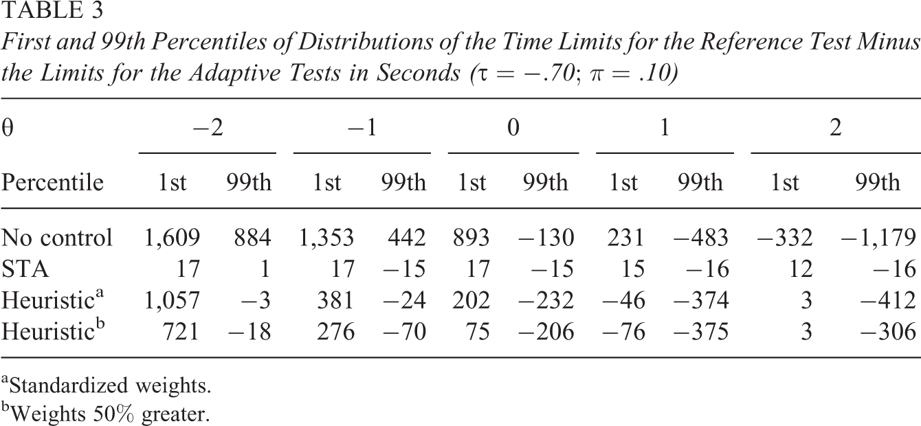
In principle, small differences between average levels of speededness do not imply anything at the level of the individual test takers. The standard deviations of the time limits required by the adaptive tests in Figure 3, however, confirm the differences in control between the four conditions. The variation between the limits for the condition without any control was huge, whereas the shadow-test method showed negligible variation (all standard deviations smaller than 10 seconds). Again, the results for the heuristic were closer to those for the shadow-test method than for the condition without any control. For all ability groups, the two versions of the heuristic yielded approximately equal standard deviations, with the exception of some improvement for the low-ability group for the version with the higher weights. Thus, the better results for the average differences in time limit by the latter were accompanied by a somewhat smaller variability across the test takers. The same general pattern of results for the four methods is shown by the 1st and 99th percentiles of their distributions of the time limit for the reference test minus the limits for the adaptive tests in Table 3. Note that the case for $τ = - .70$ in this table is the one with the largest standard deviations in Figure 3. The results for $π = .05, .10,$ and $.15$ were entirely comparable.

Table 3

First and 99th Percentiles of Distributions of the Time Limits for the Reference Test Minus the Limits for the Adaptive Tests in Seconds ( $τ = - .70;$ $π = .10$ )

θ	−2		−1		0		1		2
Percentile	1st	99th	1st	99th	1st	99th	1st	99th	1st	99th
No control	1,609	884	1,353	442	893	−130	231	−483	−332	−1,179
STA	17	1	17	−15	17	−15	15	−16	12	−16
Heuristic^a	1,057	−3	381	−24	202	−232	−46	−374	3	−412
Heuristic^b	721	−18	276	−70	75	−206	−76	−375	3	−306

^aStandardized weights. ^bWeights 50% greater.

Figure 3.

a. Standard deviation of the required time limits for the adaptive test for the conditions with no control, shadow-test approach (STA), and two versions of the heuristic (π = .05).

Figure 3.

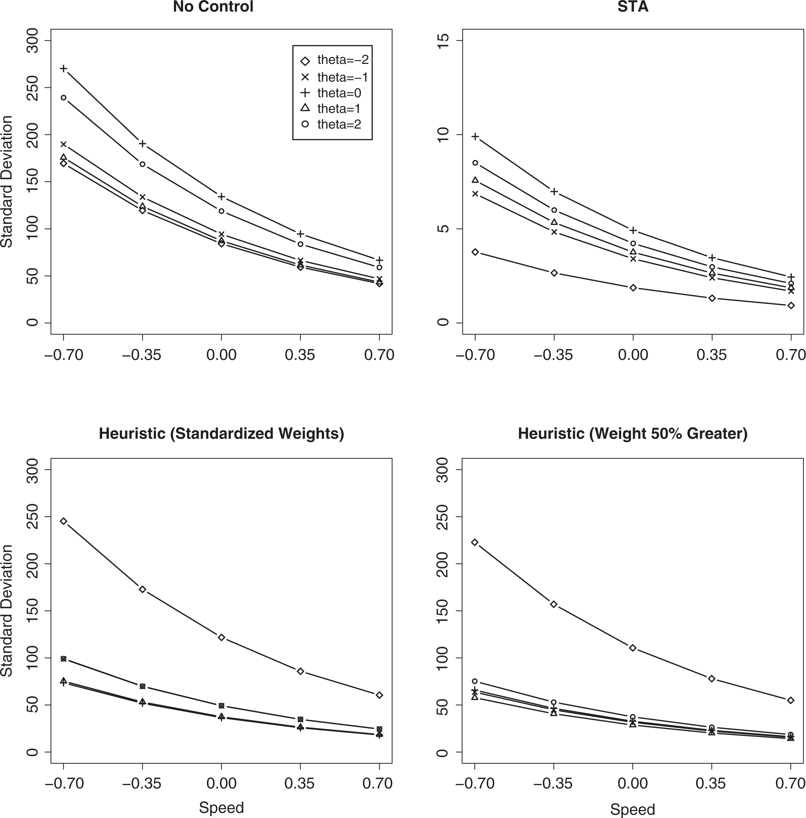
b. Standard deviation of the required time limits for the adaptive test for the conditions with not control, STA, and two versions of the heuristic (π = .10).

Figure 3.

c. Standard deviation of the required time limits for the adaptive test for the conditions with no control, STA, and two versions of the heuristic (π = .15).

Generally, the control of speededness resulted in negligible loss of statistical quality of the ability estimates. The plots in Figure 4 show the estimated bias and MSE functions for the two control methods that are essentially the same as for adaptive testing without any control. The only differences are a positive bias for the shadow-test method and a somewhat larger MSE for the two versions of the heuristic method at $θ = - 2$ . As the precision of estimation at all other $θ$ values was virtually identical, we expect these incidental exceptions to be due to less information in the items at the lower end of the scale (role of the guessing parameter and positive correlation between the $a_{i}$ and $b_{i}$ parameters, $r = .60$ ).

Figure 4.

Estimated bias and MSE as a function of θ for the conditions with no control, shadow-test approach (STA), and two versions of the heuristic.

Concluding Remarks

The empirical study showed how serious the effects of differences in item selection on the testing time can be if we do not control for differential speededness in adaptive testing. It also showed that the effects can be effectively removed by imposing two simple constraints on the RT parameters of the items during item selection.

Another novelty of the method is the absence of any estimation of the test taker’s actual speed during the test. Besides, it does not require any projection of the time needed by the test taker for the remaining portion of the test. And the idea of matching the time characteristics of the adaptive tests with a reference test of proven quality is also practically convenient: It prevents the setting of a minimally acceptable level of speed for the test takers required for direct control of the risk in Equation 1. In spite of control of differential speededness up to a few seconds by the STA method, there appears to be hardly any price in the form of deteriorated ability estimation.

It is possible to compare the results for the current STA method with those for the earlier method in van der Linden (2009a). Both studies had an item pool for the adaptive test sampled from the same inventory of items and an identical setup of the simulated adaptive tests. The only differences existed in a much smaller item pool for the current study (185 vs. 350 items) in combination with a longer test (20 vs. 15 items). The former favors the earlier study; the latter our current study. The relevant comparison is between the average differences between the actual and required time limits in our current study (Figures 2 and 3) and the average time spent on the adaptive test in the earlier study (van der Linden, 2009a, figure 1; this figure also shows the time limits that were simulated). While the current study demonstrated control up to differences smaller than 10 s for each of the ability groups working at any of the levels of speed, the earlier study yielded much greater variation. In fact, only the differences for the test takers with ability $θ = 2$ working at the slowest simulated speed in the earlier study came close to our current results; for all other conditions, much larger differences were obtained (running up to some 1,700–1,800 seconds for the group with $θ = - 2$ working at the highest simulated speed). The explanation is the one-sided nature of the earlier method. As already indicated, it was designed only to guarantee completion of the test within the available time, which it did remarkably well. In spite of the much more homogenous, two-sided control by the new method, a comparison between the bias and MSE plots in Figure 4 with those in the earlier study (van der Linden, 2009, figures 5–6) show results with exactly the same pattern: hardly any bias or MSE for the simulated ability levels $θ = - 1,$ $0,$ and $1$ and similar bias and MSE at $θ = - 2$ and $2$ .

Finally, observe again that the two constraints are only on two different sums of item parameters. It is thus not necessary to match these parameters with the ones for the reference test on an item-by-item basis. The leeway generated by this relaxation explains why there was no significant loss of statistical precision in the ability estimates for the two methods of speededness control.

Footnotes

Declaration of Conflicting Interests

The authors declared no potential conflicts of interest with respect to the research, authorship, and/or publication of this article.

Funding

The authors received no financial support for the research, authorship, and/or publication of this article.

References

Bridgeman

Cline

(2004). Effects of differentially time-consuming tests on computerized-adaptive test scores. Journal of Educational Measurement, 41, 137–148.

Diao

van der Linden

W. J.

(2011). Automated test assembly using lp_solve version 5.5 in R. Applied Psychological Measurement, 35, 398–409.

Fenton

(1960). The sum of log-normal probability distributions in scatter transmission systems. IRE Transactions on Communication Systems, 8, 57–67.

Finger

Chuah

S. C.

(2009, April). Response-time model estimation via confirmatory factor analysis. Paper presented at the annual meeting of the National Council on Measurement in Education, San Diego, CA.

International Business Machines Corporation. (2009). IBM ILOG OPL, Version 6.3 [Software program and manual]. Armonk, NY: Author.

Klein Entink

R. H.

Fox

J.-P.

van der Linden

W. J.

(2009). A multivariate multilevel approach to simultaneous modeling of accuracy and speed on test items. Psychometrika, 74, 21–48.

Luecht

R. M.

(1998). Computer-assisted test assembly using optimization heuristics. Applied Psychological Measurement, 22, 224–236.

van der Linden

W. J.

(2005). Linear models for optimal test assembly. New York, NY: Springer.

van der Linden

W. J.

(2006). A lognormal model for response times on test items. Journal of Educational and Behavioral Statistics, 31, 181–204.

10.

van der Linden

W. J.

(2007). A hierarchical framework for modeling speed and accuracy on test items. Psychometrika, 72, 287–308.

11.

van der Linden

W. J.

(2009a). Predictive control of speededness in adaptive testing. Applied Psychological Measurement, 33, 25–41.

12.

van der Linden

W. J.

(2009b). Conceptual issues in response-time modeling. Journal of Educational Measurement, 46, 247–272.

13.

van der Linden

W. J.

(2011a). Setting time limits on tests. Applied Psychological Measurement, 35, 183–199.

14.

van der Linden

W. J.

(2011b). Test design and speededness. Journal of Educational Measurement, 48, 44–60.