Screening Test Items for Differential Item Functioning

1. Introduction

Differential item functioning (DIF) is an important consideration in the construction of standardized educational tests. It is defined for a partition of the examinees into two groups, such as men and women or majority and minority, referred to as the reference and focal groups. A test item is said to function differentially (to have high DIF) for these two groups if there are substantial differences in the within-group distributions of the scores on the item even after conditioning on the overall test score. For a dichotomous item, an established method (Holland & Thayer, 1988) quantifies DIF by the conditional log odds ratio of the correct response, given the overall score. This ratio is assumed to be constant across the values of the overall score. High DIF corresponds to a large absolute value of the common log odds ratio. Items with high DIF are undesirable in an operational test and procedures for screening them out, reviewing their wording and presentation, or excluding them have been applied in test construction since several decades ago (Osterlind & Everson, 2009). Studies of the causes of DIF and its dependence on the item’s content and context in the test (e.g., its order in the test or in a block) also have a long history (Holland & Wainer, 1993).

We introduce a method for screening test items for high DIF in which every item is classified as suitable or unsuitable by the criterion of minimizing the expectation of a specified loss function. Two key parameters have to be specified by the analyst: one that characterizes what amounts to high DIF and another that quantifies the losses due to the two kinds of incorrect classification. A similar approach was developed by Zwick, Thayer, and Lewis (2000). They proposed a single criterion on which to classify the items (Equation 8 in Zwick, Thayer, & Lewis, 2000), although Zwick, Ye, and Isham (2012) used a generalization. We consider a range of criteria that correspond to different levels of aversion to retaining an item with high DIF in the test. We address the issue of uncertainty about this level of aversion by an approach that can be regarded as a sensitivity analysis.

The discussion of Zwick et al. (2000) and the internal memoranda they cite (Holland, 1987a, 1987b) raise the concern that a hypothesis test regards the null hypothesis of no DIF as the default. If the DIF of an item is estimated with large sampling variation, then the item is likely to be classified as not having substantial DIF, because the power of the related test is low. In our perspective, the burden of evidence about the good properties of a test item is on the test developer, and therefore an item with poorly estimated DIF should be classified as unsuitable. More precisely, an item should be classified as suitable only when there is ample evidence that its DIF is not excessive.

Sinharay, Dorans, Grant, and Blew (2009) and Zwick et al. (2012) propose methods for incorporating external information in DIF estimation by (empirical) Bayes methods. Our approach, an application of decision theory, has a Bayesian variant, which requires prior distribution of the item parameters as an additional input. In fact, decision theory is more naturally formulated in the Bayesian paradigm; see Berger (1985), Lindley (1985), and DeGroot (2004) for background.

We present an application to the scaled logarithm of the Mantel–Haenszel (MH) common odds ratio estimator (Holland & Thayer, 1988), also referred to as the MH Delta DIF (D-DIF) statistic. The scaling amounts to multiplying the common log odds ratio and its estimator by −2.35. The only properties of this estimator we assume are (approximate) normality, absence of bias, and knowledge of its sampling variance. The method requires only slight changes for other estimators of item-level DIF that have these properties. The scaling of the MH D-DIF statistic makes the value of δ = 1.0 a reasonable (and in some contexts well established) borderline between acceptable and excessive level of DIF. Some complications arise for methods of DIF analysis for which such a borderline value is not established. In an implementation of our method it suffices to specify a range of plausible values of δ.

We interpret a procedure for the inspection of DIF of the items of a test as screening, assuming that each item has to be unambiguously assigned to one of the two categories: suitable (with negligible DIF) or unsuitable (with high DIF). In practice, “negligible DIF” is interpreted as small or acceptable DIF, because the absence of DIF is in most contexts an unattainable ideal (Longford, 1995, chap. 5; Longford, Holland, & Thayer, 1993). Screening for a condition in medical practice, in which each subject is assessed as being either negative (condition absent) or positive (condition present), has obvious parallels with inspecting test items for DIF. In both settings, each inspected unit (a person/patient or a test item) is associated with the value of a variable called the marker, denoted by Δ. The value of Δ is measured or estimated subject to error, by Δ ˆ , with an estimated or known (measurement or sampling) variance s ². The classification of each unit is based on its values of Δ ˆ and s.

Denote the marker for a test item by Δ M H and suppose its values in the range H = ( − δ , δ ) are acceptable. We would like to classify the item as either belonging to H or not. The value of the marker is recorded subject to estimation error by an unbiased estimator Δ ˆ M H . We assume that it is the MH D-DIF statistic derived from the results of Mantel and Haenszel (1959). Its standard error, denoted by s, is estimated by the method of Phillips and Holland (1987). In common with other methods, we ignore the uncertainty in the estimation of s or s ². The test constructors’ intent is to ensure that no unsuitable items are present in the final version of the test. Suppose their perspective is well described by the following two statements. If a suitable item, one with Δ M H ∈ H , is excluded from the pool of items from which the test is to be assembled, we incur one unit of loss (harm, damage, erosion of quality, or the like). If an item with Δ M H ∉ H is included in the pool, the harm amounts to R units. We refer to R as the penalty ratio. No loss is incurred if the item is classified correctly. More realistic perspectives, which require more extensive evaluations, are introduced in Section 4.

Setting the values of δ and R may be contentious, but this problem can be alleviated by declaring plausible ranges of δ and R, ( δ L , δ U ) and ( R L , R U ) , respectively. In most settings, informed experts would readily agree that R L > 1 and maybe also that δ U ≤ 1 . The procedure proposed in Section 2 is applied for the four pairs ( δ L , R L ) , ( δ L , R U ) , ( δ U , R L ) , and ( δ U , R U ) . If the same category is concluded for an item in all four cases, then this category is adopted. Only two analyses have to be conducted when there is no uncertainty about δ, when δ = δ L = δ U . If the item is classified equivocally, as suitable for one but unsuitable for another of the four pairs ( δ , R ) , then we reach an impasse because it is plausible that the expected loss is smaller for either category. An intermediate category could be defined for such items and they could be subjected to a review procedure less stringent than items classified unequivocally as unsuitable. If impasse occurs for more than only one or two items, and the experts are available for another consultation, then the plausible ranges of δ and R could be reviewed and reduced. However, all the parties involved should be satisfied that all values outside these ranges can be ruled out—that they are implausible.

The method described in the next section is an elementary application of decision theory; for an application to medical screening that is adapted here to DIF, see Longford (2013a), and for theoretical background and other examples, see Longford (2013b). Section 3 gives an illustrative example and Section 4 presents some refinements in which the loss depends on the value of Δ M H . A simulation study based on an operational administration of a test of English language proficiency used worldwide is described in Section 5. The article is concluded by a discussion.

2. Classifying an Item

Suppose the statistic Δ ˆ M H for a test item has normal distribution with expectation Δ M H and standard error s; Δ ˆ M H = Δ M H + s X , where X has the standard normal distribution. After establishing the value of Δ ˆ M H , its status is changed from a random variable to a constant. Now we regard Δ M H = Δ ˆ M H − s X as a random variable. Owing to symmetry of the normal distribution, it is also normally distributed. This change of status from a fixed to a random quantity and vice versa is common in the Bayesian paradigm, but all the other elements of the method introduced in this section are entirely frequentist. A Bayesian adaptation is discussed in Section 5.

Denote by φ the density and by Φ the distribution function of the standard normal distribution. If we classify the item as unsuitable, then the expectation of the loss we incur is equal to the integral of the (one unit) loss multiplied by the density of Δ M H over the range H that corresponds to suitable items. This integral is equal to the probability that the item is suitable:

L A = P Δ M H ∈ H | Δ ˆ M H ; s = 1 s ∫ − δ δ ϕ x − Δ ˆ M H s d x = Φ δ − Δ ˆ M H s − Φ − δ − Δ ˆ M H s = Φ z + − Φ z − ,

1

where z + = ( Δ ˆ M H + δ ) / s and z − = ( Δ ˆ M H − δ ) / s . If we classify the item as suitable, then the expected loss is L H = R P ( Δ M H ∉ H | Δ ˆ M H ; s ) = R ( 1 − L A ) . We define the balance as the difference Δ L = L A − L H . It is equal to ( R + 1 ) L A − R . When the balance Δ L is negative, classifying the item as unsuitable results in smaller expected loss. When Δ L > 0 , classifying the item as suitable is preferred. This rule is equivalent to classifying the item as unsuitable when

L A < R R + 1 .

2

For given values of δ and s, L A is an increasing function for Δ ˆ M H < 0 and decreasing for Δ ˆ M H > 0 . It attains its maximum of 2 Φ ( δ / s ) − 1 at Δ ˆ M H = 0 . Therefore, an item with a given standard error s would be classified as unsuitable irrespective of the value of Δ ˆ M H when the inequality in Equation 2 holds even for Δ ˆ M H = 0 . This condition is equivalent to 2 Φ ( δ / s ) − 1 < R / ( R + 1 ) , and the solution of this inequality is

δ < s Φ − 1 2 R + 1 2 R + 2 .

3

Situations in which this inequality is satisfied can be interpreted as follows:

However, they are unlikely to arise in any practical setting with reasonable values δ and R and nontrivial (effective) sample size to which s is related. The values of Δ ˆ M H for which L A = R / ( R + 1 ) are called borderline. For given s, δ, and R, they can be found by the Newton–Raphson algorithm. The algorithm is described in Appendix A.

The rule given by Equation 2 is related to the rule for rejecting the hypothesis that | Δ M H | < δ with test size α = 1 / ( R + 1 ) , after replacing the simple hypothesis H 0 : Δ M H = 0 with the composite hypothesis H δ : Δ M H ∈ ( − δ , δ ) . In both cases, the probability of an error of one kind (flagging a suitable item or Type I error) is 1 / ( R + 1 ) . This probability has a different meaning in the two approaches and is evaluated differently. In hypothesis testing, the rate of Type I error is controlled for Δ M H = ± δ , whereas our counterpart given by Equation 1 entails integration over the range ( − δ , δ ) . The conventional test size of α = 0.05 corresponds to R = 19. While objections to this value of α are rarely constructive, the definition of the penalty ratio R opens up an avenue toward a calibration of the procedures for DIF that balances the effort of item preparation, the need for an even representation of the cognitive domain in the test, and similar specification constraints with the quality of the test that is associated with the DIF of its items contained within the range ( − δ , δ ) . The setting of δ is also a nontrivial matter but, related to the scale on which DIF is estimated, its value provides an unambiguous indication of what level of DIF is tolerated. Zwick et al. (2000) and Holland (2004) regard δ = 1 as appropriate for the (scaled) MH D-DIF statistic. We use this standard in Sections 3 and 5.

The value of the expected loss, min ( L H , L A ) , added up (or averaged) over the items in the test, can be adopted as a test-level measure of the uncertainty about the presence of unacceptable DIF in the test. Its purpose need not be another review of the test, but it may be to monitor whether the markers Δ M H are estimated with sufficient precision. At an extreme, the classification would be almost perfect with small standard errors s, but the sample sizes required for pretesting that would yield them may be unattainable. In contrast, the quality of screening would obviously suffer if many values of s were too large, and the total of the expected losses would reflect this.

The key property of a loss function is additivity, meaning that it can be treated like a (monetary) currency. That is, the loss of a units in one instance and of b in another is for all purposes equivalent to the loss of a + b units. Without this condition, the expectations of the loss and their totals over the items are not meaningful. If we are satisfied that the loss associated with misclassifying a suitable item is constant, then no generality is lost by setting this constant to unity because multiplying the loss function by a positive constant does not alter the problem. It corresponds to the conversion to a different currency for the loss. However, a nonlinear (monotone) transformation of Δ M H has to be accompanied by a matching transformation of the loss function.

3. Example

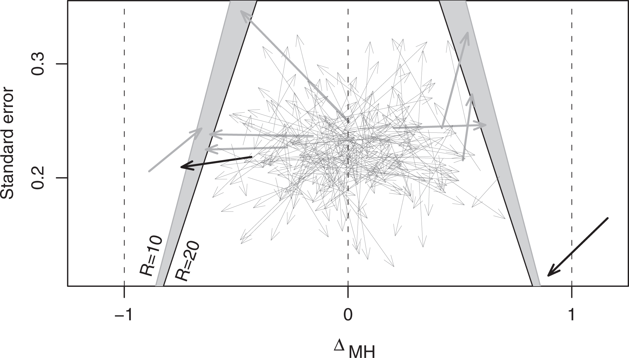
For illustration, we generated the values of Δ M H , s, Δ ˆ M H , and s ˆ for a set of 250 items by the following random process, fine-tuned by trial and error. The values of Δ M H are a random sample from a scaled t distribution with 5.5 degrees of freedom and the squared standard errors s ² of Δ ˆ M H an independent random sample from the uniform distribution on (0.040, 0.0625). The estimates Δ ˆ M H are generated as draws from the normal distribution with mean Δ M H and variance s ², and the estimates s ˆ 2 as draws from scaled χ² distributions, with degrees of freedom themselves drawn from the uniform distribution on (15, 25). All the draws are mutually independent. In both instances, scaling refers to multiplication by a positive constant.

The generated data set is plotted in Figure 1. Each item is represented by an arrow aiming from ( Δ M H , s ) to ( Δ ˆ M H , s ˆ ) . In a practical setting, only the values at the tips of the arrows would be available. The items represented by the arrows drawn by thicker lines are classified as unsuitable with the settings δ = 1 and R = 10 or 20. The arrows for the two items that are classified as unsuitable for both R = 10 and 20 are drawn by thick black lines. Seven other items are classified as suitable for R = 10 but not for R = 20 ; the corresponding arrows are drawn by thick gray lines.

OPEN IN VIEWER

Figure 1.

The values of Δ M H , Δ ˆ M H , s, and s ˆ for a set of 250 items and their classification for δ = 1 and R = 10 and 20. The arrows aim from the quantities ( Δ M H , s ) to their estimates ( Δ ˆ M H , s ˆ ) . A computer generated example.

In this example, 1 item has value of Δ M H outside the range (−1, 1). Its estimate Δ ˆ M H is within the range, and yet it is classified as unsuitable. Given the aversion to including an unsuitable item, as qualified by the value of R, caution is exercised and an item is classified as unsuitable if its value of Δ M H could plausibly be outside (−δ, δ). One of the misclassified items has Δ M H very close to zero, but its estimation error happens to be extreme, and its standard error is also overestimated (the long arrow heading northwest). The misclassifications highlighted in Figure 1 are errors that one would like to avoid, but they are more appropriately described as the price for uncertainty about the values of Δ M H .

The two shaded wedges symmetrically located around the vertical zero are delimited by the borderline functions for R = 10 (gray, further away from zero) and R = 20 (black, closer to zero). The wedges represent the “gray area” in which items are classified equivocally. The borderline functions have very little curvature within the plotted range. Their values for s = 0 are ±δ. They converge to zero as s → + ∞ when R > 1 and diverge to ± ∞ when R < 1 . An item with poorly estimated Δ M H , with very large s, is classified to the category for which the consequences of an error are less serious: as unsuitable when R > 1 and as suitable when R < 1 . Established procedures based on hypothesis testing are likely to classify an item with large s as suitable because the relevant test has low power, ignoring the consensus that R > 1 .

The totals of the expected losses are 13.14 and 22.39 for R = 10 and 20, respectively. If the exact standard errors were known, 4 items would be misclassified with R = 10 and further 2 also with R = 20 . The totals of the expected losses would be 11.49 (R = 10) and 19.87 (R = 20). If all the standard errors and their estimates were reduced by 10%, all items would be classified correctly with R = 10 and only 3 items would be misclassified with R = 20; the totals of the expected losses would be 8.43 and 14.76, respectively.

The number of highlighted items in Figure 1 is not a good estimator of the number of unsuitable items in the pool. A more appropriate estimator is given by the total of the probabilities

P ( | Δ M H | > δ ) = 1 − L A .

Assuming independence, the corresponding sampling variance is the total of the elementary variances L A ( 1 − L A ) . For δ = 1 , we obtain the estimate 1.43 (items) with standard error 1.16. The probabilities L A = Φ ( z + ) − Φ ( z − ) ignore the uncertainty about the standard error of Δ ˆ M H . This can be taken care of by evaluating each L A as ψ k ( z + ) − ψ k ( z − ) , where ψ k is the distribution function of the t distribution with k degrees of freedom. The standard evaluation corresponds to k → + ∞ . The number of degrees of freedom is not known, but intuition suggests that it is not very large. For k = 25, we obtain the estimate of the number of unsuitable items 1.83 with standard error 1.32; for k = 15, these values are 2.16 and 1.43.

4. Some Refinements

The loss caused by failing to flag a high-DIF item can be set to depend on Δ M H itself, as suggested by Zwick et al. (2000). This perspective is catered for by the piecewise linear loss, defined as R 0 + R 1 ( Δ M H − δ ) for an item with Δ M H > δ and as R 0 + R 1 ( − Δ M H − δ ) for an item with Δ M H < − δ , when it is incorrectly classified as suitable; R 0 and R 1 are positive constants. The loss for misclassifying a suitable item is equal to unity.

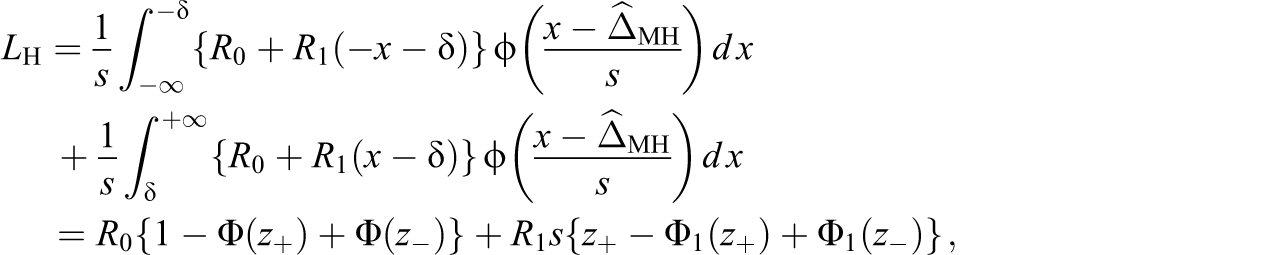
The expected loss for incorrect flagging is

L H = 1 s ∫ − ∞ − δ { R 0 + R 1 ( − x − δ ) } ϕ x − Δ ˆ M H s d x + 1 s ∫ δ + ∞ { R 0 + R 1 ( x − δ ) } ϕ x − Δ ˆ M H s d x = R 0 1 − Φ z + + Φ z − + R 1 s z + − Φ 1 z + + Φ 1 z − ,

where Φ 1 ( z ) = z Φ ( z ) + ϕ ( z ) is the indefinite integral of Φ ( z ) . The displayed identity is obtained by applying integration by parts and using the identity ϕ ′ ( x ) = − x ϕ ( x ) . The balance is Δ L = L A − L H , where L A = Φ ( z + ) − Φ ( z − ) ; items with Δ L < 0 are flagged (classified as unsuitable).

A more extreme perspective for prosecuting items with large DIF is represented by the piecewise quadratic loss, defined as R 0 + R 2 ( | Δ M H | − δ ) 2 for items with | Δ M H | > δ . For this loss structure, we obtain by applying integration by parts twice the identity

L H = R 0 1 − Φ z + + Φ z − + R 2 s 2 1 + z + 2 − Φ 2 z + + Φ 2 z − ,

where Φ 2 ( z ) = ( 1 + z 2 ) Φ ( z ) + z ϕ ( z ) is the indefinite integral of 2 Φ 1 ( z ) . An item is classified according to the sign of the balance function Δ L = L A − L H ; Δ L is symmetric with a sole maximum at Δ ˆ M H = 0 . The roots of Δ L are found by the Newton–Raphson algorithm; see Appendix A for details. Our interpretation of the loss function as quantifying the aversion to including high-DIF items in the test suggests the inequalities R 0 > 1 and R 2 > 0 . We do not insist on the continuity of the loss function at Δ M H = δ , which would be attained for R 0 = 1 . Expressions for Δ L can be derived also for t-distributed statistics, although the number of degrees of freedom has to be known; see Longford (2013a, 2013b) for details.

5. Simulation Study

We assess the properties of the proposed method (henceforth MEL) and the established method (henceforth ABC, see Appendix B) by simulations, using two sets of highly accurate estimates of MH D-DIF from a recent large-scale administration of a test of English proficiency. The two groups of examinees are defined by their countries of origin; the reference group has 140,000 and the focal group 40,000 examinees. The Listening section of the test comprises 100 items and the Reading section has 99 items. The MH D-DIF estimates and estimated standard errors are displayed in Figure 2. The standard errors are rounded to two decimal places. We added a small amount of vertical noise to avoid any overprinting of the points. The MH D-DIF statistics are outside the range (−1, 1) for 25 Listening and 22 Reading items. The standard errors are in the range (0.03, 0.09) for both sections. In each section, 1 item has the maximum value of 0.09.

OPEN IN VIEWER

Figure 2.

The MH D-DIF statistics and their estimated standard errors for an administration of a test of English language proficiency in two countries.

We assume that δ = 1 , indicated in the diagram by vertical dashes at ±1. The borderline functions are drawn for piecewise constant loss with R 0 = 2 , 5 , 10 , 30 and 100 by wafer-thin lines. Higher value of R 0 corresponds to shallower borderline function, and thus more liberal flagging of items. Even for a very wide range of values of R 0 , the classification is equivocal only for a few items. In the ABC classification, 12 Listening items and 12 Reading items are assigned to category B. The ABC classification disagrees with MEL only for a few items. For example, a Reading item has Δ ˆ M H = 0.97 and standard error 0.03. It is classified as A by method ABC, and as unsuitable by MEL.

We use the data in a simulation study in which we treat the estimates in Figure 2 as the values of the MH D-DIF parameters Δ M H . We perturb the estimated (and rounded) standard errors by adding a random draw from the uniform distribution on (−0.005, 0.005), and multiplying these values by 10.0. For each data set generated according to these values of Δ M H and s, we apply the ABC and MEL classifications. The number of erroneous assignments is counted and the loss is averaged over the replications. We use 10,000 replications in a setting defined by a loss function.

For the ABC method, we add up the errors due to assigning an acceptable item to category C and a high-DIF item to A. We also count the assignments to category B within the two categories of items. For the ABC method, we add up the losses due to the inappropriate assignments to categories A and C, but leave the assessment of the assignments to B open.

We give details for the simulation based on the Listening section with piecewise quadratic loss and R 0 = 2 and R 2 = 10 . For example, Item 5 has Δ M H = 2.02 and s = 0.263 (in the original data, s = 0.03 ). If it is classified as suitable, the loss is 2 + 10 × 1.02² = 12.404. The loss for flagging a suitable item is only 1.0. The average loss of the MEL method, added up over the 100 items, is 23.87, caused by 21.39 errors on average. The inappropriate flags contribute to the average loss by 19.88 and the failures to flag by only 3.99 units of loss. In the ABC method, the incorrect assignments to categories A and C are associated with respective average losses of 0.41 and 13.05 (total 13.46), not counting 19.26 items on average that are classified as B. We cannot assume that the review of the latter items would be without any cost and that it would conclude with the appropriate classification (acceptable or high DIF). Ignoring the cost of the review, if every item were classified incorrectly, the additional average loss would be 42.45 for failures to flag and 8.53 for inappropriate flagging. If only 21% of these losses were incurred, the total expected loss with the ABC method would be 13.46 + (42.45 + 8.53) × 0.21 = 24.17, slightly more than for the MEL method, 23.78. If the error rate is much closer to 50%, as one might expect, the MEL method incurs smaller average loss.

The original standard error is equal to 0.09 for one item. The standard error of its estimator is set in the simulations to 0.914. In the simulation setting, it is an appropriate item because its Δ M H is −0.01. It is classified as A in 94%, as B in 5%, and as C in 1% of the replications. In contrast, the MEL method classifies it as an unsuitable item in all replications, because the borderline function is defined only for s < 0.763 . On this item, the MEL method has expected loss 1.0, whereas the ABC method loses only 0.06 on average, even if we regard each assignment to category B as incorrect.

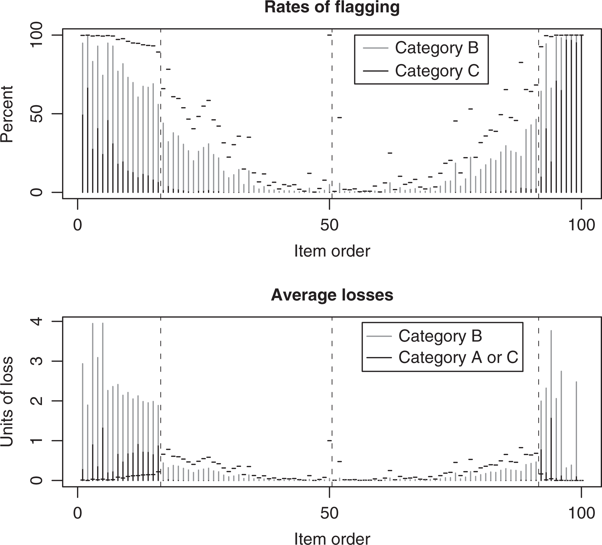
The results are presented graphically in Figure 3. In the top panel, the rates of assignment by the ABC method are represented by vertical black and gray segments for the respective categories C and B. The rates of flagging by the MEL method are marked by horizontal ticks. The items are presented in the ascending order of their values of Δ M H . The vertical dashes separate the items with Δ M H < − 1 , Δ M H > 1 and mark the zero value of Δ M H .

OPEN IN VIEWER

Figure 3.

The rates of flagging and the average losses by the ABC and MEL classifications. Simulation based on the Listening section of a test of English language proficiency; 10,000 replications.

The first item, with Δ M H = − 1.62 and s = 0.380 , is assigned to categories C, B, and A with respective rates of 49.8%, 45.1%, and 5.1%. By the MEL method, it is flagged in 99.8% of the replications. An item with Δ M H = 0.98 and s = 0.274 is assigned to categories A, B, and C with respective rates 52.5%, 44.6%, and 2.9%. Its average loss with the ABC method is between 0.029 and 0.475, depending on how we treat the assignment to category B. The average loss with MEL, 0.693, is much greater. However, an item with Δ M H = 1.15 and s = 0.438 is assigned to categories A, B, and C with comparable rates (36.6%, 53.4%, and 10.0%, respectively), but the associated loss is between 0.815 and 2.003. The expected loss with MEL is only 0.331; the item is flagged in 85% of the replications.

The MEL method has a higher rate of flagging for every item. Thus, it is more successful in identifying items with large DIF, but uniformly less successful for items with | Δ M H | < 1 . The rates of flagging of the two methods differ substantially for items with the largest standard errors s. At the extreme, the item with s = 0.914 is flagged in all replications, even though its value of Δ M H = − 0.01 is “exemplary.”

The bottom panel of Figure 3 displays the average losses for the items sorted in the same order as at the top. For high-DIF items, the average losses are much smaller with the MEL method (horizontal ticks) than due to assignments to categories A or C (vertical black segments), but for the acceptable items they are greater. Further, assignments to category B (vertical gray segments on top of the black segments) contribute to the losses, substantially so for the high-DIF items.

For the Reading section of the test, the average quadratic loss with R 0 = 2 and R 2 = 10 is 19.77, caused by 17.81 errors on average. In the ABC method, the losses due to incorrect assignment to categories A and C add up to 8.47, and the losses due to assignment to category B would add up to 39.96 if they were all regarded as incorrect. If only 29% of these losses were incurred, the average loss with the ABC method would be 20.06, slightly higher than that with MEL.

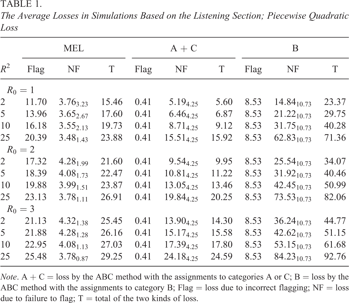
Table 1 displays the results of the simulations for piecewise quadratic loss with R ₀ = 1, 2, and 3 and R ₂ = 2, 5, 10, and 25 for the Listening section. For a setting ( R 0 , R 2 ) , the losses due to inappropriate flagging (Flag) and failure to flag (NF) and their total (T) are given for MEL method and separately for misclassifications to categories A, B, and C in ABC method. The expected total loss is listed separately for A + C and B, because some of the decisions with items assigned to category B may be correct. The average numbers of items involved in NF are given in the subscripts. For A + C and B, they are constant. They are also constant for “Flag,” and equal to the average number of items involved, because every such error is associated with unit loss.

OPEN IN VIEWER

Table 1.

The Average Losses in Simulations Based on the Listening Section; Piecewise Quadratic Loss

	MEL			A + C			B
R 2	Flag	NF	T	Flag	NF	T	Flag	NF	T
	R 0 = 1
2	11.70	3.76 3.23	15.46	0.41	5.19 4.25	5.60	8.53	14.84 10.73	23.37
5	13.96	3.65 2.67	17.60	0.41	6.46 4.25	6.87	8.53	21.22 10.73	29.75
10	16.18	3.55 2.13	19.73	0.41	8.71 4.25	9.12	8.53	31.75 10.73	40.28
25	20.39	3.48 1.43	23.88	0.41	15.51 4.25	15.92	8.53	62.83 10.73	71.36
	R 0 = 2
2	17.32	4.28 1.99	21.60	0.41	9.54 4.25	9.95	8.53	25.54 10.73	34.07
5	18.39	4.08 1.73	22.47	0.41	10.81 4.25	11.22	8.53	31.92 10.73	40.46
10	19.88	3.99 1.51	23.87	0.41	13.05 4.25	13.46	8.53	42.45 10.73	50.99
25	23.13	3.78 1.11	26.91	0.41	19.84 4.25	20.25	8.53	73.53 10.73	82.06
	R 0 = 3
2	21.13	4.32 1.38	25.45	0.41	13.90 4.25	14.30	8.53	36.24 10.73	44.77
5	21.88	4.28 1.28	26.16	0.41	15.17 4.25	15.58	8.53	42.62 10.73	51.15
10	22.95	4.08 1.13	27.03	0.41	17.39 4.25	17.80	8.53	53.15 10.73	61.68
25	25.48	3.78 0.87	29.25	0.41	24.18 4.25	24.59	8.53	84.23 10.73	92.76

Note. A + C = loss by the ABC method with the assignments to categories A or C; B = loss by the ABC method with the assignments to category B; Flag = loss due to incorrect flagging; NF = loss due to failure to flag; T = total of the two kinds of loss.

With the MEL method, the expected loss due to inappropriate flagging increases with both R 0 and R 2 , because the level of aversion to high DIF is increased. The expected loss due to failure to flag is much smaller and decreases with R 2 , as does the expected number of items involved. In contrast, the expected loss increases with R 0 . There are fewer failures to flag, but they are more costly. The total of the losses due to the two kinds of error increases with both R 0 and R 2 . The expected losses for the ABC method (A + C and B) refer to the same set of assignments, but their evaluation depends on R 0 and R 2 .

The results for simulations based on the Reading section have features very similar to those in Table 1, and are omitted.

6. Discussion

The purpose of a screening procedure is to classify each inspected item into one of the two categories. Hypothesis testing is poorly suited for this purpose because one category, which corresponds to the hypothesis, is treated as the default. Items are assigned to this category when the test fails to reject the hypothesis, without any evidence to support the hypothesis. This logical inconsistency is quite common in statistical practice. Even when it is understood, failure to reject a null hypothesis is commonly interpreted as evidence that the tested quantity is small, rarely specifying or indicating what “small” means. The current rules for DIF classification of test items at the Educational Testing Service (Dorans & Holland, 1993; Holland, 2004) ameliorate these problems by defining an intermediate category and combining the outcomes of hypothesis tests with criteria for the value of | Δ ˆ M H | .

In general, hypothesis testing does not have the capacity to take into account the consequences (ramifications) of the two kinds of error. These consequences, quantified by the loss function, are an important input in the proposed method. The method also requires a specification of what level of DIF is acceptable. Specifying the loss function and clarifying what constitutes acceptable DIF may at first seem to be difficult and contentious tasks, but in the long term, especially for regularly conducted large-scale test administrations, they are likely to contribute to greater transparency and consistency of the test construction process. The loss function and the value of δ may differ across programs or even across the groups of examinees for which DIF is assessed. They (or their plausible ranges) may be revised from time to time, to reflect the changed focus and emphasis of the test, but also the changing cognitive content of the items, abundance of their supply, and related circumstances.

We address the issue of uncertainty about the loss function by defining a range of plausible loss functions and values of δ. As a result, several decisions about each item are produced, and a course of action is proposed unequivocally only when these decisions coincide. Thus, we may reach an impasse for some items. The impasse can be resolved only by reducing the range of plausible loss functions and values of δ, or by removing the uncertainty about them altogether and declaring a single loss function. In fact, we considered only a single value of δ, 1.0. However, loss functions defined by two parameters involve 2² = 4 evaluations (and decisions) per item.

The sampling variance s 2 = v a r ( Δ ˆ M H ) is a key quantity in the MEL method. Its value is difficult to predict solely from the sizes of the reference and focal groups, and so recommendations for the sample sizes for MEL are difficult to formulate, as they are for the ABC method. The first goal might be to prevent any items from being flagged irrespective of their values of Δ ˆ M H . However, such items usually have other undesirable properties, such as being very easy or very difficult. The level of aversion to including a high-DIF item is another important factor. If the level is set extremely high, many items would be flagged. In ideal circumstances, the loss function (or its range) should be elicited from the management of the testing program, because financial costs and potential loss of good reputation are important factors. We acknowledge that this may entail commercially sensitive information.

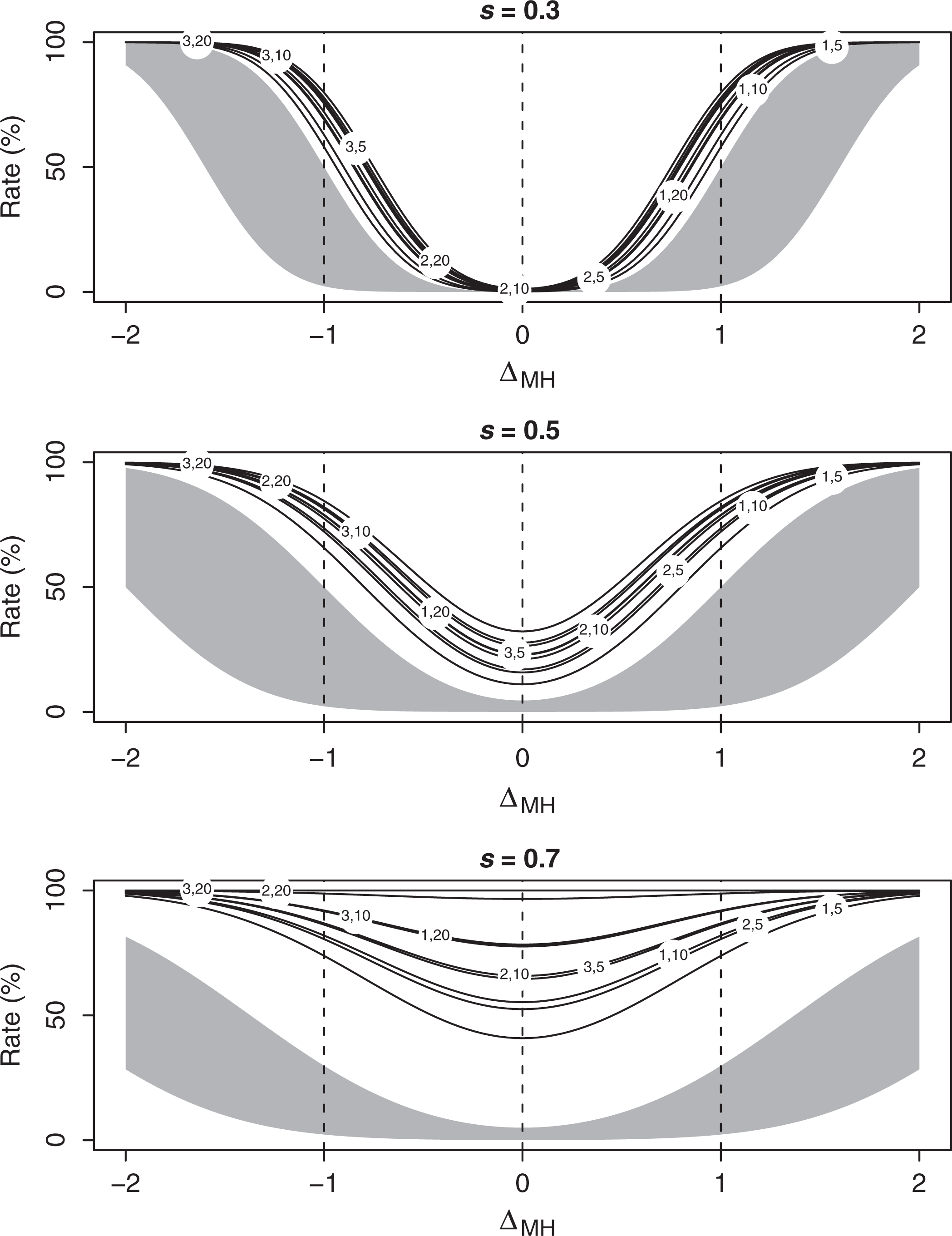
In a complementary approach, the experts would study the rates of flagging an item as functions of the item’s value of Δ M H and the standard error of its estimator, s, for a range of loss functions. These rates are evaluated directly from the normal sampling distribution N ( Δ M H , s 2 ) . Figure 4 presents these functions for s = 0.3, 0.5, and 0.7, − 2 < Δ M H < 2 and quadratic loss functions with the pairs ( R 0 , R 2 ) indicated in the panels. The curves do not intersect, and their marking is in the descending order from left to right. It confirms that the rates of flagging increase with R 0 and R 2 . For s = 0.3, the value of R 0 (1, 2, or 3) is more important for the ordering of the curves than R 2 (5, 10, or 20), but R 2 is more important for s = 0.7. The gray space in the diagram represents the rates of assigning an item to category B. That is, the white space below corresponds to the rate for category C, and the space above to the rate for category A. The diagram confirms that the MEL method has higher rates of rejection than the ABC method, uniformly so with respect to Δ M H , but the difference of the rates can be controlled by how the values of R 0 and R 2 are set. The experts are required to choose the values of R 0 and R 2 for which an appropriate balance of the two kinds of error is achieved and the value of s for which the error rates are acceptable. Converting this value of s to sample sizes is a problem shared by the ABC method.

OPEN IN VIEWER

Figure 4.

The rates of flagging as functions of Δ M H and s for a selection of piecewise quadratic loss functions given by the pairs ( R 0 , R 2 ) .

Extension of our proposal to classifying items to more than two categories is straightforward. For example, a classification with three ordered categories, such as A (acceptable DIF), B (unacceptable DIF, but not critical), and C (extremely large DIF) is formulated as two decision tasks, one to decide between A and the union of B and C, and the other between C and the union of A and B. The expected losses for the two decision tasks are added up, so that choosing A (C) when C (A) is appropriate entails two contributions to the loss. The loss functions for the two tasks have to be set, so that both of them and their total would have the property of additivity.

Analyses of data from past administrations of tests can inform the process of setting the loss function. The current and proposed screening procedures can be compared on them. The presented method has a Bayesian version which requires prior information about the distribution of Δ M H in the test. The only change that takes place is that the (frequentist) conditional distribution of Δ M H , given Δ ˆ M H and s, is replaced by its Bayesian posterior distribution for every item. Using estimated values of the parameters of this distribution corresponds to the empirical Bayes method.

Our method makes no reference to the specific form or derivation of the estimator Δ ˆ M H . Therefore, the method can be applied to other markers (statistics) that characterize DIF, or even markers for other item properties, so long as they are estimated without bias and with known sampling variances. Of course, the loss functions and the values of δ have to be revised for them—they are specific to the scale on which the marker is defined and the purpose of its use.

The computer code, written in R, for generating values involved in the table and all the figures is available from the author on request. All the evaluations except for the simulations are instant.