Handling Correlations Between Covariates and Random Slopes in Multilevel Models

Abstract

This article discusses estimation of multilevel/hierarchical linear models that include cluster-level random intercepts and random slopes. Viewing the models as structural, the random intercepts and slopes represent the effects of omitted cluster-level covariates that may be correlated with included covariates. The resulting correlations between random effects (intercepts and slopes) and included covariates, which we refer to as “cluster-level endogeneity,” lead to bias when using standard random effects (RE) estimators such as (restricted) maximum likelihood. While the problem of correlations between unit-level covariates and random intercepts is well known and can be handled by fixed-effects (FE) estimators, the problem of correlations between unit-level covariates and random slopes is rarely considered. When applied to models with random slopes, the standard FE estimator does not rely on standard cluster-level exogeneity assumptions, but requires an “uncorrelated variance assumption” that the variances of unit-level covariates are uncorrelated with their random slopes. We propose a “per-cluster regression” (PC) estimator that is straightforward to implement in standard software, and we show analytically that it is unbiased for all regression coefficients under cluster-level endogeneity and violation of the uncorrelated variance assumption. The PC, RE, and an augmented FE estimator are applied to a real data set and evaluated in a simulation study that demonstrates that our PC estimator performs well in practice.

Keywords

endogeneity hierarchical linear model multilevel model

1 Introduction

We consider linear regression models for clustered data that include cluster-specific random intercepts and slopes. Such models are called multilevel models, mixed models, random-coefficient models, or hierarchical linear models. If the models are viewed as “structural models,” the perspective taken in this article, the regression coefficients represent structural or causal parameters, and the error terms represent the effects of omitted covariates. If there are omitted confounders that are correlated with included covariates, then the error terms are correlated with the included covariates. These correlations lead to omitted variable bias. This article focuses on estimation methods that avoid bias due to omitted cluster-level confounders, also referred to as “cluster-level endogeneity.” An alternative view of models, not taken here, is that regression coefficients merely represent associations between included variables, or linear projections in the case of linear models, in which case the error terms are orthogonal to the covariates by construction (see Spanos, 2006, for a discussion of “structural” vs. “statistical” models).

Research on addressing cluster-level endogeneity in multilevel models has traditionally been confined to correlations between unit-level covariates (i.e., covariates that vary over units) and random intercepts that vary over clusters in which units are nested. This constitutes a type of “cluster-level” endogeneity, as it involves correlation with a cluster-level random error term. For instance, in estimating the effect of Catholic schooling on student achievement controlling for student socioeconomic status (SES), one may worry that school-level omitted variables, such as school resources, may be correlated with SES. Left unaddressed, this endogenity may lead us to misattribute the impacts of these omitted variables to the effect of SES. This bias may in turn spill over to other coefficients. To address this type of endogeneity, Mundlak (1978) shows that consistent estimators of the coefficients of unit-level covariates can be obtained by a fixed-effects (FE) approach. However, with standard FE estimators, coefficients of cluster-level covariates (i.e., covariates that only vary over clusters) cannot be estimated. The Hausman and Taylor (1981) instrumental variable estimator resolves this limitation and is consistent for the coefficients of both unit- and cluster-level covariates under appropriate assumptions (see Castellano, Rabe-Hesketh, & Skrondal, 2014).

Endogeneity in the form of correlations between unit-level covariates and random slopes varying over clusters may also arise. Referring back to the Catholic schooling example, when controlling for students’ SES, the slope of SES (or SES achievement gradient) may vary between schools, due to interactions between SES and omitted school-level covariates, such as school resources. If the omitted variables are negatively correlated with the SES achievement gradient, then the random slopes will be negatively correlated with SES.

Remarkably, such endogeneity is rarely considered. One exception is Frees (2004) who extends the Mundlak approach to handle random slopes. Another is Wooldridge (2005) who shows under seemingly benign conditions that traditional FE estimation of random-intercept models is robust against correlations between unit-level covariates and random slopes. However, neither of these approaches permits estimation of the coefficients of cluster-level covariates even if the covariates are exogenous (i.e., not endogenous). This limitation is overcome by Kim and Frees (2007) who use generalized method of moments estimation to extend the Hausman–Taylor approach to multilevel models with random slopes. However, their method is difficult to implement, making the FE approach more feasible in practice.

Unfortunately, a key assumption required for the FE approach may be violated in important applications. Specifically, the within-cluster variance of a unit-level covariate must be uncorrelated with the random slope of that covariate, which we refer to as the “uncorrelated variance assumption” throughout this article. Turning back to the Catholic schooling example, it is possible that more diverse schools (schools with high variance of SES) may be better equipped to mitigate the effects of SES (lower the SES achievement gradient) than schools that are more homogeneous (schools with low variance of SES). Such a situation would directly violate the uncorrelated variance assumption.

In this article, we investigate estimation of the coefficients of unit-level and cluster-level covariates in multilevel models in the presence of two sources of endogeneity; (nonzero) correlations between unit-level covariates and both the random intercept and random slopes. Throughout, we assume that covariates are uncorrelated with the unit-level error term and that cluster-level covariates are uncorrelated with the random intercepts and random slopes. We propose a simple “per-cluster regression” (PC) approach that is unbiased and consistent for coefficients of both unit-level and cluster-level covariates under both forms of cluster-level endogeneity and violation of the uncorrelated variance assumption. We contrast its performance to the “standard” random-effects (RE) estimator and what we call the “augmented FE” (FE+) approach, which extends the FE approach to provide estimates of the coefficients of cluster-level covariates. In Section 2, we first introduce our motivating empirical example and specific model of interest and then present our general model. In Section 3, we discuss the traditional RE and FE estimators and their conditions for unbiasedness. In Section 4, we introduce new estimators, namely, the FE+ estimator and the PC estimator, and show under what assumptions they are unbiased. We provide conditions for consistency for all four estimators in Online Appendix A. All estimators are applied to a data set in Section 5, and Section 6 investigates performance of the estimators using a simulation study.

2 Motivation and Multilevel Model

2.1 Motivating Example and Specific Model

As a motivating example, we consider the effect of private schooling on student achievement. We use the Raudenbush and Bryk (2002) data from the 1982 High School and Beyond (HSB) Survey because it is familiar in education and it is in the public domain, allowing us to provide data and commands for all estimators in Online Appendix B.

This two-level data set provides us with an estimation sample of 7,185 students (units) nested in 160 schools (clusters), 70 of which are Catholic (private) and the remaining of which are public. The number of observations per school ranges from 14 to 67 students (mean = 45, SD = 12). We use a mathematics standardized test score for student i in school j as our response variable, y_ij , which has a mean of 12.75 and a standard deviation of 6.88. Our primary variables of interest are w_j , a binary indicator for whether school j is Catholic, and x_ij , a continuous index of students’ SES, composed of parental education, parental occupation, and parental income. This index has a mean of 0 and a standard deviation of 0.78.

We write the model using a two-stage formulation, similar to that used in Raudenbush and Bryk (2002). The first stage is the Level-1 model:

y_{i j} = η_{0 j} + η_{1 j} x_{i j} + ε_{i j} .

This is a simple regression of the student mathematics test scores y_ij on their SES x_ij , where the intercept η_0j and slope η_1j can vary between schools, as indicated by the j subscript. Each student’s test score can deviate from the school-specific regression line by a random error term ε _ij .

The school-specific intercepts and slopes become (unobservable) outcomes in the Level-2 models:

\begin{aligned} η_{0 j} = γ_{0} + γ_{1} w_{j} + u_{0 j} \\ η_{1 j} = β_{1} + β_{2} w_{j} + u_{1 j} . \end{aligned}

The mean intercept and slope of SES, for the population of schools, depend on whether the schools are Catholic or public (w_j ). The intercepts γ₀ and β₁ in these models therefore represent the population means of the intercepts and slopes of SES for public schools, whereas the slopes γ₁ and β₂ represent the differences in population means of the intercepts and slopes between Catholic and private schools, respectively. The Level-2 models have errors u _0j and u _1j to allow the schools' intercepts and slopes to vary within the subpopulations of Catholic and private schools. Assumptions regarding the error terms are discussed in Sections 3 and 4.

Substituting the Level-2 models into the Level-1 model, we obtain the reduced form of the model:

y_{i j} = γ_{0} + γ_{1} w_{j} + β_{1} x_{i j} + β_{2} w_{j} x_{i j} + u_{0 j} + u_{1 j} x_{i j} + ε_{i j} .

We see that β₂ is the coefficient of a cross-level interaction between the student-level covariate x_ij and the school-level covariate w_j .

In this setting, it is likely that there are omitted school-level variables that affect student achievement, and hence enter the random intercept u _0j, and are correlated with student SES. If these omitted school-level variables also interact with student SES, then they enter the random slope u _1j, and the slope is then correlated with SES. Ignoring such endogeneity may lead to bias when estimating the coefficients of this model.

2.2 General Multilevel Model

The general model we consider in this article is for two-level data, such as the HSB data described previously. In the cross-sectional case, units (Level 1) are typically individuals nested within clusters (Level 2), such as schools, hospitals, or neighborhoods. In the longitudinal case, units refer to measurement occasions nested within individuals who constitute the “clusters.” Clusters are indexed j, with j = 1,…, J, and units are indexed ij, with i = 1,…, n_j . The general model includes unit-level covariates that vary between units within clusters (and between clusters) as well as cluster-level covariates that vary between clusters but are constant across units within the same cluster. Same-level and cross-level interactions may also be included, where cross-level interactions are unit-level covariates. Some unit-level covariates may have random slopes.

The general model can be written as:

y_{i} = W_{j} γ + X_{j} β + Z_{j} u_{j} + ε_{j} .

Here $y_{j} = (y_{1 j}, \dots, y_{n_{j} j})^{'}$ is the vector of responses for cluster j, the $n_{j} \times (P + 1)$ matrix W _j includes all P cluster-level covariates and its first column is a vector of ones, $1_{n_{j}}$ , for the intercept; the n_j × R matrix X _j includes all R unit-level covariates; the $n_{j} \times (R_{1} + 1)$ matrix Z _j includes all R ₁ ≤ R unit-level covariates in X _j that have random slopes and its first column is $1_{n_{j}}$ for the random intercept. Finally, the u _j are random effects or cluster-level error terms (one random intercept and R ₁ random slopes), and the ∊ _j are unit-level error terms. The u _j are assumed to be independent of the ∊ _j , and the clusters are independent in the sense that error terms as well as covariates are independent across clusters. Other required assumptions regarding u _j and ∊ _j depend on what estimators are used and are discussed in Sections 3 and 4. Sometimes all unit-level covariates have random slopes, so that R ₁ = R, but typically R ₁ < R, so that the slopes of some unit-level covariates do not vary between clusters, giving rise to the term “mixed-effects” (mixed random and “fixed” effects) model.

For the specific model of the HSB data in Equation 3, P = 1, so that W _j has n _j rows and P + 1 = 2 columns, with each row equal to (1,w_j ). The corresponding coefficients are $γ = {(γ_{0}, γ_{1})}^{'}$ . The matrix of R = 2 unit-level covariates is X _j = (x _j w_j x _j ), where $x_{j} = {(x_{1 j}, . . ., x_{n_{j} j})}^{'}$ , and $β = {(β_{1}, β_{2})}^{'} .$ The first unit-level covariate has a random slope, so $R_{1} = 1, Z_{j} = (1_{n_{j}} x_{j})$ , and $u_{j} = {(u_{0 j}, u_{1 j})}^{'}$ . Finally, the unit-level errors are $ε_{j} = {(ε_{1 j}, . . ., ε_{n_{j} j})}^{'} .$

The model in Equation 4 can be expressed more compactly by combining all covariates (i.e., X _j and W _j ) into a single matrix V _j and likewise their corresponding coefficients (β and γ) into a single vector δ:

y_{j} = V_{j} δ + Z_{j} u_{j} + ε_{j} .

It will often be convenient to stack the covariates for all J clusters in the matrix V.

Writing this general model using a two-stage formulation, analogous to Equations 1 and 2, requires additional notation, so we defer this until Section 4.2 where this formulation is useful for explaining the PC approach.

3 Standard Estimators and Conditions for Unbiasedness

3.1 Exogeneity and Endogeneity

Throughout this article, we assume unit-level exogeneity or strict exogeneity, given the random effects,

E (ε_{j} | V_{j}, u_{j}) = 0 .

It follows that $E (ε_{j} | V_{j}) = 0 a n d E (ε_{j}^{'} V_{j}) = 0$ and that each element of $ε_{j}$ is uncorrelated with each element of the covariate vectors.

The assumption of cluster-level exogeneity can be expressed as:

E (u_{j} | V_{j}) = 0 .

When this assumption is violated, there is cluster-level endogeneity.

We assume that cluster-level exogeneity holds for the cluster-level covariates

E (u_{j} | W_{j}) = 0

and discuss the problem that unit-level covariates may be cluster-level endogenous,

E (u_{j} | X_{j}) \neq 0 .

Cluster-level endogeneity occurs if, for example, $E (X_{j}^{'} 1_{n_{j}} u_{0 j}) \neq 0$ or in other words, if the cluster sums or means of the unit-level covariates are correlated with the random intercepts.

In this article, we consider RE, FE+, and (our proposed) PC approaches for estimating the model in Equation 3 when X _j is correlated with both the random intercept u _0j and the random slopes u_rj , $r = 1, . . ., R_{1} .$ In the following subsections, we describe each of these estimators and under which conditions they are unbiased for the regression coefficients $δ = {(β^{'}, γ^{'})}^{'}$ .

3.2 RE estimators

For RE estimators, the random effects, u _j , are assumed to have zero means and covariance matrix Ψ, given the covariates. They are uncorrelated across clusters, and they are also uncorrelated with the unit-level error term ∊ _j . The elements ε _ij of ∊ _j have zero means and variance θ, given the covariates, and are mutually uncorrelated.

It follows from these assumptions that the mean and covariance structure of y _j , given V _j becomes

E (y_{j} | V_{j}) = V_{j} δ,

and

Σ_{j} \equiv V a r (y_{j} | V_{j}) = Z_{j} Ψ Z_{j}^{'} + θ I_{n_{j}} .

Under the exogeneity assumptions in Equations 6 and 7, consistent estimators for the parameters of the model in Equation 5 can be obtained using maximum likelihood (ML), restricted ML (REML), or feasible generalized least squares (FGLS). The FGLS estimator can be expressed in closed form as

{\hat{δ}}_{R E} = δ + {(J^{- 1} \sum_{j = 1}^{J} V_{j}^{'} {\hat{Σ}}_{j}^{- 1} V_{j})}^{- 1} (J^{- 1} \sum_{j = 1}^{J} V_{j}^{'} {\hat{Σ}}_{j}^{- 1} (Z_{j} u_{j} + ε_{j})),

where ${\hat{Σ}}_{j}$ is an estimator of $Σ_{j},$ obtained by substituting estimators of Ψ and θ into Equation 9, and $\sum_{j} V_{j}^{'} {\hat{Σ}}_{j}^{- 1} V_{j}$ is assumed to be nonsingular with probability 1.

The conditional expectation of the GLS estimator ${\hat{δ}}_{G L S}$ (assuming ∑ is known), given V, is

E ({\hat{δ}}_{GLS} | V) = δ + {(J^{- 1} \sum_{j = 1}^{J} {V^{'}}_{j} Σ_{j}^{- 1} V_{j})}^{- 1} (J^{- 1} \sum_{j = 1}^{J} {V^{'}}_{j} Σ_{j}^{- 1} [Z_{j} E (u_{j} | V) + E (ε_{j} | V)]) .

Note that $E (ε_{j} | V) = E (ε_{j} | V_{j})$ and $E (u_{j} | V) = E (u_{j} | V_{j})$ because clusters are assumed to be independent. Furthermore, unit-level exogeneity implies that $E (ε_{j} | V_{j}) = 0$ and cluster-level exogeneity implies that $E (u_{j} | V_{j}) = 0$ . Conditional unbiasedness, $E ({\hat{δ}}_{G L S} | V) = δ$ , hence follows; and using the law of iterated expectations, ${\hat{δ}}_{G L S}$ is (unconditionally) unbiased, $E ({\hat{δ}}_{G L S}) = δ$ .

Unfortunately, due to the nonlinear nature of the FGLS estimator, this unbiasedness result does not automatically apply when estimates ${\hat{Σ}}_{j}$ are plugged in for $Σ_{j}$ . Under the previous assumptions, a sufficient assumption for unbiasedness, $E ({\hat{δ}}_{F G L S}) = δ$ , is that the error terms have symmetric distributions (Kakwani, 1967). This result also applies to ML and REML, given that these estimators can be expressed as iterative versions of the FGLS estimator (Don & Magnus, 1980). Note that for the empirical example and simulation study, we use REML, following the tradition of its use in the education research literature.

3.3 FE Estimators

In econometrics, the term fixed-effects (FE) estimator refers to an estimator that does not rely on cluster-level exogeneity, and we adopt this terminology here. Some of the estimators can be derived by treating the random effects as fixed and others by eliminating the random effects, but in either case, the effects are typically viewed as random. The traditional FE approaches have been developed for random-intercept models, with $Z_{j} = 1_{n_{j}}$ and $u_{j} = u_{0 j}$ , to handle violation of the exogeneity assumption $E (u_{0 j} | V_{j}) = 0$ (Mundlak, 1978).

We define the FE estimator in terms of the de-meaning (or group-mean centering) transformation $Q_{j} \equiv I_{n_{j}} - 1_{n_{j}} {(1_{n_{j}}^{'} 1_{n_{j}})}^{- 1} 1_{n_{j}}^{'}$ where $Q_{j} 1_{n_{j}} = 0$ , and define ${\ddot{y}}_{j} \equiv Q_{j} y_{j},$ ${\ddot{X}}_{j} \equiv Q_{j} X_{j},$ ${\ddot{Z}}_{j} \equiv Q_{j} Z_{j},$ and ${\ddot{ϵ}}_{j} \equiv Q_{j} ϵ_{j}$ . Premultiplying Equation 4 by Q _j , the de-meaned model becomes

{\ddot{y}}_{j} = {\ddot{X}}_{j} β + {\ddot{Z}}_{j} u_{j} + {\ddot{ϵ}}_{j} .

Note that ${\ddot{W}}_{j} γ = 0_{n_{j}}$ because the columns of W _j are constant. The first column of ${\ddot{Z}}_{j}$ is $0_{n_{j}}$ because the first column of Z _j is $1_{n_{j}}$ , so that the random part of the model does not depend on $u_{0_{j}}$ . The FE estimator can be obtained by applying a pooled ordinary least squares (POLS) estimator (pooling over the Level-2 units) to the de-meaned model, giving

{\hat{β}}_{F E} = β + {(J^{- 1} \sum_{j = 1}^{J} {\ddot{X}}_{j}^{'} {\ddot{X}}_{j})}^{- 1} (J^{- 1} \sum_{j = 1}^{J} {\ddot{X}}_{j}^{'} ({\ddot{Z}}_{j} u_{j} + {\ddot{ϵ}}_{j})),

where $\sum_{j} {\ddot{X}}_{j}^{'} {\ddot{X}}_{j}$ is assumed to be nonsingular with probability 1.

To derive the conditions for unbiasedness, stack the ${\ddot{X}}_{j}$ for all clusters j in $\ddot{X}$ . Consider the conditional expectation of ${\hat{β}}_{F E}$ , given $\ddot{X}$ ,

E ({\hat{β}}_{F E} | \ddot{X}) = β + {(J^{- 1} \sum_{j = 1}^{J} {\ddot{X}}_{j}^{'} {\ddot{X}}_{j})}^{- 1} (J^{- 1} \sum_{j = 1}^{J} {\ddot{X}}_{j}^{'} [{\ddot{Z}}_{j} E (u_{j} | \ddot{X}) + E ({\ddot{ϵ}}_{j} | \ddot{X})]) .

Keep in mind that ${\ddot{Z}}_{j}$ is a subset of ${\ddot{X}}_{j}$ and note that $E (u_{j} | \ddot{X}) = E (u_{j} | {\ddot{X}}_{j})$ and $E ({\ddot{ϵ}}_{j} | \ddot{X}) = E ({\ddot{ϵ}}_{j} | {\ddot{X}}_{j})$ because clusters are independent. Furthermore, unit-level exogeneity implies that $E (\ddot{ϵ} | {\ddot{X}}_{j}) = 0$ , and cluster-level exogeneity implies that $E (u_{j} | {\ddot{X}}_{j}) = 0$ , so ${\hat{β}}_{F E}$ is conditionally unbiased, $E ({\hat{β}}_{F E} | \ddot{X}) = β$ . Finally, using the law of iterated expectations, it follows that ${\hat{β}}_{F E}$ is (unconditionally) unbiased, $E ({\hat{β}}_{F E}) = β$ .

Wooldridge (2005, 2010, section 11.7.3) considers FE estimation for a special case of Equation 4 without cluster-level covariates W _j . He derives the conditions required for consistency of the traditional FE estimator, and we briefly derive the analogous results for the general model (Equation 4) in Online Appendix A, Section A.2. The condition for consistency plim ${\hat{β}}_{F E} = β$ , is

E ({\ddot{X}}_{j}^{'} {\ddot{Z}}_{j} u_{j}) = 0 .

As pointed out by Wooldridge (2010, p. 382), this assumption allows u _j to be correlated with the “permanent” components of X _j , but not the “idiosyncratic” components ${\ddot{X}}_{j}$ . Condition 12 is implied by the more easily interpretable condition for unbiasedness,

E (u_{j} | \ddot{X_{j}}) = 0,

because $E ({\ddot{X}}_{j}^{'} {\ddot{Z}}_{j} u_{j} | {\ddot{X}}_{j}) = {\ddot{X}}_{j}^{'} {\ddot{Z}}_{j} E (u_{j} | {\ddot{X}}_{j}) .$

We now look at the assumption in Equation 12, which is required for consistency and unbiasedness, in more detail for our specific model for the empirical example in Equation 3 to understand how it can be violated. In that model, ${\ddot{X}}_{j} = ({\ddot{x}}_{j} w_{j} {\ddot{x}}_{j})$ and ${\ddot{Z}}_{j} = (0_{n_{j}} {\ddot{x}}_{j})$ . The condition can be written as two nontrivial equations,

E [(\begin{matrix} {\ddot{x}}_{j}^{'} \\ w_{j} {\ddot{x}}_{j}^{'} \end{matrix}) {\ddot{x}}_{j} u_{1 j}] = 0 .

Concentrating on the first equation, we obtain

E ({\ddot{x}}_{j}^{'} {\ddot{x}}_{j} u_{1 j}) = E [(\sum_{i = 1}^{n_{j}} {\ddot{x}}_{i j}^{2}) u_{1 j}] = (n_{j} - 1) E (s_{j}^{2} u_{1 j}) = 0,

where $s_{j}^{2}$ is the sample variance of x_ij for cluster j. In other words, the condition is violated if the within-cluster variance of x_ij is correlated with the random slope u _1j. In our empirical example, it seems reasonable that more diverse schools (larger $s_{j}^{2}$ ) may be better suited to mitigate the effects of SES (smaller u _1j) than more homogeneous schools. We will therefore consider the problem of nonzero correlation between the within-cluster variance of x_ij and its random slope u _1j and will refer to Equation 12 as the “uncorrelated variance assumption.” Note, however, that Equation 12 can also be violated in other ways. For instance, in longitudinal data, the covariate value at the initial time point, x _1j, may be correlated with u _1j.

4 New Estimators and Conditions for Unbiasedness

4.1 FE+ Estimator

The FE approach does not permit estimation of the coefficients, γ, of any cluster-level covariates, but it can be “augmented” so that it does. The FE+ estimator we use is similar to the estimator proposed by Hausman and Taylor (1981) to estimate effects of cluster-level covariates for two-level models with only random intercepts—and no random slopes. As pointed out by Castellano, Rabe-Hesketh, and Skrondal (2014), the estimator discussed here has been invented and reinvented several times (e.g., Ballou, Sanders, & Wright, 2004; Raudenbush & Willms, 1995; Wiley, 1975). However, the conditions for unbiasedness for random-coefficient models have not previously been considered.

Step 1: Estimation of β

In the first step, β (coefficients for all unit-level covariates) is estimated by FE. The estimator is unbiased under the uncorrelated variance assumption in Equation 12 and the unit-level exogeneity assumption in Equation 6.

Step 2: Estimation of γ

In the second step, we obtain quasi-residuals r _j ,

r_{j} \equiv y_{j} - X_{j} {\hat{β}}_{F E},

and estimate γ (coefficients for the cluster-level covariates) in the regression of r _j on W _j by POLS. Substituting Equation 4 for y _j , we obtain

r_{j} = W_{j} γ + X_{j} (β - {\hat{β}}_{F E}) + Z_{j} u_{j} + ϵ_{j} .

The POLS estimator of γ can be expressed as

\hat{γ} = γ + {(J^{- 1} \sum_{j = 1}^{J} {W^{'}}_{j} W_{j})}^{- 1} (J^{- 1} \sum_{j = 1}^{J} {W^{'}}_{j} [X_{j} (β - {\hat{β}}_{F E}) + Z_{j} u_{j} + ϵ_{j}]),

where $\sum_{j} {W^{'}}_{j} W_{j}$ is assumed to be nonsingular with probability 1.

The conditional expectation of the POLS estimator $\hat{γ}$ given $V$ , becomes

E (\hat{γ} | V) = γ + {(J^{- 1} \sum_{j = 1}^{J} {W^{'}}_{j} W_{j})}^{- 1} (J^{- 1} \sum_{j = 1}^{J} {W^{'}}_{j} {X_{j} [β - E ({\hat{β}}_{FE} | V)] + Z_{j} E (u_{j} | V) + E (ε_{j} | V)}) .

Conditional unbiasedness, $E (\hat{γ} | V) = γ$ follows since (i) $E ({\hat{β}}_{F E} | V)] = β$ under the uncorrelated variance assumption, (ii) $E (u_{j} | V) = E (u_{j} | V_{j})$ and $E (ϵ_{j} | V) = E (ϵ_{j} | V_{j})$ due to independence of the clusters, and (iii) $E (u_{j} | V_{j}) = 0$ and $E (ϵ_{j} | V_{j}) = 0$ under the exogeneity assumptions. Using the law of iterated expectations, we finally obtain (unconditional) unbiasedness $E (\hat{γ}) = γ .$

To implement the FE+ approach for the empirical example, the two steps are as follows: (1) estimate β₁ and β₂ by FE and (2) regress quasi-residuals, $r_{i j} \equiv y_{i j} - {\hat{β}}_{1 F E} x_{i j} - {\hat{β}}_{2 F E} w_{j} x_{i j}$ , on w_j to obtain estimates of γ₀ and γ₁.

4.2 PC estimator

In this section, we define our proposed PC estimator. This estimator is best understood by using the two-stage formulation (see Section 2.1) of the general model in Equation 4, which requires some new notation.

The columns of the matrix X _j of unit-level covariates can be ordered, so that the matrix can be decomposed as $X_{j} = (X_{1 j} X_{2 j} X_{3 j})$ , where X _1j contains the R ₁ unit-level covariates that have random slopes, so that $Z_{j} = (1_{n_{j}} X_{1 j})$ , X _2j are R ₂ cross-level interactions between unit-level covariates in X _1j, and cluster-level covariates in W _j , and X _3j are the R ₃ remaining unit-level covariates (which may include cross-level interactions between covariates in W _j and other covariates in X _3j). Correspondingly, $β = (β_{1}^{'}, β_{2}^{'}, β_{3}^{'})$ and $R = R_{1} + R_{2} + R_{3}$ . The two-stage model can then be written as

y_{j} = X_{3 j} β_{3} + Z_{j} η_{j} + ϵ_{j},

η_{r j} = w_{r j}^{^{'}} α_{r} + u_{r j}, r = 0, \dots, R_{1},

where η _j are cluster-specific coefficients. Here, Equation 15 is referred to as the Level-1 or unit-level model, and Equation 16 for the R ₁ + 1 cluster-specific coefficients of the Level-1 model is referred to as the Level-2 or cluster-level model. When r = 0, Equation 16 is the model for the cluster-specific intercept η_0j, ${w^{'}}_{0 j}$ is a row of W _j (with $W_{j} = 1_{n_{j}} \otimes {w^{'}}_{0 j}$ ) and α₀ = γ. When r > 0 , Equation 16 is the model for the cluster-specific slope of the rth column of X _1j. The vector w _rj includes only those cluster-level covariates that interact with the rth column of X _1j. The first element of α _r is β_1r and the other elements are subsets of β₂. Note that we include Level-2 models only for the coefficients of those unit-level covariates that have random slopes.

Equations 15 and 16 are a generalization of the two-stage formulation of the model for the HSB example in Equations 1 and 2. In that model, there are R ₁ = 1 covariates X _1j = x _j with random slopes and β₁ = β₁. There are also R ₂ = 1 cross-level interactions between unit-level covariates in X _1j and a cluster-level covariate w_j , namely X _2j = w_j x _j with β₂ = β₂. There are no remaining columns of X _j , so R ₃ = 0, and there is no X _3j or β₃. Further, $η_{j} = {(η_{0 j}, η_{1 j})}^{'},$ $w_{0 j} = w_{1 j} = {(1, w_{j})}^{'}$ , $α_{0} = {(γ_{0}, γ_{1})}^{'}$ , and $α_{1} = {(β_{1}, β_{2})}^{'}$ . We now outline the steps for our proposed PC estimator.

Step 1: Estimation of β₃

Wooldridge (2005, 2010, section 11.7.2) considers the special case of this model without cluster-level covariates, that is, with $η_{j} = β_{1} + u_{j}$ , and describes estimation of β₃ (coefficients for all unit-level covariates without random slopes) by an extension of the de-meaning transformation used in FE estimation. Instead of premultiplying by the de-meaning operator $Q_{j}$ , we premultiply the Level-1 model by the projection matrix

M_{j} \equiv I_{n_{j}} - Z_{j} {({Z^{'}}_{j} Z_{j})}^{- 1} {Z^{'}}_{j} .

Defining ${\dot{y}}_{j} = M_{j} y_{j}$ , ${\dot{X}}_{3 j} = M_{j} X_{3 j}$ , and ${\dot{ϵ}}_{j} = M_{j} ϵ_{j}$ , and noting that ${\dot{Z}}_{j} = M_{j} Z_{j} = 0$ , gives

{\dot{y}}_{j} = {\dot{X}}_{3 j} β_{3} + ϵ_{j} .

The POLS estimator of β₃, denoted ${\hat{β}}_{3 C M L}$ , can be expressed as

{\hat{β}}_{3 C M L} = β_{3} + {(J^{- 1} \sum_{j = 1}^{J} {\dot{X}}_{3 j}^{'} {\dot{X}}_{3 j})}^{- 1} (J^{- 1} \sum_{j = 1}^{J} {\dot{X}}_{3 j}^{'} {\dot{ϵ}}_{j}),

where $\sum_{j} {\dot{X}}_{3 j}^{'} {\dot{X}}_{3 j}$ is assumed to be nonsingular with probability 1. If the $ε_{i j}$ are normally distributed, this estimator also corresponds to the conditional ML (CML) estimator, conditioning on the sufficient statistics ${Z_{j}}^{'} y_{j}$ for the “nuisance parameters” η _j (Verbeke, Spiessens, & Lesaffre, 2001).

The conditional expectation of ${\hat{β}}_{3 C M L}$ , given all covariates V, becomes

E ({\hat{β}}_{3 C M L} | V) = β_{3} + {(J^{- 1} \sum_{j = 1}^{J} {\dot{X}}_{3 j}^{'} {\dot{X}}_{3 j})}^{- 1} (J^{- 1} \sum_{j = 1}^{J} {\dot{X}}_{3 j}^{'} E ({\dot{ϵ}}_{j} | V)) .

Unit-level exogeneity, which implies that $E ({\dot{ϵ}}_{j} | V) = 0$ , is a sufficient condition for conditional unbiasedness $E ({\hat{β}}_{3 C M L} | V) = β_{3}$ .

Step 2: Estimation of η _j

Next, form quasi-residuals as

r_{j} \equiv y_{j} - X_{3 j} {\hat{β}}_{3 C M L}

and then obtain OLS estimates ${\overset{⌣}{η}}_{j}$ for the regressions of r _j on Z _j for each cluster, $j = 1, . . ., J$ ,

{\overset{⌣}{η}}_{j} = {(Z_{j} {Z^{'}}_{j})}^{- 1} {Z^{'}}_{j} r_{j} = {(n_{j}^{- 1} \sum_{i = 1}^{n_{j}} z_{i j} {z^{'}}_{i j})}^{- 1} (n_{j}^{- 1} \sum_{i = 1}^{n_{j}} z_{i j} r_{i j}),

where $z_{i j}^{'}$ is the ith row of Z _j , and $\sum_{i = 1}^{n_{j}} z_{i j} z_{i j}^{'}$ is nonsingular with probability 1, which requires that $R_{1} + 1 \leq n_{j}$ . This step gives rise to the name PCs. Identical estimates of β ₃ and η _j are obtained by treating η _j as fixed parameters in Equation 15 via the inclusion of dummy variables for the clusters and interactions between these dummy variables and the columns of Z _j .

The estimator in Equation 17 can alternatively be expressed as

{\overset{⌣}{η}}_{j} = η_{j} + {(Z_{j} {Z^{'}}_{j})}^{- 1} {Z^{'}}_{j} [X_{3 j} (β_{3} - {\hat{β}}_{3 CML}) + ε_{j}],

and the conditional expectation of ${\overset{⌣}{η}}_{j}$ , given V, becomes

E ({\overset{⌣}{η}}_{j} | V) = η_{j} + {(Z_{j} {Z^{'}}_{j})}^{- 1} {Z^{'}}_{j} {X_{3 j} [β_{3} - E ({\hat{β}}_{3 CML} | V)] E (ε_{j} | V)},

where $Z_{j} {Z_{j}}^{'}$ is assumed to be nonsingular with probability 1. Because $E ({\hat{β}}_{3 C M L} | V) = β_{3}$ from Step 1, it follows that $X_{3 j} [β_{3} - E ({\hat{β}}_{3 C M L} | V)] = 0$ . It follows from unit-level exogeneity that $E (ϵ_{j} | V) = 0$ , and therefore ${\overset{⌣}{η}}_{j}$ is conditionally unbiased, $E ({\overset{⌣}{η}}_{j} | V) = η_{j}$ .

Step 3: Estimation of γ, β₁, and β₂

The remaining regression coefficients γ (for cluster-level covariates), β₁ (for unit-level covariates with random slopes), and β₂ (for cross-level interactions involving unit-level covariates with random slopes) are now estimated. These coefficients are contained in the vectors α _r , $r = 0, . . ., R_{1}$ , in Equation 16. We write each Level-2 equation for all clusters using the following vector notation. Let $η_{r}^{*} = (η_{r 1}, \dots, η_{r J})^{'}$ and $u_{r}^{*} = {(u_{r 1}, \dots, u_{r J})}^{'}$ and let $W_{r}^{*}$ have J rows $w_{r j}^{'}$ , $j = 1, \dots, J$ . The Level-2 equation for each $η_{r}^{*}$ can then be written as

η_{r}^{*} = W_{r}^{*} α_{r} + u_{r}^{*}, r = 0, \dots, R_{1} .

Denoting the vector of estimates $η_{r}^{*} \equiv {({\overset{⌣}{η}}_{r 1},. . ., {\overset{⌣}{η}}_{r J})}^{'}$ , the model can be written as

η_{r}^{*} = W_{r}^{*} α_{r} + u_{r}^{*} + {\overset{⌣}{η}}_{r}^{*} - η_{r}^{*}

We estimate α _r by applying OLS to the regression of $η_{r}^{*}$ on $W_{r}^{*}$ , giving

\begin{matrix} {\hat{α}}_{r} = α_{r} + {(W_{r}^{*} W_{r}^{*})}^{- 1} W_{r}^{*} (u_{r}^{*} + {\overset{⌣}{η}}_{r}^{*} - η_{r}^{*}) \\ = α_{r} + {(J^{- 1} \sum_{j = 1}^{J} w_{r j} {w^{'}}_{r j})}^{- 1} (J^{- 1} \sum_{j = 1}^{J} w_{r j} (u_{r j} + {\overset{⌣}{η}}_{r j} - η_{r j})), \end{matrix}

where, for each r, $\sum_{j} w_{r j} {w^{'}}_{r j}$ is assumed to be nonsingular with probability 1.

The conditional expectation of ${\hat{α}}_{r}$ , given V, is given by:

E ({\hat{α}}_{r} | V) = α_{r} + {(J^{- 1} \sum_{j = 1}^{J} w_{r j} {w^{'}}_{r j})}^{- 1} (J^{- 1} \sum_{j = 1}^{J} w_{r j} [E (u_{r j} | V) + E ({\overset{⌣}{η}}_{r j} | V) - η_{r j}]) .

It follows from cluster-level exogeneity that $E (u_{r j} | V) = 0$ and from the results for Step 2 that $E ({\overset{⌣}{η}}_{r j} | V) = η_{r j}$ . Hence, $E ({\hat{α}}_{r} | V) = α_{r}$ , and using the law of iterated expectations, we see that the estimator is unbiased; $E ({\hat{α}}_{r}) = α_{r}$ .

For the special case of our model with $η_{j} = β_{1} + u_{j}$ , the estimator for β becomes the sample mean of ${\overset{⌣}{η}}_{r}^{*}$ , and that estimator has been proposed by Wooldridge (2010, equation 11.80). In models in which $X_{j} = (X_{1 j} X_{2 j})$ , or R ₃ = 0, the first step can be skipped and $r_{j} = y_{j}$ . Our empirical illustration is an example of the latter special case. Accordingly, we first estimate η _0j and η _1j in Equation 2 for each cluster j by regressing $y_{j}$ on $x_{j}$ using OLS, giving unbiased estimates ${\overset{⌣}{η}}_{0 j}$ and ${\overset{⌣}{η}}_{1 j}$ . Identical estimates are obtained by OLS with dummy variables for clusters and interactions between these dummy variables and x_ij . Next, ${\overset{⌣}{η}}_{0 j}$ and ${\overset{⌣}{η}}_{1 j}$ are both regressed on w_j using OLS. In the regression for ${\overset{⌣}{η}}_{0 j}$ , the OLS estimator for the intercept is unbiased for γ₀ and the OLS estimator for the coefficient of w_j is unbiased for γ₁. In the regression for ${\overset{⌣}{η}}_{1 j}$ , the OLS estimator for the intercept is unbiased for β₁ and the OLS estimator for the coefficient of w_j is unbiased for β₂. If we did not include the cross-level interaction term, x_ijw_j , in our model, there would be no β₂, $R_{1} = R$ , and we would regress ${\overset{⌣}{η}}_{1 j}$ on just the intercept, that is, find its sample mean, to obtain the unbiased estimate of β₁.

5 Empirical Example

To ground comparisons of our estimators of interest, we apply each to the HSB data introduced in Section 2.1. Table 1 provides estimates of the regression coefficients for Equation 3. All estimates were obtained using standard commands in Stata 13 (StataCorp, 2013), such as mixed and xtreg (see Online Appendix B). Note that the RE estimate of the correlation between the random intercept and slope is 1, a relatively frequent occurrence in random-coefficient models (Chung, Gelman, Rabe-Hesketh, Liu, & Dorie, In press).

Table 1

Estimates of Regression Coefficients From Different Methods For HSB Data

	Random Effects (RE)		Augmented Fixed Effects (FE+)		Per-Cluster Regression (PC)
	Estimates	(SE)	Estimates	(SE)	Estimates	(SE)
γ₀ [Constant]	11.752	(0.232)	11.769	(0.205)	11.615	(0.271)
γ₁ [Catholic]	2.130	(0.346)	2.186	(0.337)	2.253	(0.406)
β₁ [SES]	2.958	(0.143)	2.782	(0.145)	2.772	(0.169)
β₂ [SES × Catholic]	−1.313	(0.216)	−1.349	(0.218)	−1.303	(0.234)

Note. All estimates are significantly different from 0 at the 0.05 level. HSB = high school and beyond.

Castellano et al. (2014) show that positive correlation between a random intercept and a student-level covariate leads to overestimation of the coefficient of the covariate. Indeed, from the HSB data results presented in Table 1, we see that RE produces the largest estimate of the coefficient of SES, 2.958, approximately 6% higher than the closest estimate (FE+). The indicator variable w_j for Catholic schools is positively correlated with SES and therefore overestimation of the coefficient of SES is accompanied by underestimation of the coefficient of w_j , with RE producing the smallest estimate of γ₁, at 2.130.

While the differences in the FE+ and RE estimates of γ₁ may be practically significant, they are close in magnitude to the estimated standard errors (SEs) of the coefficient estimates. FE+ produces estimates of both β₁ and γ₁ that lie between the estimates produced by RE and PC, which is intuitive, given that FE+ relies only on the uncorrelated variance assumption, whereas RE additionally requires exogeneity, and PC requires neither assumption. PC gives the smallest estimated effect of SES on math achievement scores ( ${\hat{β}}_{1} = 2.772$ ) and the largest estimated effect of Catholic schooling ( ${\hat{γ}}_{1} = 2.253$ ). These estimates differ by about 6% from the RE counterparts, enough to give practitioners pause.

The small difference between estimates of β₁ from FE+ and PC suggests that the within-school variance in SES is not strongly correlated with the random slope. In fact, the within-school standard deviation of SES has a correlation of only 0.04 with the estimated residuals from the regression of ${\overset{⌣}{η}}_{1 j}$ on w_j in the final step of the PC approach.

6 Simulation Study

We now conduct a simulation study to investigate the performance of the RE, FE+, and PC estimators. In particular, we are interested in the amount of bias for RE and FE+ when the respective assumptions of cluster-level exogeneity and uncorrelated variance are violated. We also evaluate all three estimators, RE, FE+, and PC, by their root mean square errors (RMSEs) and consider performance of the estimated SEs. We use Stata 13 (StataCorp, 2013) throughout.

6.1 Data Generation Process

We generate the data using our model of interest in Equation 3. We first draw the school-level variables for each of J = 100 clusters. The random intercepts u _0j and random slopes u _1j are drawn from a bivariate normal distribution with zero means and variance–covariance matrix defined by variances ψ₀ = 0.4² and ψ₁ = 0.25² and correlation ρ = 0.5, giving the covariance ψ₁₀ = 0.05. We specify these variances to reflect those found in our empirical example. The exogenous school-level covariate w_j is drawn independently from a normal distribution with mean 1.7 and variance $σ_{w}^{2} = 1$ .

We then generate the student-level covariate x_ij as

x_{i j} = b_{0} u_{0 j} + b_{1} u_{1 j} + b_{2} w_{j} + a e_{i j}, e_{i j} ~ N (0, σ_{j}),

where

a = \sqrt{1 - ψ_{0} b_{0}^{2} - ψ_{1}^{2} b_{1}^{2} - σ_{w}^{2} b_{2}^{2} - 2 b_{0} b_{1} ψ_{10}} .

Here, b ₀ = 1.33, b ₁ = 2.13, and b ₂ = 0.20, so that $x_{i j}$ is positively correlated with the random intercept, random slope, and school-level covariate w_j . Finally, we generate y_ij according to Equation 3 with γ₀ = 1, γ₁ = 3, β₁ = 1, and β₂ = 2.

The key assumption under which we want to assess the performance of the competing estimators is that the sample within-cluster variance $s_{j}^{2}$ of x_ij is uncorrelated with the random slope u _1j. Thus, the population within-cluster standard deviation σ _j is of particular importance. Accordingly, the uncorrelated variance assumption factor in this simulation has two levels: when it holds, σ _j = 1, and when it is violated, σ _j = exp(u _1j).

Although our empirical example involves schools that tend to have large numbers of students, both RE and FE are commonly used with classrooms serving as clusters. Furthermore, there are numerous relevant applications with longitudinal data where we often find even smaller cluster sizes. Thus, we also vary cluster size, primarily considering cluster sizes of 4 and 20. For simplicity, we set cluster sizes equal across clusters, n_j = n. We fully cross the cluster size and uncorrelated variance assumption factors, yielding four primary simulation conditions defined by (large/small n) × (uncorrelated variance assumption holds/violated). To further determine the effect of cluster size when the uncorrelated variance assumption is violated, we also consider a range of cluster sizes from 4 to 50: n = 4, 8, 14, 20, 50.

All conditions are replicated 500 times. Due to occasional lack of variation of x_ij within some small clusters, the PC approach fails for some replications. The lowest number of successful replications is 489, which occurs when the variance of x_ij is correlated with the random slopes, and we have only four observations in each cluster. For all simulation conditions with a cluster size of 20, all 500 replications are successful.

6.2 Results

We evaluate the performance of each of our three estimators (RE, FE+, and PC) of the fixed regression coefficients in our model of interest (Equation 3) across our four simulation conditions. The estimated bias and RMSE are given in Table 2. Online Appendix C provides supplemental tables for each coefficient that also include the mean SEs, standard deviations of the estimates, and the ratios of these values.

Table 2

Comparing Methods for Estimating the Coefficients Using Simulated Data

		β₁ [ $x_{i j}$ ]		β₂ [ $x_{i j} \times w_{j}$ ]		γ₁ [w_j ]
Simulation		100×	100×	100×	100×	100×	100×
Condition	Method	Bias	RMSE	Bias	RMSE	Bias	RMSE
Small clusters and uncorrelated variance	RE	16.6*	21.6	0.8	7.0	−4.5*	8.0
	FE+	0.6	16.2	0.0	8.2	−0.3	7.4
	PC	1.9	25.5	−0.6	13.3	−0.5	12.7
Small clusters and correlated variance	RE	21.3*	24.2	1.2	6.1	−5.3*	8.2
	FE+	11.7*	19.1	0.2	7.9	−2.4*	8.2
	PC	−1.8	26.7	0.7	13.4	0.2	12.2
Large clusters and uncorrelated variance	RE	6.2*	10.0	0.2	3.9	−1.7*	4.9
	FE+	−0.3	8.0	0.2	4.0	0.2	5.3
	PC	−0.2	8.0	0.1	4.1	0.0	5.2
Large clusters and correlated variance	RE	12.6*	14.4	−0.1	3.5	−2.9*	5.2
	FE+	12.8*	15.2	−0.3	4.2	−2.5*	5.2
	PC	0.7	7.7	−0.3	4.0	0.0	5.0

Note. RMSE = root mean square error; RE = random effects; FE+ = augmented fixed effects; PC = per-cluster regression; small clusters: n_j = n = 4, large clusters: n_j = n = 20; uncorrelated variance: $σ_{j}^{2} = 1$ , correlated variance: $σ_{j} = exp (u_{1 j})$ .

*Estimated bias differs significantly from 0 at the 0.05 level.

6.2.1 Bias

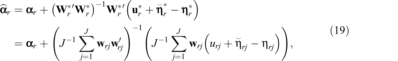
For β₁, the coefficient of the endogenous student-level covariate x_ij , there are three main results. First, the PC estimator is unbiased across all conditions even when the uncorrelated variance assumption is violated. Figure 1 clearly illustrates this finding as the empirical distributions of the errors (i.e., estimate − parameter) of the PC estimator (the solid curves) are centered on 0 in all four panels, where each panel represents one of the four simulation conditions.

Figure 1.

Kernel density plots of estimation errors, ${\hat{β}}_{1} - β_{1}$ , for coefficient of x_ij across replications for all methods when the uncorrelated variance assumption holds (left panels) and when it is violated (right panels). Note. FE+ = augmented fixed effects; PC = per-cluster regression; RE = random effects.

Second, the RE estimator is biased regardless of whether the uncorrelated variance assumption holds, whereas the FE+ estimator is biased only when this assumption is violated. This result for RE is expected, given that the RE estimator relies on the assumption of both unit- and cluster-level exogeneity (see Section 3.2), and cluster-level exogeneity is violated in all four conditions, with the nonzero correlation between x_ij and both the random intercept and its random slope. We do note, however, that violation of the uncorrelated variance assumption exacerbates the magnitude of the RE estimator’s bias: For the small cluster size condition (n = 4), the estimated bias is 1.28 times as large; and for the larger cluster size (n = 20), the estimated bias more than doubles as shown in the first column of results in Table 2. In contrast, the FE+ approach only requires unit-level exogeneity assumptions and thus produces unbiased estimates under cluster-level endogeneity as long as there is no correlation between the random slopes and within-cluster variance of x_ij . This is evident in Figure 1 by observing that the curves for FE+ (dashed) are more similar to those for PC (solid) in the left-hand plots (for uncorrelated variance simulation conditions) and more similar to the curves for RE (dot-dashed) in the right-hand plots (for correlated variance simulation conditions).

Third, the estimated bias for β₁ is larger than that for the other two regression coefficients, which is not surprising, given that x_ij is the source of the endogeneity. For instance, as shown in Table 2, the estimated bias of ${\hat{β}}_{1 R E}$ ranges from 6.2% to 21.3% of the true value. The next largest estimated bias is −0.053 for ${\hat{γ}}_{1 R E}$ under the small clusters and uncorrelated variance condition, which is only 1.8% of the coefficient’s true value (γ₁ = 3).

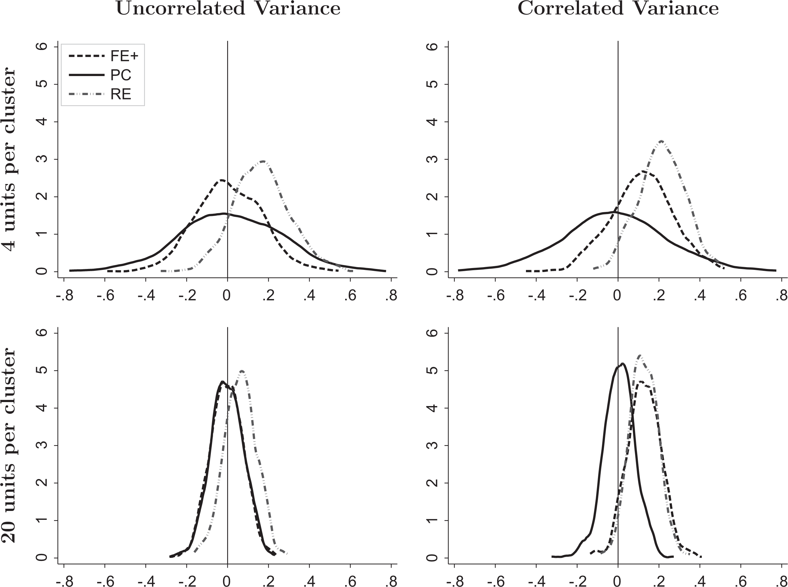
The coefficient of the interaction term, β₂, is the least affected by the simulation conditions. We only find statistically significant bias (at the 5% level) for ${\hat{β}}_{2 R E}$ for the small cluster size condition—both when the uncorrelated variance assumption holds and when it is violated. Even in these cases, as given in Table 2, the estimated bias is rather small relative to the magnitude of the true value (β₂ = 2): It is 0.4% of the parameter value when the condition holds and 0.6% when it is violated. (Plots of the empirical distributions of the estimation errors for β₂ are given in Figure C.1 in Online Appendix C.)

The estimated biases of the estimators for the coefficient γ₁ of the exogenous school-level covariate w_j follow similar patterns as for the coefficient β₁ of the endogenous student-level covariate x_ij . Just as for β₁, the PC estimator is unbiased across all conditions, the FE+ estimator is biased only when the variance of x_ij is correlated with the random slope u _1j (i.e., uncorrelated variance assumption violated), and the RE estimator is biased regardless of whether the uncorrelated variance assumption is violated. These findings are clearly illustrated in Figure 2 by comparing the centers of the empirical distributions of errors for all estimators across all conditions: the PC curve (solid) is always centered on 0, whereas the RE curve (dot-dashed) is always centered below 0, and the FE+ curve (dashed) is centered below 0 only for the correlated variance conditions in the right-hand panels. Just as with β₁, the FE+ estimator’s bias for γ₁ does not vary with cluster size—its estimate is about 0.8% of the true parameter value for both n = 4 and n = 20 as seen in Table 2. Cluster size affects the RE estimator’s bias for γ₁, as it did for β₁: As cluster size increases, the bias decreases. When the uncorrelated variance assumption holds, this bias decreases by about 63% going from n = 4 to n = 20, and by about 45% when the assumption is violated (see Table 2).

Figure 2.

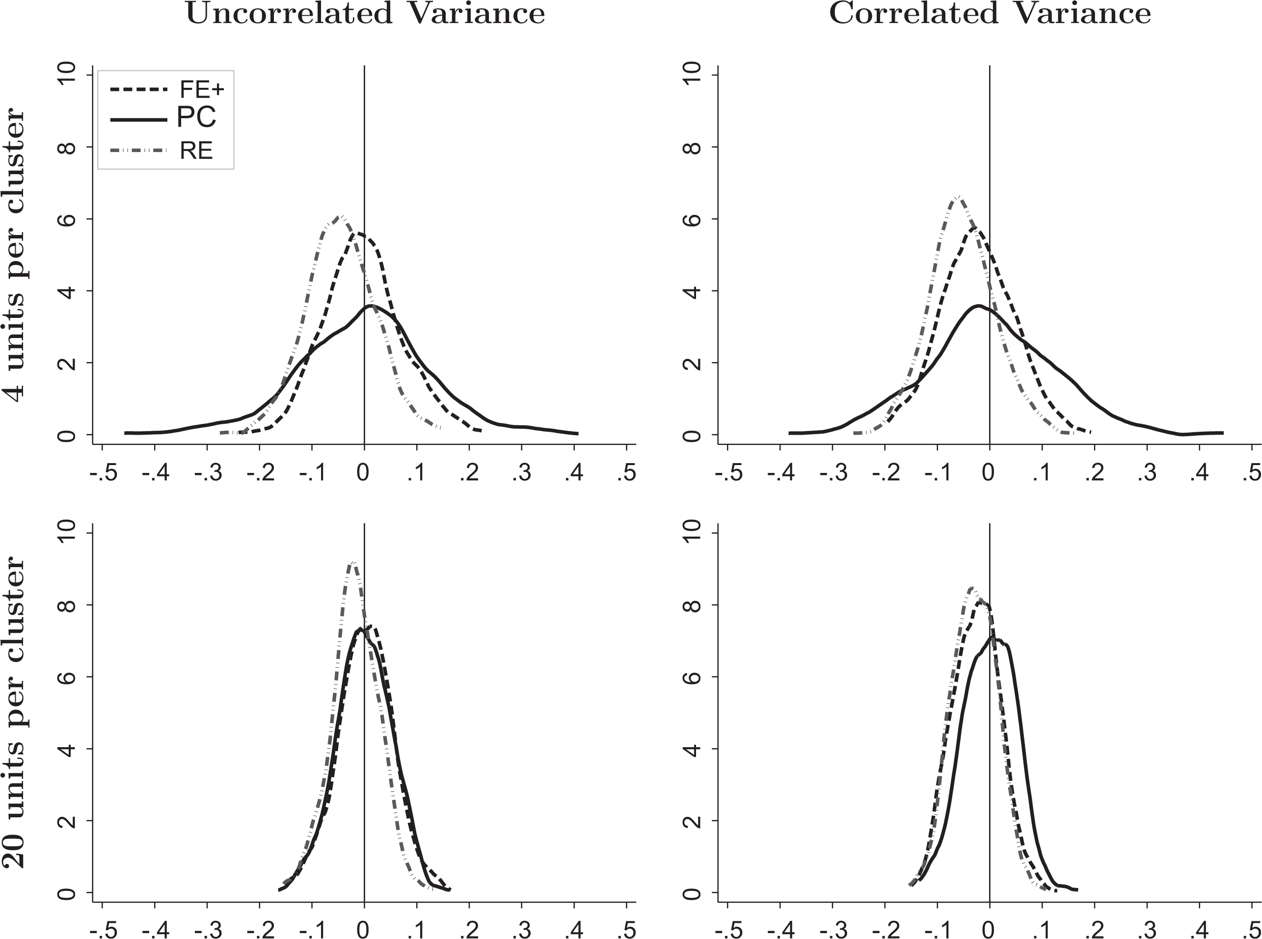
Kernel density plots of estimation errors, $\hat{γ} - γ_{1}$ , for coefficient of w_j across replications for all methods when the uncorrelated variance assumption holds (left panels) and when it is violated (right panels). Note. FE+ = augmented fixed-effects; PC = per-cluster regression; RE = random effects.

Given that β₁ was most affected by the violation of the uncorrelated variance assumption, we further investigated the effect of cluster size on the estimates of this regression coefficient. Figure 3 gives the estimated bias for each estimator across cluster sizes of 4, 8, 14, 20, and 50. The PC (solid) curve hugs the y = 0 line. The FE+ and RE curves cross at n = 20: As cluster size increases, the RE estimator’s bias decreases (dot-dashed curve), whereas the FE+ estimator’s bias is not as affected by cluster size, shown by its dashed curve staying relatively constant across the range of cluster sizes. Thus, cluster size has a differential effect on the bias of the estimators. When using bias to evaluate the estimators, our simulation study provides strong evidence that our proposed PC estimator outperforms the other estimators.

Figure 3.

Estimated bias for coefficient β₁ of x_ij versus cluster size. Note. FE+ = augmented fixed effects; PC = per-cluster regression; RE = random effects.

6.2.2 Precision and RMSE

As is often the case, there is a trade-off between bias and precision, which depends in part on the size of the clusters. The rank ordering of the estimators by their standard deviation (SD) is approximately the same for the three regression coefficients with slight differences between the smaller and larger cluster size conditions. Accordingly, we discuss how the precision of the estimators depends on cluster size, without distinguishing among the coefficients.

For the smaller cluster sizes of n = 4, RE produces the estimates with the smallest variances, followed by FE+, and PC produces the most variable estimates. This is clearly illustrated by comparing the widths of the empirical distributions of errors in Figure 1 or 2 for each estimator: The RE curves are the narrowest and the PC curves are the widest. For instance, for n = 4 and when the uncorrelated variance assumption is violated, the SD of ${\hat{β}}_{1 P C}$ over 500 replications is about 0.266, whereas for RE, the SD is less than half that at about 0.114 (see Tables C.1–C.3 in Online Appendix C for all SD values).

For the larger cluster size of n = 20, RE always yields the smallest variances, but the variances are not much smaller than those for FE+ and PC, which tend to have about equal variances. For instance, for β₁, for the large clusters and uncorrelated variance condition shown in the lower, left-hand panel of Figure 1, it is difficult to discern any differences in the widths of the distributions. Indeed, the SD for RE, in this case, is about 0.078 and the SDs for both FE+ and PC are 0.080.

With regard to precision, RE consistently outperforms FE+ and PC for all the regression coefficients and across all the simulation conditions. However, given the trade-off between bias and precision, it is useful to evaluate the estimators with regard to their RMSEs, which take both bias and imprecision into account. Given that the estimates of β₁ are the most affected by the simulation conditions and that precision depends on cluster size, we consider the RMSEs as a function of the extended range of cluster sizes for β₁ in Figure 4. Just as with bias in Figure 3, Figure 4 shows that the FE+ and RE curves cross with RE outperforming FE+ as cluster size increases. This figure also shows that, for the smallest cluster size of 4, the RMSE for PC is large and similar to that of RE. However, with clusters of at least 8, the PC estimator outperforms both RE and FE+ with regard to RMSE, providing strong evidence in favor of the PC estimator.

Figure 4.

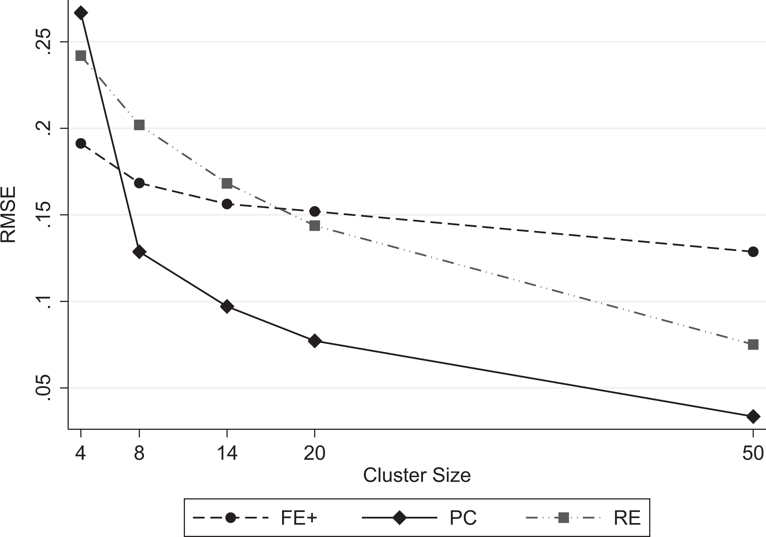
Estimated root mean square error (RMSE) for coefficient β₁ of x_ij versus cluster size. Note. FE+ = augmented fixed effects; PC = per-cluster regression; RE = random effects.

6.2.3 SE Estimation

As a final point, we evaluate the estimators in terms of how well their estimated SEs approximate the sampling SDs. We again focus on the most affected regression coefficient β₁. Figure 5 displays this ratio of mean SE to SD over the extended range of cluster sizes—similar to Figures 3 and 4. If the SE estimation works well, this ratio should equal 1. We see that both the PC (solid curve) and RE (dot-dashed curve) approaches provide good SE estimates. In contrast, for the FE+ approach, the SEs are increasingly underestimated as the cluster size increases. Although both the FE+ and PC approaches treat estimated coefficients from previous steps as known in the subsequent steps, it appears that underestimation of the SE is a larger problem for the FE+ approach. Accordingly, we recommend using either analytically derived or bootstrapped SEs for the FE+ approach. These could also be used for the PC approach and may be necessary if Step 1 is required.

Figure 5.

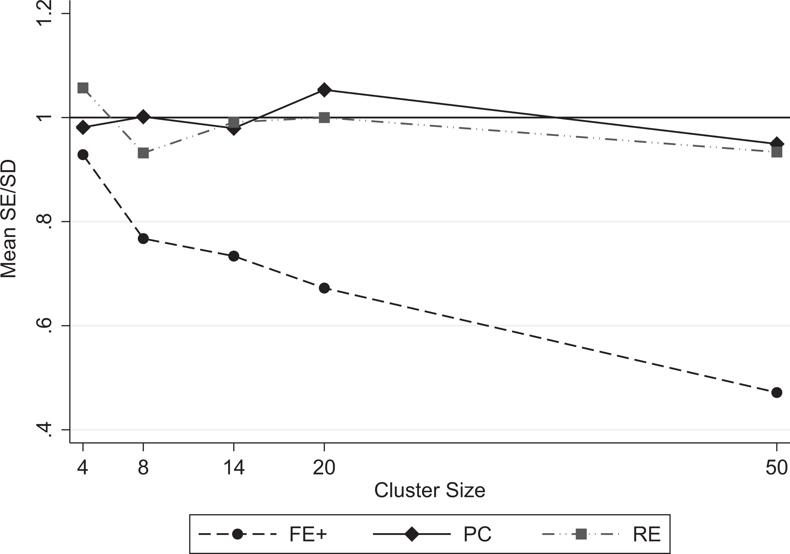
Ratio of mean standard errors (mean SEs) divided by standard deviations (SDs) of estimates versus cluster size. Note. FE+ = augmented fixed effects; PC = per-cluster regression; RE = random effects.

7 Conclusion

Given the popularity of multilevel models, studies that investigate potential biases for key parameters and provide simple solutions are clearly important. We have shown that commonly used random effects and FE estimators are biased in the presence of correlation between random effects and the within-cluster variance of unit-level covariates. Further, such bias can spill over to the estimation of coefficients of other covariates. We have proposed a new PC estimator that avoids such bias, produces good estimates of SEs, and generally has low RMSE. Consequently, we recommend broad use of PC when working with longitudinal or nested cross-sectional data when the clusters are sufficiently large. Stata code for applying this method to the HSB data is provided in Online Appendix B. In instances where the cluster sizes are small relative to the number of random effects, or where estimates for the random part of the model are of interest, we recommend using PC as part of a sensitivity analysis for alternative estimators.

Per-cluster methods have been used in the past for linear multilevel models (Burstein, Linn, & Capell, 1978, p. 369) and multilevel structural equation models (Chou, Bentler, & Pentz, 2000). Per-cluster methods can also be used for nonlinear multilevel models, such as probit models with random intercepts (Borjas & Sueyoshi, 1994) and logit models with random intercepts and slopes (Korn & Whittemore, 1979). However, the purpose of that work was to develop simple estimators and not to address endogeneity concerns. For our proposed PC estimator for linear models, it might appear to be inefficient to use OLS in the final step, not taking into account that the intercepts and slopes are estimated with different precision for different clusters. However, FGLS approaches, such as those discussed by Berkey, Hoaglin, Antczak-Bouckoms, Mosteller, and Golditz (1998), suffer from similar biases as RE estimators, as we confirmed in simulations (not shown).

An alternative approach for handling endogeneity, proposed for random-intercept models by Allison and Bollen (1997) and Teachman, Duncan, Yeung, and Levy (2001), is to model the unit-level covariates jointly with the responses using structural equation modeling and allow them to be correlated with the random intercept. This approach can be generalized to random-coefficient models but becomes infeasible for large cluster sizes.

In summary, we have demonstrated that our proposed, simple-to-implement PC approach outperforms standard estimators when estimating regression coefficients in multilevel models under violations of both the cluster-level exogeneity and uncorrelated variance assumptions. We recommend that researchers consider the validity of the uncorrelated variance assumption and add the PC method to their toolbox when investigating effects of covariates in cross-sectional and longitudinal analyses.

Footnotes

Declaration of Conflicting Interests

The author(s) declared no potential conflicts of interest with respect to the research, authorship, and/or publication of this article.

Funding

The author(s) disclosed receipt of the following financial support for the research, authorship, and/or publication of this article: The research reported here was supported by the Institute of Education Sciences, U.S. Department of Education, through grants R305B090011 to Michigan State University and R305B110017 to University of California, Berkeley. The opinions expressed are those of the authors and do not represent the views of the Institute or of the U.S. Department of Education.

Supplemental Material

The online appendices are available at .

References

Allison

P. D.

Bollen

K. A.

(1997). Change score, fixed effects, and random component models: A structural equation approach. Paper presented at the Annual Meeting of the American Sociological Association.

Ballou

Sanders

Wright

(2004). Controlling for student background variables in value-added assessment of teachers. Journal of Educational and Behavioral Statistics, 29, 37–65.

Berkey

C. S.

Hoaglin

D. C.

Antczak-Bouckoms

Mosteller

Golditz

G. A.

(1998). Meta-analysis of multiple outcomes by regression with random effects. Statistics in Medicine, 17, 2537–2550.

Borjas

G. J.

Sueyoshi

G. T.

(1994). A two-stage estimator for probit models with structural group effects. Journal of Econometrics, 64, 165–182.

Burstein

Linn

R. L.

Capell

F. J.

(1978). Analyzing multilevel data in the presence of heterogeneous within-class regressions. Journal of Educational Statistics, 3, 347–383.

Castellano

K. E.

Rabe-Hesketh

Skrondal

(2014). Composition, context, and endogeneity in school and teacher comparisons. Journal of Educational and Behavioral Statistics, 39, 333–367.

Chou

C.-P.

Bentler

P. M.

Pentz

M. A.

(2000). Two-stage approach to multilevel structural equation models: Application to longitudinal data. In Little

T. D.

Schnabel

K. U.

Baumert

(Eds.), Modeling longitudinal and multilevel data: Practical issues, applied approaches, and specific examples (pp. 33–49). Mahwah, NJ: Lawrence Erlbaum.

Chung

Gelman

Rabe-Hesketh

Liu

Dorie

(In press). Weakly informative prior for point estimation of covariance matrices in hierarchical models. Journal of Educational and Behavioral Statistics.

Don

Magnus

(1980). On the unbiasedness of iterated GLS estimators. Communications in Statistics—Theory and Methods, 9, 519–527.

10.

Frees

E. W.

(2004). Longitudinal and panel data: Analysis and applications for the social sciences. Cambridge, United Kingdom: Cambridge University Press.

11.

Hausman

J. A.

Taylor

W. E.

(1981). Panel data and unobservable individual effects. Econometrica, 49, 1377–1398.

12.

Kakwani

N. C.

(1967). The unbiasedness of Zellner’s seemingly unrelated regression equations estimators. Journal of the American Statistical Association, 62, 141–142.

13.

Kim

J. S.

Frees

E. W.

(2007). Multilevel modeling with correlated effects. Psychometrika, 72, 505–533.

14.

Korn

E. L.

Whittemore

A. S.

(1979). Methods for analyzing panel studies of acute health effects of air pollution. Biometrics, 35, 795–802.

15.

Mundlak

(1978). On the pooling of time series and cross-sectional data. Econometrica, 46, 69–86.

16.

Raudenbush

S. W.

Bryk

A. S.

(2002). Hierarchical linear models: Applications and data analysis methods (2nd ed.). Thousand Oaks, CA: Sage.

17.

Raudenbush

S. W.

Willms

J. D.

(1995). The estimation of school effects. Journal of Educational and Behavioral Statistics, 20, 307–335.

18.

Spanos

(2006). Where do statistical models come from? Revisiting the problem of specification. IMS Lecture Notes—Monograph Series 2nd Lehmann Symposium—Optimality, 49, 98–119.

19.

StataCorp. (2013). Stata: Statistics/data analysis [computer software]. College Station, TX: Author.

20.

Teachman

Duncan

G. J.

Yeung

W. J.

Levy

(2001). Covariance structure models for fixed and random effects. Sociological Methods & Research, 30, 271–288.

21.

Verbeke

Spiessens

Lesaffre

(2001). Conditional linear mixed models. American Statistician, 55, 25–34.

22.

Wiley

D. E.

(1975). Another hour, another day: Quantity for schooling, a potent path for policy. In Hauser

R. M.

Sewell

W. H.

Alwin

(Eds.), Schooling and achievement in American Society (pp. 225–265). New York, NY: Academic Press.

23.

Wooldridge

J. M.

(2005). Fixed-effects and related estimators for correlated random-coefficient and treatment-effect panel data models. Review of Economics and Statistics, 51, 385–390.

24.

Wooldridge

J. M.

(2010). Econometric analysis of cross-section and panel data. Cambridge, MA: The MIT Press.

Supplementary Material

Please find the following supplemental material available below.

For Open Access articles published under a Creative Commons License, all supplemental material carries the same license as the article it is associated with.

For non-Open Access articles published, all supplemental material carries a non-exclusive license, and permission requests for re-use of supplemental material or any part of supplemental material shall be sent directly to the copyright owner as specified in the copyright notice associated with the article.

0.00 MB

0.27 MB