An Evaluation of Empirical Bayes’s Estimation of Value-Added Teacher Performance Measures

Abstract

Empirical Bayes’s (EB) estimation has become a popular procedure used to calculate teacher value added, often as a way to make imprecise estimates more reliable. In this article, we review the theory of EB estimation and use simulated and real student achievement data to study the ability of EB estimators to properly rank teachers. We compare the performance of EB estimators with that of other widely used value-added estimators under different teacher assignment scenarios. We find that, although EB estimators generally perform well under random assignment (RA) of teachers to classrooms, their performance suffers under nonrandom teacher assignment. Under non-RA, estimators that explicitly (if imperfectly) control for the teacher assignment mechanism perform the best out of all the estimators we examine. We also find that shrinking the estimates, as in EB estimation, does not itself substantially boost performance.

Keywords

empirical Bayes’s estimation best linear unbiased predictor nonrandom assignment shrinkage estimators value-added measures

1. Introduction

Empirical Bayes’s (EB) estimation of teacher effects has gained recent popularity in the value-added research community (see, e.g., Chetty, Friedman, & Rockoff, 2014; Corcoran, Jennings, & Beveridge, 2011; Jacob & Lefgren, 2005, 2008; Kane & Staiger, 2008; and McCaffrey et al., 2004). Researchers motivate the use of EB estimation as a way to decrease classification error of teachers, especially when limited data are available to compute value-added estimates. Since teacher value-added estimates can be very noisy when there are only a small number of students per teacher, EB estimates of teacher value added reduce the variability of the estimates by shrinking them toward the average estimated teacher effect in the sample. As the degree of shrinkage depends on class size, estimates for teachers with smaller class sizes are more affected, potentially helping with the misclassification of these teachers. EB, or “shrinkage,” estimation may also be less computationally demanding than methods that view the teacher effects as fixed parameters to estimate. Finally, EB estimation has been motivated as a way to estimate teacher value added when including controls for peer effects and other classroom-level covariates.

This article analyzes the performance of EB estimation using both simulated and real student achievement data. We first provide a detailed theoretical derivation of the EB estimator, which has not previously been explicitly derived in the context of teacher value added. This theoretical discussion provides the basis for our expectations about how EB and other value-added estimators will perform under the different simulation scenarios we examine. We test our theoretical predictions by comparing the performance of EB estimators to estimators that treat the teacher effect as fixed. We first use a simulation, where the true teacher effect is known, comparing performance under random teacher assignment and various nonrandom assignment (non-RA) scenarios. In addition to the random versus fixed teacher effects comparison, we also examine whether shrinking the estimates improves performance. Finally, we apply these estimators to real student achievement data to see how the rankings of teachers vary across these estimators in a real-world setting.

Despite the potential benefits of EB estimation, we find that the estimated teacher effects can suffer from severe bias under nonrandom teacher assignment. By treating the teacher effects as random, EB estimation assumes that teacher assignment is uncorrelated with factors that predict student achievement—including observed factors such as past test scores. While the bias (technically, the inconsistency) disappears as the number of students per teacher increases—because the EB estimates converge to the so-called fixed effects (FE) estimates—the bias still can be important with the type of data used to estimate teacher value-added measures (VAMs). This is because the EB estimators of the coefficients on the covariates in the model are inconsistent for fixed class sizes as the number of classrooms grows. By contrast, estimators that include the teacher assignment indicators along with the covariates in a multiple regression analysis are consistent (as the number of classrooms grows) for the coefficients on the covariates. This generally leads to less bias in the estimated teacher VAMs under non-RA without many students per teacher.

The article begins in Section 2 with a detailed theoretical derivation of the EB estimator. Section 3 follows with a description of the five estimators we examine. Section 4 describes our simulation design and the different student grouping and teacher assignment scenarios we examine, with Section 5 providing the results of this analysis. Section 6 provides an analysis of these estimators using real student achievement data, and Section 7 concludes.

2. EB Estimation

There are several ways to derive EB estimators of teacher value added. We adopt the so-called mixed estimation approach, as in Ballou, Sanders, and Wright (2004), because it is fairly straightforward and does not require delving into Bayesian estimation methods. Our focus is on estimating teacher effects grade by grade. Therefore, we assume either that we have a single cross section or multiple cohorts of students for each teacher. We do not include cohort effects. Multiple cohorts are allowed by pooling students across cohorts for each teacher.

Let y_i denote a measure of achievement for student i randomly drawn from the population. This measure could be a test score or a gain score (i.e., current minus lagged score). Suppose there are G teachers and the teacher effects are b_g , g = 1, …, G. In the mixed effects setting, the b_g are treated as random variables drawn from a population of teacher effects, as opposed to fixed population parameters. Viewing the b_g as random variables independent of other observable factors affecting test scores has consequences for the properties of EB estimators.

Typically VAMs are estimated while controlling for other factors, which we denote by a row vector x _i . These factors include prior test scores and, in some cases, student-level and/or classroom-level covariates. We treat the coefficients on these covariates as fixed population parameters. We can write a mixed effects linear model as:

y_{i} = x_{i} γ + z_{i} b + u_{i},

where z _i is a 1 × G row vector of teacher assignment dummies, b is the G × 1 vector of teacher effects, and u_i contains the unobserved student-specific effects. Because a student is assigned to one and only one teacher, z_i ₁ + z_i ₂ + … + z_iG = 1. Equation 1 is an example of a “mixed model” because it includes the usual fixed population parameters γ and the random coefficients b. Even if there are no covariates, x _i typically includes an intercept. If x _i γ is only a constant, so x _i γ = γ, then γ is the average teacher effect and we can then assume E(b) = 0. This means that b_g is the effect of teacher g, net of the overall mean teacher effect.

Equation 1 is written for a particular student i so that teacher assignment is determined by the vector z _i . A standard assumption is that, conditional on b—so for a given set of teachers available for assignment—Equation 1 represents a linear conditional mean:

E (y_{i} | x_{i}, z_{i}, b) = x_{i} γ + z_{i} b,

which follows from Equation 1 and

E (u_{i} | x_{i}, z_{i}, b) = 0.

An important implication of Equation 3 is that u_i is necessarily uncorrelated with z _i , so that teacher assignment is not systematically related to unobserved student characteristics once we have controlled the observed factors in x _i .

If we assume a sample of N students assigned to one of G teachers, we can write Equation 1 in matrix notation as:

y = X γ + Z b + u,

where y and u are N × 1, X is N × K, and Z is N × G. In order to obtain the best linear unbiased estimator (BLUE) of γ and the best linear unbiased predictor (BLUP) of b, we assume that the covariates and teacher assignments satisfy a strict exogeneity assumption:

E (u_{i} | X, Z, b) = 0, i = 1, . . ., N .

An implication of Equation 5 is that inputs and teacher assignment of other students do not affect the outcome of student i.

Given Equation 5, we can write the conditional expectation of y as:

E (y | X, Z, b) = X γ + Z b .

In the EB literature, a standard assumption is:

b i s i n d e p e n d e n t o f (X, Z),

in which case:

E (y | X, Z) = X γ + Z E (b | X, Z) = X γ = E (y | X),

because $E (b | X, Z) = E (b) = 0$ . Equation 7 has the implication that teacher assignment for student i does not depend on the quality of the teacher (as measured by the b_g ).

From an econometric perspective, the statement $E (y | X) = X γ$ means that γ can be estimated in an unbiased way by an ordinary least square (OLS) regression of:

y_{i} o n x_{i}, i = 1, . . ., N .

Consequently, we can estimate the effects of the covariates x _i using a regression that completely ignores teacher assignment. As a practical matter, this has a very important implication when viewed from a classical, fixed parameters model—we are assuming that teacher assignment is uncorrelated with the covariates x _i . Correlation between teacher assignment and covariates in x _i is a potential source of bias in EB (and related) estimators of the teacher effects.

Under Equations 5 and 7, the OLS estimator of γ is unbiased and consistent, but it is inefficient if we impose the standard classical linear model assumptions on u. In particular, if the error variance has the usual scalar structure:

V a r (u | X, Z, b) = V a r (u) = σ_{u}^{2} I_{N},

then

\begin{aligned} V a r (y | X, Z) = E [(Z b + u) (Z b + u)^{'} | X, Z] \\ = Z V a r (b) Z^{'} + V a r (u) = σ_{b}^{2} Z Z^{'} + σ_{u}^{2} I_{N}, \end{aligned}

where we also add the standard assumption that the elements of b are uncorrelated:

V a r (b) = σ_{b}^{2} I_{G},

and $σ_{b}^{2}$ is the variance of the teacher effects, b_g .

Under the assumption that $σ_{b}^{2}$ and $σ_{u}^{2}$ (or at least their ratio) are known, the BLUE of γ under the preceding assumptions is the generalized least squares (GLS) estimator:

γ^{*} = {[X^{'} {(σ_{b}^{2} Z Z^{'} + σ_{u}^{2} I_{N})}^{- 1} X]}^{- 1} X^{'} {(σ_{b}^{2} Z Z^{'} + σ_{u}^{2} I_{N})}^{- 1} y .

The N × N matrix $Z Z^{'}$ is a block diagonal matrix with G blocks, where block g is an N_g × N_g matrix of ones and N_g is the number of students taught by teacher g. The GLS estimator γ* is the well-known “random effects” (REs) estimator popular from panel data and cluster sample analysis. However, it is important to understand that the “REs” in this case are teacher effects, not student-specific effects. Also, like the OLS estimator from Equation 9, the GLS estimator γ* does not partial out the teacher assignment.

Before we discuss γ* further, it is helpful to write down the mixed effects model in perhaps a more common form. After students have been designated to classrooms, we can write y_gi as the outcome for student i in class g and similarly for x _gi and u_gi . Then, for classroom g, we have:

y_{g i} = x_{g i} γ + b_{g} + u_{g i} \equiv x_{g i} γ + r_{g i}, i = 1, . . ., N_{g},

where r_gi ≡ b_g + u_gi is the composite error term. In other words, the variation in y_gi not explained by x _gi is due to teacher and individual student effects, and both of these (b_g and u_gi ) are assumed to be independent of x _gi . Equation 13 also makes it easy to see that the BLUE of γ is the REs estimator. Further, the assumption $E (u_{g i} | X_{g}, b_{g}) = 0$ implies that covariates from student h do not affect the outcome of student i. We can also see that OLS pooled across i and g is unbiased for γ because we are assuming $E (b_{g} | X_{g}) = 0$ .

What about estimation of b, the teacher effects? As shown in, say, Ballou et al. (2004), the BLUP of b under Assumptions 5, 7, and 10 is:

b^{*} = {(Z^{'} Z + ρ I_{G})}^{- 1} Z^{'} (y - X γ^{*}) \equiv {(Z^{'} Z + ρ I_{G})}^{- 1} {Z^{'} r}^{*},

where $ρ = σ_{u}^{2} / σ_{b}^{2}$ , and $r^{*} = y - X γ^{*}$ is the vector of residuals. Straightforward matrix algebra shows each $b_{g}^{*}$ can be expressed as:

\begin{aligned} b_{g}^{*} = {(N_{g} + ρ)}^{- 1} \sum_{i = 1}^{N_{g}} r_{g i}^{*} = (\frac{N_{g}}{N_{g} + ρ}) {\overset{ˉ}{r}}_{g}^{*} \\ = (\frac{σ_{b}^{2}}{σ_{b}^{2} + (σ_{u}^{2} / N_{g})}) {\overset{ˉ}{r}}_{g}^{*} = (\frac{σ_{b}^{2}}{σ_{b}^{2} + (σ_{u}^{2} / N_{g})}) ({\overset{ˉ}{y}}_{g} - {\overset{ˉ}{x}}_{g} γ^{*}), \end{aligned}

where:

{\overset{ˉ}{r}}_{g}^{*} = N_{g}^{- 1} \sum_{i = 1}^{N_{g}} r_{g i}^{*} = {\overset{ˉ}{y}}_{g} - {\overset{ˉ}{x}}_{g} γ^{*},

is the average of the residuals $r_{g i}^{*} = y_{g i} - x_{g i} γ^{*}$ within classroom g.

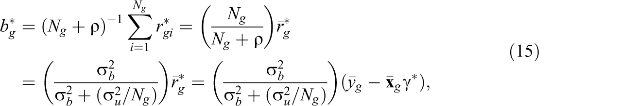
To operationalize γ* and $b_{g}^{*}$ , we must replace $σ_{b}^{2}$ and $σ_{u}^{2}$ with estimates. There are different ways to obtain estimates depending on whether one uses OLS residuals after an initial estimation or a joint estimation method. With the composite error defined as $r_{g i} = b_{g} + u_{g i}$ , we can write $σ_{r}^{2} = σ_{b}^{2} + σ_{u}^{2}$ . An estimator of $σ_{r}^{2}$ can be obtained from the usual sum of squared residuals from the OLS regression:

y_{g i} o n x_{g i}, i = 1, . . ., N_{g}, g = 1, . . ., G .

Call the residuals ${\tilde{r}}_{g i}$ . Then a consistent estimator is:

{\tilde{σ}}_{r}^{2} = \frac{1}{(N - K)} \sum_{g = 1}^{G} \sum_{i = 1}^{N_{g}} {\tilde{r}}_{g i}^{2},

which is just the usual degrees-of-freedom (df) adjusted error variance estimator from OLS.

To estimate $σ_{u}^{2}$ , write $r_{g i} - {\overset{ˉ}{r}}_{g} = u_{g i} - {\overset{ˉ}{u}}_{g}$ , where ${\overset{ˉ}{r}}_{g}$ is the within-teacher average, and similarly for ${\overset{ˉ}{u}}_{g}$ . A standard result on demeaning a set of uncorrelated random variables with the same variance gives $V a r (u_{g i} - {\overset{ˉ}{u}}_{g}) = σ_{u}^{2} (1 - N_{g}^{- 1})$ and so, for each g, $E [\sum_{i = 1}^{N_{g}} {(r_{g i} - {\overset{ˉ}{r}}_{g})}^{2}] = σ_{u}^{2} (N_{g} - 1) .$ When we sum across teachers it follows that:

\frac{1}{(N - G)} \sum_{g = 1}^{G} \sum_{i = 1}^{N_{g}} {(r_{g i} - {\overset{ˉ}{r}}_{g})}^{2},

has expected value $σ_{u}^{2}$ . To turn Equation 19 into an estimator, we can replace r_gi with the OLS residuals, ${\tilde{r}}_{g i}$ , from the regression in Equation 17. The estimator based on the OLS residuals is:

{\tilde{σ}}_{u}^{2} = \frac{1}{(N - G)} \sum_{g = 1}^{G} \sum_{i = 1}^{N_{g}} {({\tilde{r}}_{g i} - {\overline{\tilde{r}}}_{g})}^{2} .

With fixed class sizes and G getting large, the estimator that uses N in place of N − G is not consistent. Therefore, we prefer the estimator in Equation 20, as it should have less bias in applications where G/N is not small. With many students per teacher, the difference should be minor. We could also use N – G − K as a further df adjustment but subtracting off K does not affect the consistency.

Given ${\tilde{σ}}_{r}^{2}$ and ${\tilde{σ}}_{u}^{2}$ , we can estimate $σ_{b}^{2}$ as:

{\tilde{σ}}_{b}^{2} = {\tilde{σ}}_{r}^{2} - {\tilde{σ}}_{u}^{2} .

In any particular data set—especially if the data have been generated to violate the standard assumptions listed previously—there is no guarantee that Equation 21 is nonnegative. A simple solution to this problem (and one used in software packages, such as Stata) is to set ${\tilde{σ}}_{b}^{2} = 0$ whenever ${\tilde{σ}}_{r}^{2} < {\tilde{σ}}_{u}^{2}$ . In order to ensure this happens infrequently with multiple cohorts, we compute ${\tilde{σ}}_{u}^{2}$ by replacing ${\overline{\tilde{r}}}_{g}$ with the average obtained for the particular cohort. This ensures that, for a given cohort, the terms $\sum_{i = 1}^{N_{g}} {({\tilde{r}}_{g i} - {\overline{\tilde{r}}}_{g})}^{2}$ are as small as possible. In theory, if there are no cohort effects, we could use an overall cohort mean for ${\overline{\tilde{r}}}_{g}$ . But using cohort-specific means reduces the problem of negative ${\tilde{σ}}_{b}^{2}$ when the model is misspecified.

An appealing alternative is to estimate $σ_{b}^{2}$ and $σ_{u}^{2}$ jointly along with γ, using software that ensures nonnegativity of the variance estimates. The most common approach to doing so is to assume joint normality of the teacher effects, b_g , and the student effects, u_gi , across all g and i—along with the previous assumptions. One important point is that the resulting estimators are consistent even without the normality assumption; so, technically, we can think of them as “quasi-” maximum likelihood estimators (MLEs). The MLE of $σ_{u}^{2}$ has the same form as in Equation 20, except the residuals are based on the MLE of γ rather than the OLS estimator. A similar comment holds for the MLE of $σ_{b}^{2}$ (if we do not constrain it to be nonnegative). See, for example, Hsiao (2003, section 3.3.3).

Unlike the GLS estimator of γ, the feasible GLS (FGLS) estimator is no longer unbiased (even under Equations 5 and 7), and so we must rely on asymptotic theory. In the current context, the estimator is known to be consistent and asymptotically normal provided $G \to \infty$ with N_g fixed. In simulations, Hansen (2007) shows that the asymptotic properties work well when G is roughly around 40 with N_g of a similar magnitude, and even somewhat larger. Consequently, the asymtptotic approximations for the FGLS estimator of γ should be reliable in the vast majority of VAM applications, which are typically applied at the district or state level with a large number of teachers. In any case, our focus in this article is not on estimation of γ but rather the teacher effects, b. Often we can estimate b well, at least for ranking purposes, even when our estimator of g is severely biased. For estimating b, the number of students per teacher is what matters most. In fact, without x _i in the equation, it is only the number of students per teacher that matters. In our simulations, we use relatively few teachers (age 36), because adding more teachers does not change our ability to estimate the effects for a particular teacher.

When γ* is replaced with the FGLS estimator and the variances $σ_{b}^{2}$ and $σ_{u}^{2}$ are replaced with estimators, the EB estimator of b is no longer a BLUP. Nevertheless, we use the same formula as in Equation 15 for operationalizing the BLUPs. Conveniently, certain statistical packages—such as Stata 12 with its “xtmixed” command—allow one to recover the operationalized BLUPs after MLE. When we use the (quasi-)MLEs to obtain $b_{g}^{*}$ , we obtain what are typically called the EB estimates.

One way to understand the shrinkage nature of $b_{g}^{*}$ is to compare it with the estimator obtained by treating the teacher effects as fixed parameters. Let $\hat{γ}$ and $\hat{β}$ be the OLS estimators from the regression:

y_{i} o n x_{i}, z_{i}, i = 1, . . ., N .

Then $\hat{γ}$ is the so-called FE estimator obtained by a regression of y_i on the controls in x _i and the teacher assignment dummies in z _i . As with the “REs” terminology, it is important to understand that regression in Equation 22 incorporates teacher FE, not student FE. In the context of the classical fixed parameters model:

y = X γ + Z β + u,

E (u | X, Z) = 0, V a r (u | X, Z) = σ_{u}^{2} I_{N},

$\hat{γ}$ is the BLUE of γ and $\hat{β}$ is the BLUE of β. As is well known, $\hat{γ}$ can be obtained by an OLS regression where y_gi and x _gi have been deviated from within-teacher averages (see, e.g., Wooldridge, 2010, chapter 10). Further, the estimated teacher FE can be obtained as:

{\hat{β}}_{g} = {\overset{ˉ}{y}}_{g} - {\overset{ˉ}{x}}_{g} \hat{γ} .

Equation 24 makes computation of the teacher VAMs efficient if one does not want to run the long regression in Equation 22.

By comparing Equations 15 and 24, we see that the EB estimator $b_{g}^{*}$ differs from the FE estimator ${\hat{β}}_{g}$ in two ways. First, and most importantly, the RE estimator $γ^{*}$ is used in computing $b_{g}^{*}$ , while ${\hat{β}}_{g}$ uses the FE estimator $\hat{γ}$ . Second, $b_{g}^{*}$ shrinks the average of the residuals toward zero by the factor:

\frac{σ_{b}^{2}}{σ_{b}^{2} + (σ_{u}^{2} / N_{g})} = \frac{1}{1 + (ρ / N_{g})},

where:

ρ = σ_{u}^{2} / σ_{b}^{2} .

Equation 25 illustrates the well-known result that the smaller the number of students taught by teacher g, N_g , the more the average residual (AR) is shrunk toward zero.

A well-known algebraic result—for example, Wooldridge (2010, chapter 10)—that holds for any given number of teachers G is that:

γ^{*} \to \hat{γ} a s ρ \to 0 o r N_{g} \to \infty .

Equation 27 can be verified¹ by noting that the RE estimator of γ can be obtained from the pooled OLS regression:

y_{g i} - θ_{g} {\overset{ˉ}{y}}_{g} o n x_{g i} - θ_{g} {\overset{ˉ}{x}}_{g},

where:

θ_{g} = 1 - {(\frac{σ_{u}^{2}}{σ_{u}^{2} + N_{g} σ_{b}^{2}})}^{1 / 2} = 1 - {(\frac{1}{1 + (N_{g} / ρ)})}^{1 / 2} .

It is easily seen that $θ_{g} \to 1$ as $ρ \to 0$ or $N_{g} \to \infty$ . In other words, with many students per teacher or a large teacher effect variance relative to the student effect variance, the RE and FE estimates can be very close but never identical. Not coincidentally, the shrinkage factor in Equation 25 tends to unity if $ρ \to 0$ or $N_{g} \to \infty$ . The bottom line is that with a “large” number of students per teacher, the shrinkage estimates of the teacher effects can be close to the FE estimates. The RE and FE estimates also tend to be similar when $σ_{u}^{2}$ (the student effect) is “small” relative to $σ_{b}^{2}$ (the teacher effect) but is an unlikely scenario.

An important point that appears to go unnoticed in applying the shrinkage approach is that, in situations where γ* and $\hat{γ}$ substantively differ, γ* suffers from systematic bias because it assumes teacher assignment is uncorrelated with x _i . Because γ* is used in constructing the $b_{g}^{*}$ in Equation 15, the bias in γ* generally results in biased teacher effects, which would be biased even if Equation 15 did not employ a shrinkage factor. The shrinkage likely exacerbates the problem, that is, the estimates are being shrunk toward values that are systematically biased for the teacher effects.²

The expressions in Equations 15 and 24 motivate a common two-step alternative to the EB and FE approaches. In the first step of the procedure, one obtains $\tilde{γ}$ using the OLS regression in Equation 17 and obtains the residuals, ${\tilde{r}}_{g i}$ . In the second step, one averages the residuals ${\tilde{r}}_{g i}$ within each teacher to obtain the teacher effect for teacher g. These estimated teacher effects can be expressed as:

{\tilde{β}}_{g} = N_{g}^{- 1} \sum_{i = 1}^{N_{g}} {\tilde{r}}_{g i} = {\overset{ˉ}{y}}_{g} - {\overset{ˉ}{x}}_{g} \tilde{γ},

which has the same form as Equation 24 with the important difference that $\tilde{γ}$ is used in place of $\hat{γ}$ . We call this approach the AR method. After obtaining the averages of the residuals one can, in a third step, shrink the averages using the EB shrinkage factors in Equation 15. This “shrunken AR” (SAR) method typically obtains the shrinkage factors using the estimates in Equations 18 and 20.

With or without shrinking, the AR approach suffers from systematic bias if teacher assignment, z _i , is correlated with the covariates, x _i . In effect, the AR approach partials x _i out of y_i but does not partial x _i out of z _i , the latter of which is crucial if x _i and z _i are correlated. The so-called FE regression in Equation 22 partials x _i out of z _i , which makes it a more reliable estimator under nonrandom teacher assignment—perhaps much more reliable with strong forms of non-RA. Since the FE estimation of the teacher VAMs allows any correlation between z _i and x _i , we thus expect it to outperform EB estimation and strongly outperform SAR under non-RA. The bias due to nonrandom allocation of students to teachers is also discussed in Rothstein (2009, 2010).

It is also important to know that the SAR approach is inferior to the EB approach under non-RA. The logic is simple. First, the algebraic relationship between RE and FE means that γ* tends to be closer to the FE estimator, $\hat{γ}$ , than the OLS estimator, $\tilde{γ}$ . Consequently, under nonrandom teacher assignment, the estimated teacher effects using the RE estimator of γ will have less bias than the estimates that begin with OLS estimation of γ. Second, if teacher assignment is uncorrelated with the covariates, the OLS estimator of γ is inefficient relative to the RE estimator under the standard REs assumptions (because the RE estimator is FGLS). Thus, the only possible justification for SAR is computational simplicity when the number of controls in x _i is very large. For the kinds of data sets widely available, the computational saving from using SAR rather than EB is likely to be minor.

3. Summary of Estimation Methods

In this article, we examine five different value-added estimators used to recover the teacher effects and apply them to both real and simulated data. Some of the estimators use EB or shrinkage techniques, while others do not. They can all be cast as a special case of the estimators described in the previous section. For clarity, we briefly describe each one, with additional reference to each of these specifications provided in Table A1. Associated Stata 12 code is available upon request.

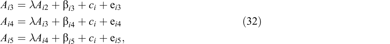
The estimators can be obtained from a dynamic equation of the form:

A_{i t} = λ A_{i, t - 1} + X_{i t} γ + Z_{i t} β + v_{i t},

in which A_it is achievement (measured by a test score) for student i in grade t, X _it is a vector of student characteristics, and Z _it is the vector of teacher assignment dummies. This is similar to Equation 1 but with the lagged test score written separately from X _it for clarity. Also, X _it is omitted from the estimation of the teacher effects in the simulation analysis mentioned subsequently, as student characteristics are not included in the data generating process. The EB estimator we analyzed in Section 2 was for the case of a single cross section of students, and so we only use one grade—fifth grade—for the analysis.

We first analyze EB LAG, a dynamic MLE version of the EB estimator that treats the teacher effects as random. This technique obtains the estimates of the teacher effects using the normal maximum likelihood in the first stage, where the error includes teacher REs (along with the student-specific error). In the second stage, the shrinkage factor is applied to these teacher effects. As described in Rabe-Hesketh and Skrondal (2012), this two-step procedure can be performed in one step using the “xtmixed” command in Stata 12 with teacher REs. The predicted REs of this regression are identical to shrinking the MLE estimates by the shrinkage factor. This procedure is generally justified even if the unobservables do not have normal distributions, in which case we are applying quasi-MLE. A second estimator we consider is the AR method described in Section 2, which is obtained by first using the OLS regression in Equation 17 and then using Equation 30. Recall that the AR method essentially differs from EB LAG in that it uses OLS to estimate γ in the first stage.³ We expect the EB LAG estimator to outperform the AR estimator in most scenarios, given that EB LAG generally uses a more reliable estimator of γ.

We compare the AR and EB estimators with estimators that partial out teacher assignment when estimating γ, thereby allowing teacher assignments that are correlated with lagged test scores and student characteristics. This third estimator is obtained by simply applying OLS to Equation 31, by pooling across students and classrooms. We call this the “dynamic OLS” or “DOLS” estimator. The inclusion of the lagged test score accounts for the possibility that teacher assignment is related to students’ most recent test score. Guarino, Reckase, and Wooldridge (2015) discuss the assumptions under which DOLS consistently estimates β when Equation 31 is obtained from a structural cumulative effects model, and the assumptions are quite restrictive. More importantly, their simulations show the DOLS estimator often estimates β well, at least for ranking purposes, even when the assumptions underlying the consistency of DOLS fail.

Given that EB estimation is often motivated as a way to increase precision and decrease misclassification, we also analyze whether shrinking AR and DOLS estimates enhances performance. Thus, the fourth estimator we analyze is our SAR estimator. This estimator takes the AR estimates from Equation 17 and shrinks them by the shrinkage factor described in Equation 25. Shrinking the AR estimates does not result in a true EB estimator since AR uses OLS in the first stage, but it is commonly used as a simpler way of operationalizing the EB approach (see, e.g., Kane & Staiger, 2008). As discussed in Section 2, with a sufficiently large number of students per teacher, the EB LAG estimator converges to the DOLS estimator, but SAR does not. Thus, as the number of students per teacher grows, we would expect EB LAG to perform more similarly to DOLS than SAR. Finally, we consider a shrunken DOLS (SDOLS) estimator, which takes the DOLS estimated teacher FE and shrinks them by the shrinkage factor derived in Section 2. Although SDOLS is rarely done in practice and is not a true EB estimator, we include it as an exploratory exercise in order to better determine the effects of shrinking itself when the number of students per teacher differs. When the class sizes are all the same, the shrunken estimates (SDOLS and SAR) will only differ from the unshrunken estimates by a constant positive multiple. Thus, shrinking the DOLS or AR estimates will have no effect in terms of ranking teachers. It is important to keep in mind that, unlike DOLS and SDOLS, the AR and SAR estimators do not allow for general correlation between the teacher assignment and past test scores (or other covariates).

4. Comparing VAM Methods Using Simulated Data

The question of which VAM estimators perform the best can only be addressed in simulations where the true teacher effects are known. Therefore, to evaluate the performance of EB estimators relative to other common value-added estimators, we apply these methods to simulated data. This approach allows us to examine how well various estimators recover the true teacher effects under a variety of student grouping and teacher assignment scenarios. Using data generated as described in Section 4.1, we apply the value-added estimators discussed in Section 3 and compare the resulting estimates with the true teacher effects.

4.1. Simulation Design

Much of our main analysis focuses on a base case that restricts the data generating process to a relatively narrow set of idealized conditions (e.g., no measurement error and no peer effects, constant teacher effects). However, we do relax some of these conditions as sensitivity tests of the main results. The data are constructed to represent Grades 3 through 5 (the tested grades) in a hypothetical school. For simplicity and comparison with the theoretical predictions, we assume that the learning process has been going on for a few years but only calculate estimates of teacher effects for fifth-grade teachers—a single cross section.⁴ We create data sets that contain students nested within teachers, with students followed longitudinally over time in order to reflect the institutional structure of an elementary school. Our simple baseline data generating process is as follows:

\begin{aligned} A_{i 3} = λ A_{i 2} + β_{i 3} + c_{i} + e_{i 3} \\ A_{i 4} = λ A_{i 3} + β_{i 4} + c_{i} + e_{i 4} \\ A_{i 5} = λ A_{i 4} + β_{i 5} + c_{i} + e_{i 5}, \end{aligned}

in which A_i ₂ is a baseline score reflecting the subject-specific knowledge of child i entering third grade; A_it is the grade − t test score (t = 3, 4, 5); λ is a time constant decay parameter, where λ is set equal to zero in the simulations for lag scores greater than 1 year prior; β _it is the teacher-specific contribution to growth (the true teacher value-added effect); c_i is a time-invariant student-specific effect (may be thought of as “ability” or “motivation”); and e _it is a random deviation for each student. We assume independence of e _it over time, a restriction implying that past shocks to student learning decay at the same rate as all inputs (see Guarino, Reckase, & Wooldridge, 2015, for a more detailed discussion of this “common factor restriction” assumption). In all of the simulations reported in this article, the random variables A_i ₂, β _it , c_i , and e _it are drawn from normal distributions with zero means. The standard deviation of the teacher effect is .25, the standard deviation of the student fixed effect is .5, and the standard deviation of the random noise component is 1. These give relative shares of 5%, 19%, and 76% of the total variance in gain scores (when λ = 1), respectively. Given that the student and noise components are larger than the teacher effects, we call these “small” teacher effects. We also conduct a sensitivity analysis using “large” teacher effects, where the true teacher effects are drawn from a distribution with a standard deviation of 1. The baseline score is drawn from a distribution with a standard deviation of 1. We also allow for correlation between the time-invariant child-specific heterogeneity, c_i , and the baseline test score, A_i ₂, which we set to $0.5$ . This correlation reflects that students with better unobserved “ability” likely have higher test scores as well.

Our data are simulated using 36 teachers per grade and 720 students per cohort. For estimating teacher effects, it is the number of student per teacher that is important. The number of teachers only impacts the precision of the estimates of λ and the population variances and, as discussed earlier, results in Hansen (2007) indicate that 36 teachers is sufficient. In order to create a situation in which there is a substantial variation in class size—to showcase the potential disparities between EB/shrinkage and other estimators—we vary the number of students per classroom. Teachers receive classes of varying sizes but receive the same number of students in each cohort. The size of class each teacher receives is random but ensures that 12 teachers have classes of 10 students, 12 teachers have a class size of 20, and 12 teachers have class sizes of 30. We simulate the data using both one and four cohorts of students to provide further variation in the amount of data from which the teacher effects are calculated. In the case of four cohorts, data are pooled across the cohorts so that value-added estimates are based on sample sizes of 40, 80, and 120, instead of 10, 20, and 30 as in the one-cohort case. Therefore, we would expect that estimates in the four-cohort case to be less noisy than those from the one-cohort case, possibly mitigating the potential gains from EB estimation.

To create different scenarios, we vary two key features, namely, the grouping of students into classes and the assignment of classes of students to teachers within schools. We generate data using each of the seven different mechanisms for the assignment of students outlined in Table A2. Students are grouped into classrooms either randomly, based on their prior year achievement level (dynamic grouping [DG]), or based on their unobserved heterogeneity (heterogeneity grouping [HG]). In the random case, students are assigned a random number and then grouped into classrooms of various sizes based on that random number. In the grouping cases, students are ranked by either the prior test score or their fixed effect and grouped into classrooms of various sizes based on that ranking. Teachers are assigned to these classrooms either randomly (denoted RA) or nonrandomly. Teachers assigned nonrandomly can be assigned positively (denoted positive assignment [PA]), meaning the best teachers are assigned to classrooms with the best students, or negatively (denoted negative assignment [NA]), meaning the best teachers are assigned to classrooms with the worst students.

These grouping and assignment procedures are not purely deterministic, as we allow for a random component with standard deviation of 1 in the assignment mechanism. As a sensitivity analysis, we also set this standard deviation to 0.1, meaning the grouping of students into classrooms is more deterministic. We use the estimators discussed in Section 3, but with only a constant, teacher dummies (if applicable), and the lagged test score included as covariates. We use 100 Monte Carlo replications per scenario in evaluating each estimator.

4.2. Evaluation Measures

For each estimator across each iteration, we save the individual estimated teacher effects and also retain the true teacher effects, which are fixed across the iterations for each teacher. To study how well the methods recover the true teacher effects, we adopt five simple summary measures using the teacher-level data. The first is a measure of how well the estimates preserve the rankings of the true teacher effects. We compute the Spearman rank correlation, $\hat{ρ}$ , between the estimated teacher effects and the true effects and report the average $\hat{ρ}$ across the 100 iterations. Second, we compute a measure of misclassification. These misclassification rates are obtained as the percentage of above-average teachers in the true quality distribution (i.e., teachers with true β _g > 0), who are misclassified as below average in the distribution of estimated teacher effects for the given estimator. Given that this is just an arbitrary cutoff point, we also obtain the fraction of teachers in the outside tails of the distribution that are incorrectly classified (e.g., fraction of teachers that are in the bottom quintile of the true distribution but estimated to lie in one of the other four quintiles).

In addition to examining rank correlations and misclassification rates, it is also helpful to have a measure that quantifies some notion of the magnitude of the bias in the estimates. Given that some teacher effects are biased upward and others downward, it is difficult to capture the overall bias in the estimates in a simple way. For each simulation, we create a statistic, $\hat{θ}$ , that captures how closely the magnitude of the deviation of the estimates from their mean tracks the magnitude of the deviation of the true effects from the true mean. To calculate this measure, we regress the deviation of the estimated teacher effects from their overall estimated means on the analogous deviation of the true effects generated from the simulation—for each estimator. We can represent this simple regression as:

{\hat{β}}_{g} - \overset{ˉ}{\hat{β}} = \hat{θ} (β_{g} - \overset{ˉ}{β}) + {r e s i d u a l}_{g},

in which ${\hat{β}}_{g}$ is the estimated teacher effect and β _g is the true effect of teacher g. From this simple regression, we report the average coefficient, $\overset{ˉ}{\hat{θ}}$ , across the 100 replications of the simulation for each estimator. This regression tells us whether the estimated teacher effects are correctly distributed around the average teacher. If $\hat{θ} = 1$ , then a movement of β _g away from its mean is tracked by the same movement of ${\hat{β}}_{g}$ from its mean. Because the estimated teacher effects are deviated from the overall mean of the estimated effect, $\overset{ˉ}{\hat{θ}}$ will not pick up additive bias that affects each teacher effect in the same way. However, one is not typically concerned about such biases if the estimated effects are used for comparisons among teachers.

When $\hat{θ} \approx 1$ , it makes sense to compare the magnitudes of the estimated teacher effects across teachers. If $\hat{θ} > 1$ , the estimated teacher effects amplify the true teacher effects. In other words, teachers above average will be estimated to be even more above average and vice versa for below-average teachers. An estimation method that produces $\hat{θ}$ substantially above one generally does a good job of ranking teachers, but the magnitudes of the differences in estimated teacher effects cannot be trusted. The magnitudes also cannot be trusted if $\hat{θ} < 1$ , and ranking the teachers generally becomes more difficult since the estimated effects are compressed relative to the true teacher effects. In some policy applications, the relative magnitudes of the estimated teacher effects might be important, and so we report the average value of $\hat{θ}$ across the simulations. Doing so allows us to determine scenarios where the magnitudes of estimated teacher effects are meaningful. Further, the measure provides insight into why some methods rank teachers relatively well even when the estimated effects are systematically biased, often quite badly.

The precision of these methods is also a key consideration when evaluating the overall performance. As described in Section 2, EB methods are not unbiased when the teacher effects are treated as fixed parameters we are trying to estimate. However, if the identifying assumptions hold, these methods should provide more precise estimates. This is one motivation for using EB methods, as estimates should be more stable over time, leading to a smaller variance in the teacher effects. As the teacher effect is fixed for each teacher across the 100 iterations, we have 100 estimates of each teacher effect. As a summary measure for the precision of the estimators, we calculate the standard deviation of the 100 teacher effect estimates for each teacher and then take a simple average across all teachers.

Finally, to further analyze the variance-bias trade-off for each of these estimators, we also include the average mean squared error (MSE). This measure averages the following across all g teachers and across simulation runs:

\hat{M S E_{g}} = {(β_{g} - {\hat{β}}_{g})}^{2} .

This provides a simple statistic to determine whether the bias induced by shrinking is justifiable due to gains in precision.

5. Simulation Results

Tables 1 and 2 report the five evaluation measures described in Section 4.2 for each particular estimator-assignment scenario combination. For ease in interpreting the tables, a quick guide to the descriptions of each of these estimators, grouping-assignment mechanisms, and evaluation measures can be found in Appendix Tables A1 through A3. As these shrinkage and EB estimators are often motivated as a way to reduce noise, one might expect these approaches to be most beneficial with very limited student data per teacher. Thus, we estimate teacher effects using both four cohorts and one cohort of data. The tables show results for the case λ = .5. Although not reported, we also conducted a full set of simulations for λ = .75 and λ = 1, and the main conclusions are unchanged. The full set of simulation results is available upon request from the authors.

Table 1

Simulation Results: Comparing Fixed and Random Teacher Effects Estimators

λ = .5		Four Cohorts			One Cohort
G-A Mechanism	Evaluation Type	DOLS	AR	EB LAG	DOLS	AR	EB LAG
RA	Rank correlation	.85	.85	.86	.65	.65	.67
	Misclassification	.15	.15	.15	.25	.25	.26
	Average θ	1.01	1.01	0.78	1.03	1.03	0.49
	Average SD	0.13	0.14	0.12	0.28	0.27	0.18
	MSE	0.018	0.019	0.013	0.076	0.076	0.034
DG-RA	Rank correlation	.85	.85	.86	.64	.64	.65
	Misclassification	.15	.16	.16	.26	.25	.25
	Average θ	1.01	0.99	0.77	1.00	0.98	0.45
	Average SD	0.14	0.14	0.12	0.27	0.27	0.19
	MSE	0.019	0.020	0.014	0.075	0.071	0.034
DG-PA	Rank correlation	.86	.60	.76	.63	.38	.45
	Misclassification	.15	.28	.22	.26	.35	.48
	Average θ	0.99	0.53	0.49	0.98	0.52	0.16
	Average SD	0.13	0.19	0.16	0.27	0.30	0.22
	MSE	0.018	0.037	0.024	0.074	0.091	0.051
DG-NA	Rank correlation	.85	.62	.78	.67	.41	.48
	Misclassification	.14	.26	.20	.25	.34	.47
	Average θ	1.01	0.54	0.53	1.03	0.54	0.17
	Average SD	0.14	0.19	0.15	0.27	0.29	0.22
	MSE	0.019	0.035	0.022	0.074	0.086	0.050
HG-RA	Rank correlation	.72	.73	.73	.58	.59	.60
	Misclassification	.23	.22	.23	.29	.29	.30
	Average θ	1.02	1.02	0.86	1.00	0.99	0.54
	Average SD	0.21	0.21	0.18	0.32	0.31	0.21
	MSE	0.046	0.045	0.033	0.100	0.097	0.044
HG-PA	Rank correlation	.94	.93	.94	.81	.79	.81
	Misclassification	.09	.10	.10	.17	.18	.19
	Average θ	1.61	1.52	1.43	1.60	1.51	1.06
	Average SD	0.20	0.19	0.16	0.31	0.30	0.19
	MSE	0.042	0.038	0.027	0.097	0.092	0.035
HG-NA	Rank correlation	.39	.38	.41	.26	.25	.28
	Misclassification	.35	.35	.38	.40	.41	.55
	Average θ	0.33	0.32	0.15	0.34	0.33	0.06
	Average SD	0.22	0.23	0.22	0.32	0.32	0.24
	MSE	0.050	0.052	0.047	0.101	0.102	0.058

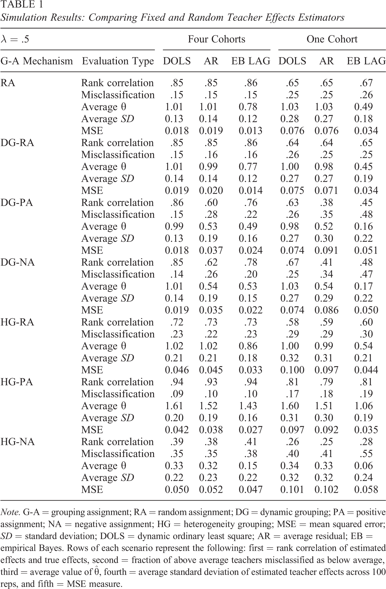
Note. G-A = grouping assignment; RA = random assignment; DG = dynamic grouping; PA = positive assignment; NA = negative assignment; HG = heterogeneity grouping; MSE = mean squared error; SD = standard deviation; DOLS = dynamic ordinary least square; AR = average residual; EB = empirical Bayes. Rows of each scenario represent the following: first = rank correlation of estimated effects and true effects, second = fraction of above average teachers misclassified as below average, third = average value of $\hat{θ}$ , fourth = average standard deviation of estimated teacher effects across 100 reps, and fifth = MSE measure.

Table 2

Simulation Results: Comparing Shrunken and Unshrunken Estimators

λ = .5		Four Cohorts				One Cohort
G-A Mechanism	Evaluation Type	DOLS	SDOLS	AR	SAR	DOLS	SDOLS	AR	SAR
RA	Rank correlation	.85	.85	.85	.85	.65	.66	.65	.66
	Misclassification	.15	.15	.15	.15	.25	.25	.25	.25
	Average θ	1.01	1.01	1.01	1.01	1.03	0.99	1.03	0.99
	Average SD	0.13	0.13	0.14	0.14	0.28	0.26	0.27	0.26
	MSE	0.018	0.018	0.019	0.019	0.076	0.068	0.076	0.068
DG-RA	Rank correlation	.85	.85	.85	.85	.64	.64	.64	.64
	Misclassification	.15	.15	.16	.16	.26	.25	.25	.25
	Average θ	1.01	1.01	0.99	0.99	1.00	0.96	0.98	0.94
	Average SD	0.14	0.14	0.14	0.14	0.27	0.26	0.27	0.25
	MSE	0.019	0.019	0.020	0.020	0.075	0.067	0.071	0.064
DG-PA	Rank correlation	.86	.86	.60	.60	.63	.63	.38	.38
	Misclassification	.15	.15	.28	.28	.26	.27	.35	.36
	Average θ	0.99	0.99	0.53	0.53	0.98	0.92	0.52	0.49
	Average SD	0.13	0.13	0.19	0.19	0.27	0.25	0.30	0.29
	MSE	0.018	0.018	0.037	0.037	0.074	0.064	0.091	0.081
DG-NA	Rank correlation	.85	.85	.62	.62	.67	.67	.41	.41
	Misclassification	.14	.14	.26	.26	.25	.25	.34	.34
	Average θ	1.01	1.01	0.54	0.53	1.03	0.97	0.54	0.51
	Average SD	0.14	0.14	0.19	0.19	0.27	0.25	0.29	0.28
	MSE	0.019	0.019	0.035	0.035	0.074	0.063	0.086	0.077
HG-RA	Rank correlation	.72	.72	.73	.73	.58	.59	.59	.59
	Misclassification	.23	.23	.22	.22	.29	.29	.29	.29
	Average θ	1.02	1.02	1.02	1.02	1.00	0.96	0.99	0.96
	Average SD	0.21	0.21	0.21	0.21	0.32	0.30	0.31	0.30
	MSE	0.046	0.046	0.045	0.045	0.100	0.091	0.097	0.088
HG-PA	Rank correlation	.94	.94	.93	.93	.81	.81	.79	.79
	Misclassification	.09	.09	.10	.10	.17	.17	.18	.18
	Average θ	1.61	1.61	1.52	1.52	1.60	1.56	1.51	1.46
	Average SD	0.20	0.20	0.19	0.19	0.31	0.30	0.30	0.29
	MSE	0.042	0.042	0.038	0.038	0.097	0.089	0.092	0.084
HG-NA	Rank correlation	.39	.40	.38	.38	.26	.27	.25	.26
	Misclassification	.35	.35	.35	.35	.40	.41	.41	.41
	Average θ	0.33	0.33	0.32	0.32	0.34	0.32	0.33	0.31
	Average SD	0.22	0.22	0.23	0.23	0.32	0.30	0.32	0.30
	MSE	0.050	0.049	0.052	0.051	0.101	0.091	0.102	0.091

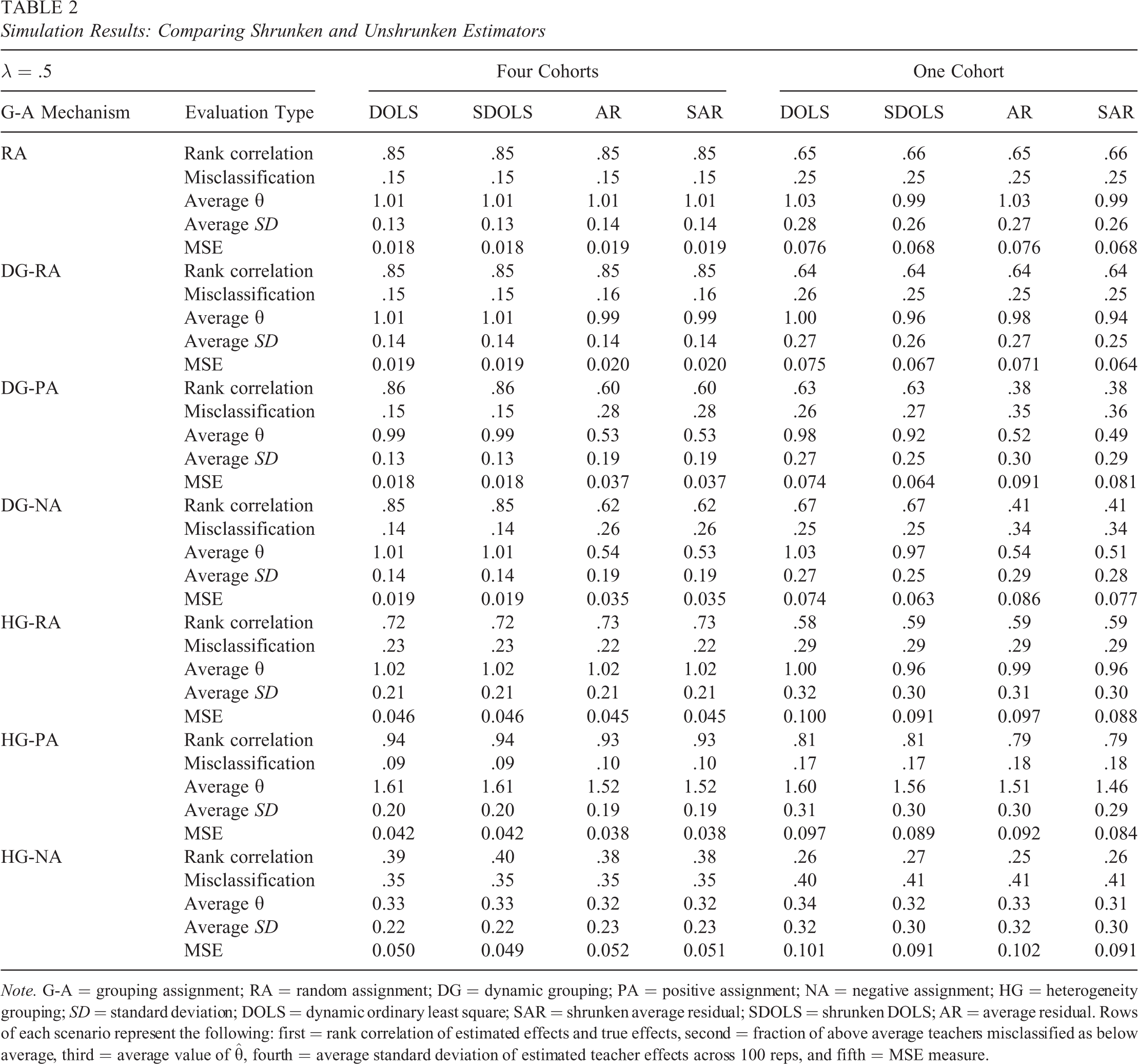
Note. G-A = grouping assignment; RA = random assignment; DG = dynamic grouping; PA = positive assignment; NA = negative assignment; HG = heterogeneity grouping; SD = standard deviation; DOLS = dynamic ordinary least square; SAR = shrunken average residual; SDOLS = shrunken DOLS; AR = average residual. Rows of each scenario represent the following: first = rank correlation of estimated effects and true effects, second = fraction of above average teachers misclassified as below average, third = average value of $\hat{θ}$ , fourth = average standard deviation of estimated teacher effects across 100 reps, and fifth = MSE measure.

5.1. Fixed Teacher Effects Versus Random Teacher Effects

In Table 1, we first compare the performance of the DOLS estimator, which treats teacher effects as fixed parameters to estimate, to the AR and EB LAG estimators that treat teacher effects as random. Under non-RA of teachers, we expect DOLS, which explicitly controls for teacher assignment through the inclusion of teacher assignment indicators, to perform better than those estimators treating the teacher effects as random. When teacher assignment is based on the lagged test score, DOLS directly controls for the assignment mechanism by including both the lagged score and teacher dummies and should perform well in this case. The simulation results presented here largely support this hypothesis.

5.1.1. Random assignment

We begin with the pure RAcase (i.e., the case of no teacher sorting), where EB-type estimation methods are theoretically justified. The results of the RA case are given in the top panel of Table 1, and they suggest very little substantial difference between the performance of the fixed and REs estimators under this scenario. As the theory suggests, EB LAG performs well in the four-cohort case, with rank correlations between the estimated and the true teacher effects near .86, which is nearly the same as the .85 rank correlation for DOLS and AR. In addition to very similar rank correlations, the misclassification rates are very similar across the three estimators, with about 15% of above-average teachers misclassified as below average. These estimators also misclassify 28% of the teachers who should be classified in the bottom quintile. The similarities between the three estimators in terms of rank correlation and misclassification rates remain when using only one cohort. Reducing the amount of data used to estimate the teacher effects lowers the performance of all estimators, decreasing the rank correlations and increasing the misclassification rates. With one cohort, rank correlations between the estimated and true teacher effects are about .65 to .67, and between 25% and 26% of above-average teachers are misclassified as below average.

In addition to rank correlations and misclassification rates, we also examine the bias and precision of the estimators. While DOLS and AR appear to be unbiased with average $\hat{θ}$ values close to 1, EB LAG substantially underestimates the magnitudes of the true teacher effects with an average $\hat{θ}$ value of .78 using four cohorts and .49 using one cohort. This bias is likely the result of the shrinkage technique that is applied, but this shrinkage does cause EB LAG to be slightly more precise than AR or DOLS. While DOLS and AR both have similar average standard deviations of the estimated teacher effects near .13 and .27 in the four- and one-cohort cases, respectively, EB LAG has lower average standard deviations of .12 and .18, respectively. Given the precision gain in EB LAG, the MSE measure suggests that EB LAG may be preferred to DOLS or AR under RA.

We now move to the cases where the students are nonrandomly grouped together, but teachers are still randomly assigned to classrooms. We allow for nonrandom grouping based on either the prior year test score (DG) or the student-level heterogeneity (HG). Under these DG-RA and HG-RA scenarios in Table 1, we see a fairly similar pattern as in the RA scenario, although the overall performance of all estimators is somewhat diminished, especially in the HG-RA scenario.

5.1.2. DG and non-RA

The performance of the various estimators diverges noticeably under nonrandom teacher assignment. We continue to nonrandomly group teachers as described previously but now allow for non-RA of students to teachers. Classes with high test scores or high unobserved ability can be assigned to either the best (PA) or the worst (NA) teachers. A key finding of this analysis is the disparity in performance between the DOLS estimator and estimators that fail to allow for correlation between the teacher assignment and the assignment mechanism (e.g., AR and EB LAG). These results suggest that, when there is nonrandom teacher assignment based on the prior test score, estimators explicitly controlling for the teacher assignment should be preferred.

Similar results hold for both DG-PA and DG-NA, so we focus only on the DG-PA results here. Under the DG-PA scenario, DOLS substantially outperforms AR and EB LAG. When using four cohorts, DOLS has a rank correlation of .86 under DG-PA, while AR and EB LAG have rank correlations of .60 and .76, respectively. AR and EB LAG also have large misclassification rates, with 28% to 32% of above-average teachers being misclassified as below average compared with only 23% for DOLS. Although not listed in the table, DOLS also misclassifies fewer teachers in the bottom quintile—DOLS only misclassifies 28% of the teachers who should be classified in the bottom quintile, while EB LAG and AR misclassify 39% and 49%, respectively.

In addition to misclassifying and poorly ranking teachers, the AR and EB LAG methods also underestimate the magnitudes of the true teacher effects. While DOLS has an average $\hat{θ}$ value of .99, the AR and EB LAG estimators have average $\hat{θ}$ values of .53 and .49, respectively. While some of the bias of the EB LAG estimates can be attributed to shrinkage, the larger issue is the bias caused by the failure of the AR and EB LAG approaches to allow for correlation between the lagged test score (i.e., the assignment mechanism in these scenarios) and the teacher assignment, a correlation that DOLS explicitly allows for with the inclusion of teacher dummies in the regression. Which estimator is preferred based on MSE differs depending on the number of cohorts. In the four-cohort case, DOLS, EB LAG, and AR have MSE values of .018, .037, and .024, respectively. When only one cohort is used, EB LAG has the smallest MSE of .051, while DOLS and AR have MSE values of .074 and .091, respectively. Despite the gain in precision, the average bias across all teachers (based on ${\hat{β}}_{g} - β_{g}$ ) and simulation reps in EB LAG is nearly 3 times that of DOLS. Given the poor teacher rankings for EB LAG in this case, the consequences of the extreme bias cannot be ignored, even if the MSE measure suggests it should be preferred.

These simulation results also verify an important result of the theoretical discussion, that is, The performance of EB LAG approaches the performance of DOLS as the number of students per teacher grows. We see less of a disparity in the performance of DOLS and EB LAG when computing VAMs using four cohorts compared to one, but the relative performance of AR does not improve with more students per teacher. For example, under DG-PA with one cohort of students, AR and EB LAG have rank correlations of .38 and .45, respectively, compared to .63 for DOLS. With four cohorts of students, the rank correlation for EB LAG is much closer to that for DOLS (.76 and .86, respectively) than is the rank correlation for AR (.60). This theoretical result is also applicable to the SAR estimator we examine below, which is used as a simpler way to operationalize the EB approach. In summary, EB LAG, which uses REs estimation in the first stage, is preferred to AR under nonrandom teacher assignment, as the EB estimates approach the preferred DOLS estimates that treat teacher effects as fixed.

5.1.3. HG and non-RA

As a final scenario, we examine the case of nonrandom teacher assignment to students grouped on the basis of student-level heterogeneity. The results for these HG scenarios are especially unstable: All estimators do an excellent job ranking teachers under positive teacher assignment and a very poor job under negative teacher assignment. In the HG-PA case with four cohorts of students, the magnitudes of the estimated VAMs are amplified as seen by the large average values for $\hat{θ}$ between 1.43 and 1.61. This improves the ability of the various estimators to rank teachers as evidenced by the high-rank correlations of about .94 for all estimators. The EB LAG estimator performs the best in this scenario, as it performs as well as the other estimators in terms of ranking and misclassification of teachers but has the smallest MSE measure. Under HG-NA with four cohorts, the performance of all estimators falls substantially, largely caused by severely underestimated teacher effects ( $\hat{θ}$ values between .15 and .33). These compressed teacher effect estimates make it difficult to rank teachers in this scenario, resulting in low-rank correlations for all estimators between .38 and .41. Just as in the HG-PA scenario, the performance of the three estimators under HG-NA is very similar across the evaluation measures we examine.

Why is the performance of DOLS, AR, and EB LAG so similar under HG-PA and HG-NA, while differing so greatly under DG-PA and DG-NA? Despite correlation between the baseline test score and the student fixed effect, the lagged test score appears to be a weak proxy for the assignment mechanism in the HG scenarios. Since none of the three estimators do well at allowing for the correlation between the assignment mechanism and the teacher assignment in these cases, the distinction between estimators that include teacher FE and those that treat teacher effects as random is less stark. As found in Guarino et al. (2015), a gain score estimator with student FE included is the most robust in these HG scenarios, as it does allow for the correlation between the assignment mechanism (i.e., student fixed effect) and the teacher assignment (i.e., teacher dummy variables). Their results lend further support to the conclusion that allowing for this correlation is extremely important in the performance of these value added estimators when there is non-RA.

5.2. Shrinkage Versus Nonshrinkage Estimation

Use of EB and other shrinkage estimators is often motivated as a way to reduce the noise in the estimation of teacher effects, particularly for teachers with a small number of students. Greater stability in the estimated effects is thought to reduce misclassification of teachers. We observed in Section 3.1 that EB LAG was generally outperformed by the FE estimator, DOLS. However, under nonrandom teacher assignment, we are unable to tell how much of the bias in the EB LAG estimator is due to treating the teacher effects as random and how much is due to the shrinkage procedure. To examine the effects of shrinkage itself, we compare the performance of unshrunken estimators, DOLS and AR, with their shrunken versions, SDOLS and SAR, in Table 2. Although SDOLS is not a commonly used or theoretically justified estimator, we explore it here to identify whether shrinking teacher fixed effect estimates could be useful in practice.

Our simulation results show that there is no substantial improvement in the performance of the DOLS or AR estimators after applying the shrinkage factor to the estimates. Using four cohorts of students, the performance measures for DOLS and AR compared to their shrunken counterparts are nearly identical to two decimal places across all grouping and assignment scenarios. Even with very limited data per teacher in the one-cohort case, when we would expect shrinkage to have a greater effect on the estimates, we find very little change in the performance of the estimators after the shrinkage factor is applied.

In the one-cohort case, shrinking either the DOLS or AR estimates slightly decreases (in the second decimal place) both the average $\hat{θ}$ values and average standard deviation of the estimated teacher effects. This increased bias in the estimates is expected when applying the shrinkage factor and, depending on the scenario and estimator we examine, the effect of this precision-bias trade-off may increase or decrease the MSE measure when comparing the shrunken and unshrunken estimates. Shrinking the DOLS and AR estimates generally reduces the MSE, due to increased precision, but makes no substantial difference on the misclassification rate of teachers, regardless of which misclassification rate we use.

The effect of shrinkage itself does not appear to be practically important for properly ranking teachers or to ameliorate the performance of the biased AR estimator found in the DG-PA and DG-NA scenarios. Given that shrinking the AR estimates does little to mitigate the performance drop of AR under DG-PA and DG-NA, our evidence suggests that shrinking the DOLS estimates is preferred to the AR estimates, if such techniques are desired.

5.3. Sensitivity Analyses

As mentioned in Section 4.1, we also test the sensitivity of these results by changing some of the parameters of the model. First, we increase the standard deviation of the distribution from which the true teacher effects are drawn. As expected from the discussion in Section 2, when teacher effects are “large” EB LAG performs similarly to DOLS, while the AR method continues to suffer in performance under the DG-PA and DG-NA scenarios. Second, we allow for more nonrandomness (i.e., decrease the amount of noise) in the assignment of teachers into classrooms. As the assignment of teachers becomes more deterministic, the performance of AR and EB LAG suffers even more in terms of lower rank correlations and higher misclassification rates than what is observed in the results in Tables 1 and 2. Given that some models use multiple prior test scores (e.g., the Education Value-Added Assessment System, or EVAAS, and the methods used by the Value-Added Research Center, or VARC), we also estimate DOLS, AR, and EB LAG with multiple lagged test scores as a sensitivity analysis. Although adding multiple lags improves the performance of AR and EB LAG in the RA case, the performance of these estimators is still outperformed by DOLS in the DG-PA and DG-NA scenarios. As a final sensitivity test, we include a peer effect (e.g., average c_i of student’s classmates) in the underlying DGP. Even when peer effects are included, EB LAG and AR continue to suffer in performance under the DG-PA and DG-NA cases.

6. Comparing VAM Methods Using Real Data

We also apply these estimation methods to actual student-level test score data and examine the rank correlations between the estimated teacher effects of the various estimators for each school district. In addition to rank correlations, we also examine whether teachers are being classified in the extremes uniformly across all of the estimators we examine. Although the real data do not allow comparison between the estimated effects and the true teacher effects, we are able to make comparisons between the estimated effects of the different estimators. This comparison provides a measure of the sensitivity of the estimated teacher effects to specifications that shrink the estimates and/or treat the teacher effects as random or fixed. The results of this analysis provide some perspective on the impact of shrinking and EB methods in a real-world setting.

6.1. Data

We apply the five methods described in Section 3 to data from an anonymous southern U.S. state. While state teacher evaluation systems often compute value added for all teachers in the state, it is not uncommon for districts to conduct their own value added analyses for high-stakes decision making. Statewide computation of value added applies a one-size-fits all approach, choosing one estimator for teachers in all districts while largely ignoring the differences in assignment mechanisms across districts. Thus, within-district value-added calculations may better rank teachers than statewide systems. To compare with our simulated analysis, we estimate teacher effects district by district using Equation 30, with math test scores as the dependent variable and controls for various student characteristics and dummies for the year. Student characteristics include race, gender, disability status, free/reduced price lunch eligibility, limited English proficiency status, and the number of student absences from school. Given that the simulations do not include student characteristics, we also conduct a sensitivity analysis that omits these variables.

The data span 2001 through 2007 and Grades 4 through 6, but the test scores from the annual assessment exam administered by the state are collected for each student from Grades 3 through 6. The data set includes 1,488,253 total students from which we have at least one current year score and one lagged score. Only 482,031 students have test scores for all grades. For simplicity and comparison with the simulation results, we estimate the value-added measures for the 20,749 unique teachers with fifth-grade students in the 67 districts, but again teachers receive multiple cohorts of students. While the average number of cohorts per teacher across the 67 districts is 3.88, we do observe 39% of teachers for only 1 year and an additional 20% of teachers for 4 or more years. On average, teachers have about 25 students per year, with only a small percentage (less than 2%) teaching more than 30 students per year. The high percentage of teachers that we observe for only 1 year could motivate researchers to employ shrinkage and EB estimators as a way to reduce precision problems due to minimal data. While there are seven very large districts with over 800 fifth-grade teachers, the average number of fifth-grade teachers in the other 60 districts is 172. In addition, 18 of the 67 districts have less than 36 total fifth-grade teachers (the number we use in the simulation), suggesting that the simulation results are comparable to many of the smaller districts in the state. It is key to note that our sensitivity analysis that increased the number of simulated teachers to 72 yielded similar results, suggesting that our simulation is also representative of larger districts.

6.2. Results

Figure 1 presents box plots that depict the distributions of the within-district rank correlations between the various lagged score estimators, DOLS, SDOLS, AR, SAR, and EB LAG. The results presented here are for math scores, but the results are similar when reading scores are used. The results presented here also include student characteristics. Although there is no change in the overall conclusions if these are omitted, the distributions between all of the estimators are slightly more dispersed. As in the discussion of the simulation results, we first compare the DOLS estimator, which treats the teacher effects as fixed, with the estimators that treat the teacher effects as random. Comparing DOLS and AR, we find that the median rank correlation is around .99, but there are nine districts with rank correlations below .90 and two districts with correlations below .50. We also observe a slightly lower median rank correlation between DOLS and EB LAG, at around .97, with five districts with rank correlations below .90 and three below .50. These results are not inconsistent with our simulation results: The performance of DOLS, AR, and EB LAG is very similar under cases of RA of teachers to classrooms, but the performance of AR and EB LAG is substantially different from DOLS under non-RA based on prior test scores. Thus, it could be the case that these outlier districts observed in the left tails of the top two box plots may be composed of schools that engage more heavily in non-RA of teachers to classrooms.

Figure 1.

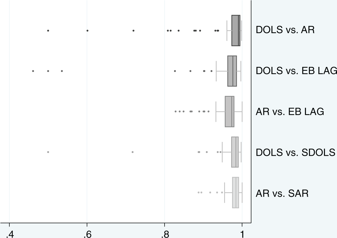
Spearman rank correlations across different value-added modeling (VAM) estimators.

Comparing the two estimators that do not explicitly control for the teacher assignment, AR and EB LAG, we find that while the median rank correlation is .96, nine districts have rank correlations of between .82 and .92. These results suggest that the estimates are somewhat sensitive to how the teacher effects are calculated in the first stage. This was also the case in the simulated results, where the performance of the AR estimator suffered more than the performance of the EB LAG estimator in cases of non-RA based on the prior test score.

For a thorough comparison with the simulation results, we also compare the shrunken and unshrunken estimates of DOLS and AR using the real data. We find median rank correlations of around .97 for both the DOLS and SDOLS comparison and the AR and SAR comparison, suggesting that shrinkage has a small impact on the estimates. It appears that in certain cases, shrinkage may have a larger impact on the DOLS estimates, as two districts have rank correlations of .50 and .72. Our simulation results suggested that shrinking the estimates had very little impact on estimator performance.

In addition to rank correlation comparisons, we also examine the extent to which teachers are classified in the tails of the distribution by the different estimators. If shrinkage is having some effect, we would expect to see some teachers classified in the extremes to be pushed toward the middle of the distribution after applying the shrinkage factor. Table 3 lists the fraction of teachers ranked in the same quintile, either the top or bottom, by different pairs of estimators. Comparing across estimators that assume fixed teacher effects to those that assume random teacher effects, we do not see much movement across quintiles. For example, comparing DOLS to EB LAG, we find that about 91% of the teachers that are classified in the top quintile using DOLS are also in this quintile using EB LAG. This suggests that teacher assignment may not be largely based on prior student achievement or that the prior test score is a poor proxy for the true assignment mechanism. If the prior test score or other covariates insufficiently proxy for the underlying assignment mechanism, then the choice to include teacher assignment variables will matter little in how teachers are ranked.

Table 3

Fraction of Teachers Ranked in Same Quintile by Estimator Pairs

	DOLS	SDOLS	AR	SAR
Top quintile
SDOLS	.91
AR	.94	.89
SAR	.89	.94	.91
EB LAG	.87	.95	.86	.93
Bottom quintile
SDOLS	.89
AR	.96	.88
SAR	.88	.95	.89
EB LAG	.87	.98	.86	.96

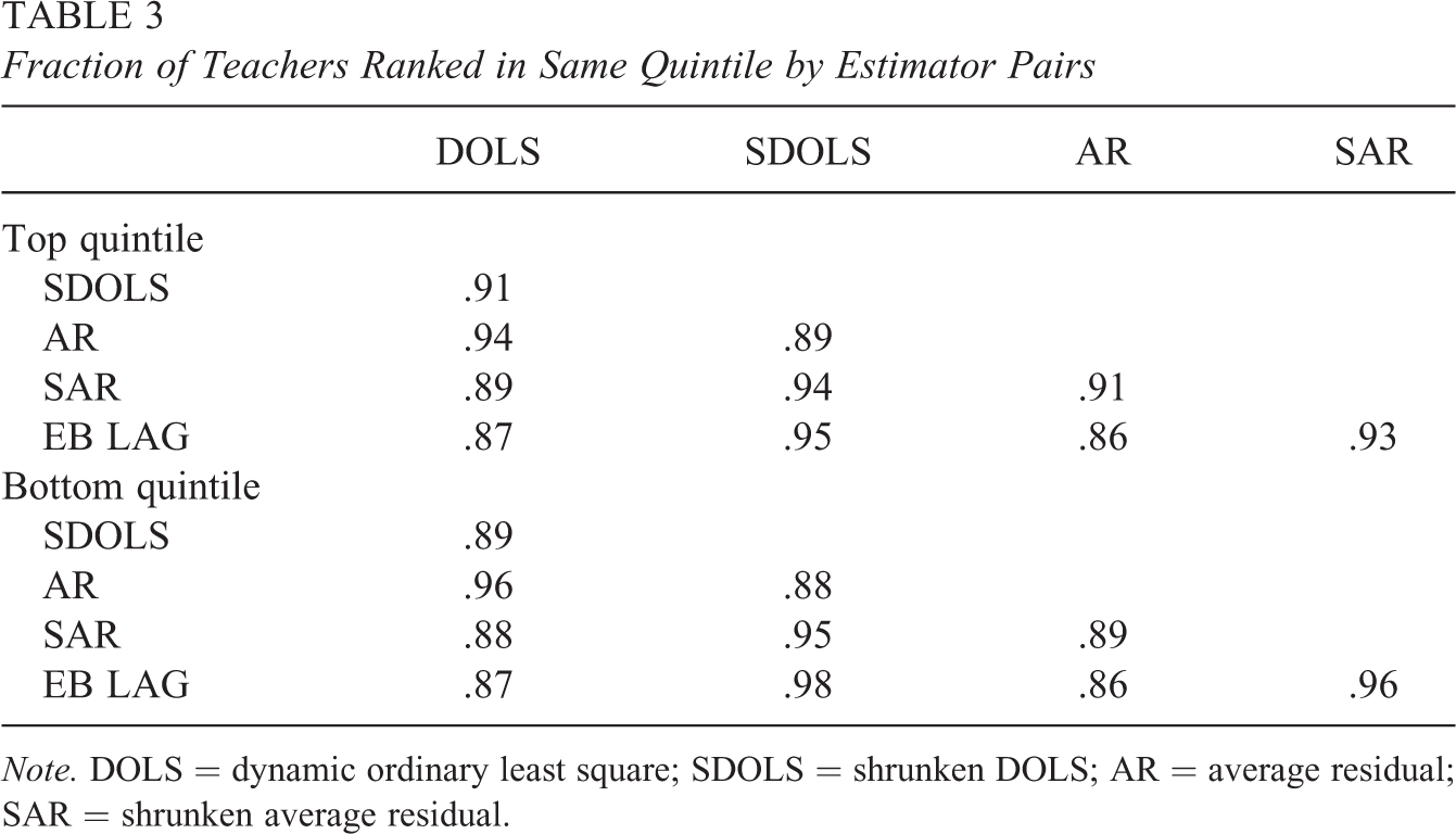
Note. DOLS = dynamic ordinary least square; SDOLS = shrunken DOLS; AR = average residual; SAR = shrunken average residual.

Comparing the rankings of unshrunken and corresponding shrunken estimators, we see that about 90% of teachers are ranked in the same quintile by both the unshrunken estimators (DOLS and AR) and their shrunken counterparts (SDOLS and SAR). This suggests that shrinking the estimates results in some reclassification of teachers in the tails to quintiles in the middle of the distribution. Using real data, however, we are unable to tell whether this reclassification is appropriate. Our simulated analysis suggested that shrinking the estimates had little impact if any on misclassification rates.

7. Conclusion

Using simulation experiments where the true teacher effects are known, we have explored the properties of two commonly used EB estimators as well as the effects of shrinking estimates of teacher effects in general. Overall, EB methods do not appear to have much advantage, if any, over simple methods such as DOLS that treat the teacher effects as fixed, even in the case of random teacher assignment where EB estimation is theoretically justified. Under RA, all estimators perform well in terms of ranking teachers, properly classifying teachers, and providing unbiased estimates. EB methods have a very slight gain in precision compared to the other methods in this case.

We generally find that EB estimation is not appropriate under nonrandom teacher assignment. The hallmark of EB estimation of teacher effects is to treat the teacher effects as random variables that are independent (or at least uncorrelated) of any other covariates. This assumption is tantamount to assuming that teacher assignment does not depend on other covariates such as past test scores (this is also true for the AR methods). When teacher assignment is not random, estimators that either explicitly control for the assignment mechanism or proxy for it in some way typically provide more reliable estimates of the teacher effects. Among the estimators and assignment scenarios we study, DOLS and SDOLS are the only estimators that control for the assignment mechanism (again, either explicitly or by proxy) through the inclusion of both the lagged test score and teacher assignment dummies. As expected, DOLS and SDOLS outperform the other estimators in the nonrandom teacher assignment scenarios. In the analysis of the real data, we found that the rank correlations between, say, DOLS and EB LAG or DOLS and SAR are quite low for some districts, suggesting that the decision between these estimators is important. Thus, if there is a possibility of non-RA, DOLS should be the preferred estimator.

As predicted by theory and seen in the simulation results, the REs estimator, EB LAG, converges to the FE estimator, DOLS, as the number of students per teacher gets large. Therefore, it could be that EB LAG is performing well in large samples simply because the estimates are approaching the DOLS estimates. However, the AR methods, AR and SAR, do not have this property. Thus, despite the recent popularity, we strongly caution using SAR as a simpler way to operationalize the EB LAG estimator. If EB-type methods are being used, possibly as a way to control for classroom-level covariates and peer effects with minimal data (a case that we do not consider in this article), it is important to estimate the coefficients in the first stage using REs estimation, as in our EB LAG estimator, rather than OLS.

Finally, we find that shrinking the estimates of the teacher effects does not seem to improve the performance of the estimators, even in the case where estimates are based on one cohort of students. The performance measures are extremely close in our simulations for those estimators that differ only due to the shrinkage factor—DOLS and SDOLS or AR and SAR. The rank correlations for these two pairs of estimators are also very close to one in almost all districts. Also, we find in the simulations that shrinking the AR estimates, which is a popular way to operationalize the EB approach, do not reduce misclassification of teachers. Thus, our evidence suggests that the rationale for using shrinkage estimators to reduce the misclassification of teachers due to noisy estimates of teacher effects should not be given much weight. Accounting for nonrandom teacher assignment when choosing among estimators is more imperative.

Given the robust nature of the DOLS estimator to a wide variety of grouping and assignment scenarios, it should be preferred to AR and EB methods when there is uncertainty about the true underlying assignment mechanism. If the assignment mechanism is known to be random, applying these AR and EB estimators can be appropriate, especially when the amount of data per teacher is minimal. However, given that the assignment mechanism is not likely known, blindly applying these AR and EB methods can be extremely problematic, especially if teachers are truly assigned nonrandomly to classrooms. Therefore, we stress caution in applying theses AR and EB methods and urge researchers and practitioners to be mindful of the underlying assignment mechanism when choosing between the various value-added methods.

Footnotes

Appendix

Table A3

Description of Evaluation Measures of Value-Added Estimator Performance

Evaluation Measure	Description
Rank correlation	Rank correlation between estimated teacher effect and true teacher effect
Misclassification	Fraction of above average teachers that are misclassified as below average
Average θ	Average value of $\hat{θ}$
Average SD	Average standard deviation of estimated teacher effects across the 100 simulation reps
MSE	Average value of $\hat{M S E} = {(β_{j} - {\hat{β}}_{j})}^{2}$

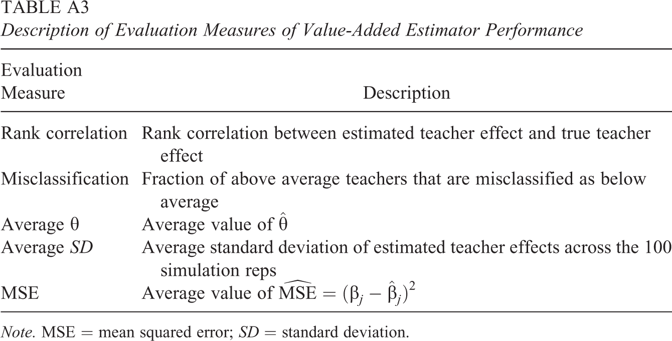
Note. MSE = mean squared error; SD = standard deviation.

Authors’ Note

The opinions expressed here are those of the authors and do not represent the views of the Institute or the U.S. Department of Education.

Declaration of Conflicting Interests

The author(s) declared no potential conflicts of interest with respect to the research, authorship, and/or publication of this article.

Funding

The author(s) disclosed receipt of the following financial support for the research, authorship, and/or publication of this article: The work here was supported by IES Statistical Research and Methodology grant #R305D10028 and in part by a Pre-Doctoral Training Grant from the IES, U.S. Department of Education (Award # R305B090011) to Michigan State University.

Notes

References

Ballou

Sanders

Wright

(2004). Controlling for student background in value-added assessment of teachers. Journal of Educational and Behavioral Statistics, 29, 37–65.

Chetty

Friedman

Rockoff

(2014). Measuring the impacts of teachers I: Evaluating bias in teacher value-added estimates. The American Economic Review, 104, 2593–2632.

Corcoran

S. P.

Jennings

J. L.

Beveridge

A. A.

(2011). Teacher effectiveness on high-and low-stakes tests. Unpublished draft.

Guarino

Reckase

M. D.

Wooldridge

J. M.

(2015). Can value-added measures of teacher education performance be trusted? Education Finance and Policy, 10, 117–156.

Hansen

C. B.

(2007). Asymptotic properties of a robust variance matrix estimator for panel data when T is large. Journal of Econometrics, 141, 597–620.

Hsiao

(2003). Analysis of panel data. Cambridge, UK: Cambridge University Press.

Jacob

B. A.

Lefgren

(2005). Principals as agents: Subjective performance measurement in education (No. w11463). Cambridge, MA: National Bureau of Economic Research.

Jacob

B. A.

Lefgren

(2008). Can principals identify effective teachers? Evidence on subjective performance evaluation in education. Journal of Labor Economics, 26, 101–136.

Kane

T. J.

Staiger

D. O.

(2008). Estimating teacher impacts on student achievement: An experimental evaluation (No. w14607). Cambridge, MA: National Bureau of Economic Research.

10.

Lockwood

J. R.

McCaffrey

D. F.

(2007). Controlling for individual heterogeneity in longitudinal models, with applications to student achievement. Electronic Journal of Statistics, 1, 223–252.

11.

McCaffrey

D. F.

Lockwood

J. R.

Koretz

Louis

T. A.

Hamilton

(2004). Models for value-added modeling of teacher effects. Journal of Educational and Behavioral Statistics, 29, 67–101.

12.

Rabe-Hesketh

Skrondal

(2012). Multilevel and longitudinal modeling using stata. 3rd ed. College Station, TX: Stata Press.

13.

Raudenbush

S. W.

(2009). Adaptive centering with random effects: An alternative to the fixed effects model for studying time-varying treatments in school settings. Education Finance and Policy, 4, 468–491.

14.

Reardon

S. F.

Raudenbush

S. W.

(2009). Assumptions of value-added models for estimating school effects. Education Finance and Policy, 4, 492–519.

15.

Rothstein

(2009). Student sorting and bias in value-added estimation: Selection on observables and unobservables. Education Finance and Policy, 4, 537–571.

16.

Rothstein

(2010). Teacher quality in educational production: Tracking, decay, and student achievement. The Quarterly Journal of Economics, 125, 175–214.

17.

Wooldridge

J. M.

(2010). Econometric analysis of cross section and panel data. 2nd ed. Cambridge, MA: MIT Press.