Assessment of Person Fit for Mixed-Format Tests

Abstract

Person-fit assessment may help the researcher to obtain additional information regarding the answering behavior of persons. Although several researchers examined person fit, there is a lack of research on person-fit assessment for mixed-format tests. In this article, the l_z statistic and the ζ₂ statistic, both of which have been used for tests with only dichotomous items or with only polytomous items, were modified for use with mixed-format tests. In a detailed simulation, the l_z and ζ₂ statistics are found to be conservative under a (frequentist) asymptotic normal approximation. However, the use of the statistics along with the (Bayesian) posterior predictive model checking method leads to a larger power. The suggested approaches are applied to an operational data set. The approaches appear to be satisfactory tools for assessing person fit for mixed-format tests.

Keywords

three-parameter logistic model generalized partial credit model item response theory model fit posterior predictive model checking

Person-fit analysis is concerned with uncovering atypical test performance as reflected in the pattern of scores on individual items in a test (Meijer & Sijtsma, 2001). Person-fit assessment may help the researcher to obtain additional information regarding the answering behavior of persons (Glas & Meijer, 2003).

Several person-fit statistics have been proposed in the context of tests with dichotomous items (see, e.g., Drasgow, Levine, & McLaughlin, 1991; Drasgow, Levine, & Williams, 1985; Klauer & Rettig, 1990; Meijer & Sijtsma, 2001; Smith, 1986; Snijders, 2001; Tatsuoka, 1984; Wright & Stone, 1979). Person-fit statistics for tests with polytomous items are less numerous (e.g., Drasgow et al., 1985; Emons, 2008; Glas & Dagohoy, 2007; van Krimpen-Stoop & Meijer, 2002; Wright & Masters, 1982).

There is a severe lack of research on person-fit assessment for mixed-format tests, which are tests that include both dichotomous and polytomous items, Finkelman and Kim (2007) being the only exception. Several examples of mixed-format tests in educational measurement (e.g., Chon, Lee, & Ansley, 2013; Kolen & Lee, 2011; Sinharay et al., 2014) show that they are quite common in the field. Further, mixed-format tests promise to become more common because of an increasing emphasis on performance tasks in the common core assessments (e.g., Darling-Hammond & Adamson, 2010, p. 1). So, it is important to be able to perform person-fit assessment for mixed-format tests. It is possible to apply the person-fit statistics designed for polytomous item response theory (IRT) models to mixed-format tests in which the Rasch model or the two-parameter logistic (2PL) model is used for the dichotomous items. This is because, as several researchers (e.g., Johnson, 2007) showed, the Rasch model and the 2PL model are special cases of the graded response model (e.g., Samejima, 1973) and also of the generalized partial credit model (GPCM; Muraki, 1992). However, these statistics cannot be applied to mixed-format tests in which the three-parameter logistic (3PL) model (or any IRT model with a guessing parameter) is used for the dichotomous items, because the 3PL model cannot be expressed as a special case of any common polytomous IRT model. The goal of this article is to fill this gap and explore several approaches for person-fit assessment for mixed-format tests.

The l_z statistic (Drasgow et al., 1985) is one of the most popular IRT-based person-fit statistics (Armstrong, Stoumbos, Kung, & Shi, 2007). Researchers such as Drasgow, Levine, and McLaughlin (1987) and Li and Olenik (1997) found the statistic to have excellent performance in comparison to other existing person-fit measures. The statistic has been applied to either tests with only dichotomous items (e.g., Drasgow et al., 1985; Glas & Meijer, 2003) or tests with only polytomous items (e.g., Drasgow et al., 1985; van Krimpen-Stoop & Meijer, 2002). The l_z statistic for mixed-format tests is defined later in this article by combining the expressions of the statistic for dichotomous items and polytomous items. The null distribution of l_z deviates substantially from the standard normal distribution for both tests with dichotomous items and tests with polytomous items—the same phenomenon is expected to occur for mixed-format tests as well.¹ It is possible to simulate data from an IRT model and compute the “empirical” null distribution of l_z from these simulated data sets, as suggested by, for example, de la Torre and Deng (2008), Meijer and Nering (1997), and Seo and Weiss (2013). However, the uncertainty in the estimated model parameters is not appropriately accounted for in this approach (e.g., Glas & Meijer, 2003, p. 218). Another possibility is to apply the posterior predictive model checking (PPMC) method (Rubin, 1984), which is a popular Bayesian approach, to find the null distribution. In fact, Magis, Raiche, and Beland (2012, p. 76) called for more research on person fit using Bayesian statistical methods. The PPMC method is applied in this article to find the null distribution of l_z .

The ζ₂ statistic was suggested by Tatsuoka (1984) for detecting aberrant response patterns that include too many correct answers to difficult items or too many incorrect answers to easy items. The ζ₂ statistic, combined with the PPMC method, was found to be the most powerful statistic among the several statistics compared in Glas and Meijer (2003). Both Tatsuoka (1984) and Glas and Meijer (2003) applied ζ₂ to tests with only dichotomous items. This article extends the statistic to mixed-format tests and employs the PPMC method to find the null distribution of ζ₂.

The next section includes a description of the l_z statistic for mixed-format tests and includes a review of the PPMC method. The section then suggests assessing person fit for mixed-format tests using the PPMC method with l_z as a test statistic. Then, the ζ₂ statistic is described in the section. In the Simulation Study section, the Type I error rate and power of l_z and ζ₂ are examined under a frequentist approach (using a standard normal null distribution) and the PPMC method in a detailed simulation study. In the Application section, the suggested approaches are applied to data from an operational test. Conclusions and recommendations are provided in the last section.

Method

The l_z Statistic for Mixed-Format Tests

Definition

The predecessor of the l_z statistic is the l statistic (Levine & Rubin, 1979) that is defined as the log likelihood of the item-level scores of a person. For a test with dichotomous items, l is defined (see, e.g., Drasgow et al., 1985; Glas & Meijer, 2003) as:

l (θ) = \sum_{k} \{Y_{k} log P_{k} (θ) + (1 - Y_{k}) log (1 - P_{k} (θ))\},

where Y_k is the examinee’s score on item k and can be either 0 or 1, and P_k (θ) is the probability of a correct answer on dichotomous item k. The statistic was expressed as a function of θ (unlike in several other articles) to stress the fact that it is a function of θ. For a test with polytomous items, l(θ) is defined (see, e.g., Drasgow et al., 1985; van Krimpen-Stoop & Meijer, 2002) as:

l (θ) = \sum_{k} \sum_{j = 0}^{m_{k}} d_{j} (Y_{k}) log P_{k j} (θ),

where Y_k , the examinee’s score on item k, is any integer between 0 and m_k , d_j (Y_k ) is an indicator function that is 1 if Y_k = j and 0 otherwise, and P_kj (θ) is the probability of a score of j on polytomous item k. Note that while both Drasgow, Levine, and Williams (1985) and van Krimpen-Stoop and Meijer (2002) assumed the same number of response categories for all polytomous items, Equation 2 allows the number to vary over the items.

Suppose that an examinee with ability θ was administered a mixed-format test consisting of K ₁ dichotomous items and K ₂ polytomous items. Combining Equations 1 and 2, the l(θ) statistic for the examinee for the test can be defined as:

l (θ) = \sum_{k = 1}^{K_{1}} \{Y_{k} log P_{k} (θ) + (1 - Y_{k}) log (1 - P_{k} (θ))\} + \sum_{k = K_{1} + 1}^{K_{1} + K_{2}} \sum_{j = 0}^{m_{k}} d_{j} (Y_{k}) log P_{k j} (θ),

where Y_k is either 0 or 1 for k = 1, 2,…, K ₁ and Y_k is any integer between 0 and m_k if k > K ₁. Note that the application of Equation 3 does not require that the first K ₁ items of the test are dichotomous—the notation, denoting the dichotomous items as items 1, 2,…, K ₁, holds for a reordering of the items in which the dichotomous items take the first K ₁ positions.²

Equation 3 implies that

\begin{aligned} E (l (θ)) = \sum_{k = 1}^{K_{1}} \{P_{k} (θ) log P_{k} (θ) + (1 - P_{k} (θ)) log (1 - P_{k} (θ))\} \\ + \sum_{k = K_{1} + 1}^{K_{1} + K_{2}} \sum_{j = 0}^{m_{k}} P_{k j} (θ) log P_{k j} (θ) \end{aligned}

and

\begin{aligned} V (l (θ)) = \sum_{k = 1}^{K_{1}} P_{k} (θ) (1 - P_{k} (θ)) {[log \frac{P_{k} (θ)}{1 - P_{k} (θ)}]}^{2} \\ + \sum_{k = K_{1} + 1}^{K_{1} + K_{2}} \sum_{j = 0}^{m_{k}} \sum_{h = 0}^{m_{k}} P_{k j} (θ) P_{k h} (θ) log P_{k j} (θ) log \frac{P_{k j} (θ)}{P_{k h} (θ)} \cdot \end{aligned}

The l_z statistic for a mixed-format test can then be defined as:

l_{z} (θ) = \frac{l (θ) - E (l (θ))}{\sqrt{V (l (θ))}} \cdot

The value of l_z (θ) decreases as the extent of person misfit increases, and a lower one-sided test is conducted to detect person misfit (e.g., Armstrong et al., 2007).

Null distribution of l_z(θ) for mixed-format tests

To apply l_z (θ) to assess the fit for a person in practice, one needs to substitute the unknown θ in Equations 3 through 5 by an estimate of θ. Let us denote an estimate of θ by $\hat{θ}$ . Let $l_{z} (\hat{θ})$ denote the value of l_z computed using $\hat{θ}$ . The uncertainty in $\hat{θ}$ leads to a problem regarding the null distribution of $l_{z} (\hat{θ})$ .

Researchers such as Molenaar and Hoijtink (1990), Nering (1995), van Krimpen-Stoop and Meijer (1999), and Snijders (2001) proved that the null distribution of $l_{z} (\hat{θ})$ for dichotomous items differs substantially from the standard normal distribution. Snijders (2001) and van Krimpen-Stoop and Meijer (1999) proved that the null distribution of $l_{z} (\hat{θ})$ is negatively skewed. As a result, the statistic often lacks power. Snijders (2001) suggested a corrected version of the $l_{z} (\hat{θ})$ statistic, referred to as the $l_{z}^{*} (\hat{θ})$ statistic, whose null distribution is closer, compared to that of $l_{z} (\hat{θ})$ , to the standard normal distribution. The $l_{z}^{*} (\hat{θ})$ statistic was found to have larger power than $l_{z} (\hat{θ})$ by researchers such as Snijders (2001) and van Krimpen-Stoop and Meijer (1999). However, $l_{z}^{*} (\hat{θ})$ was proposed only in the context of dichotomous items and its extension to polytomous items or mixed-format tests is not available yet.³

PPMC Method

Description of the method

Let the posterior distribution of the model parameters be:

p (ω | y) \propto p (y | ω) p (ω),

where y denotes the data and ω denotes the model parameters. The PPMC method (Rubin, 1984) involves assessing the fit of the model by examining whether the observed data appear extreme with respect to the posterior predictive distribution (PPD) of replicated data y ^rep, where the PPD is given by:

p (y^{r e p} | y) = \int p (y^{r e p} | ω) p (ω | y) d ω \cdot

In practice, test quantities or discrepancy measures D( y , ω) are defined (Gelman, Meng, & Stern, 1996) and the posterior distribution of D( y , ω) is compared to the PPD of D( y ^rep, ω), with substantial differences between them indicating model misfit. A researcher may use D( y , ω) = D( y ), a discrepancy measure depending on the data only (which is called a test statistic). In that case, the PPMC method consists in comparing D( y ) to the PPD of D( y ^rep). The comparison of observed and replicated discrepancy measures is mostly performed using graphical plots or using a tail-area probability referred to as the posterior predictive p value (PPP-value).

P (D (y^{r e p}, ω) \geq D (y, ω) | y) = \int_{D (y^{r e p}, ω) \geq D (y, ω)} p (y^{r e p} | ω) p (ω | y) d y^{r e p} d ω \cdot

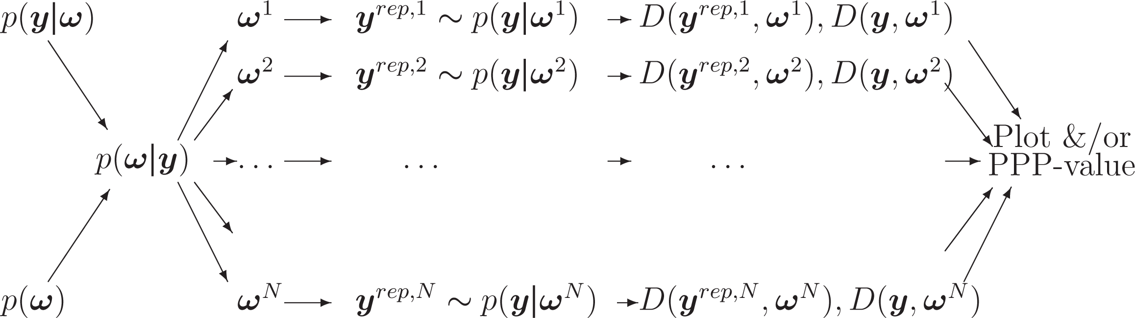
Because of the difficulty in dealing with Equations 8 and 9 analytically for all but simple problems, Rubin (1984) suggested simulating replicated (or posterior predictive) data sets from the PPD in applications of the PPMC method. One draws N simulations ω ¹, ω ², … , ω ^N from the posterior distribution $p (ω | y)$ of ω (usually with the help of a Markov chain Monte Carlo [MCMC] algorithm) and then draws y ^rep,n from the distribution $p (y | ω^{n})$ for n = 1, 2, … , N. One then computes the predictive discrepancies D( y ^rep,n, ω) and realized discrepancies D(y, ω ⁿ ), n = 1, 2, … , N. It is possible then to create a graphical plot of D( y ^rep,n, ω ⁿ ) versus D( y , ω ⁿ ), n = 1, 2, … , N, and points lying consistently above or below the 45° line indicate model misfit. The proportion of the N replications for which D( y ^rep,n, ω ⁿ ) exceeds D( y , ω ⁿ ) provides an estimate of the PPP-value. Extreme PPP-values (close to 0, 1, or both, depending on the nature of the discrepancy measure) indicate model misfit. Figure 1 graphically describes the PPMC method.

Figure 1.

A graph describing the posterior predictive model checking method.

Properties of the method and applications to educational measurement

The PPMC methods have been criticized for being conservative. The PPP-values are not necessarily uniformly distributed when the fitted model is in fact correct, and there is some evidence that PPP-values under the correct model tend to be closer to .5 more often than would be expected under a uniform distribution (Bayarri & Berger, 2000; Sinharay, Johnson, & Stern, 2006). However, researchers such as Beguin and Glas (2001), Fox and Glas (2003), Hoijtink (2001), Li, Bolt, and Fu (2006), Levy (2011), Levy, Mislevy, and Sinharay (2009), Sinharay (2005, 2006), Sinharay, Johnson, and Stern (2006), Toribio and Albert (2011), and Zhu and Stone (2011) successfully applied the PPMC method to assess various aspects of IRT model fit such as item fit, dimensionality, differential item functioning, and overall fit.

Glas and Meijer (2003) used the PPMC method to compute p-values for several person-fit statistics including the l statistic for dichotomous items but found the power of the l statistic to be low. de la Torre and Deng (2008) also applied the PPMC method with l_z for dichotomous items but found its power to be low.

Person-fit assessment using l_z and the PPMC method

In the application of the PPMC method with $l_{z} (\hat{θ})$ as a test statistic in this article, the item parameters are treated as known and equal to values from a previous calibration. Item parameters were assumed known by several researchers such as de la Torre and Deng (2008), Meijer and Nering (1997), and Snijders (2001) while performing person-fit assessment and are reasonable in several cases such as those with large sample sizes for which accurate and precise item parameter estimates are available and computerized adaptive tests in which item parameters are treated as known. In addition, Glas and Dagohoy (2007, p. 168) found that their person-fit statistics were hardly affected by whether or not the item parameters were estimated.

Let us consider the application of the PPMC method to an examinee with scores $y = (Y_{1}, Y_{2}, . . ., Y_{K_{1} + K_{2}})$ and ability parameter θ. Because the item parameters (β) are assumed to be known, the parameter vector ω in the above description of the PPMC method reduces to θ. The likelihood is given by e^l ^(θ), where l(θ) is given by Equation 3. Suppose p(θ) denote the prior distribution on θ. The prior distribution was assumed to be the standard normal distribution, as in, for example, Glas and Meijer (2003). The posterior distribution of the examinee ability, given the examinee scores, $p (θ | y)$ , is given by:

p (θ | y) \propto e^{l (θ)} p (θ) \cdot

The steps in the approach are as follows:

Compute $\hat{θ}$ , an estimate of the ability of the examinee, using y and β.

Use $\hat{θ}$ to compute the observed statistic $l_{z} (\hat{θ})$ for the examinee.

Repeat the following steps for n = 1, 2, … , N for a large N:

Generate a draw of θ from the above posterior distribution using an MCMC algorithm. Let us denote the draw by θ ⁿ .

Generate draws of scores of the examinee on all the items using β and θ ⁿ . These scores constitute y ^rep,n, the nth posterior predictive data set for the examinee.

Compute ${\hat{θ}}^{n}$ , the estimate of the ability of the examinee, using y ^rep,n and β.

Compute the statistic $l_{z}^{r e p, n} ({\hat{θ}}^{n})$ using y ^rep,n, ${\hat{θ}}^{n}$ , and β.

The above-mentioned steps lead to N replicated values of the test statistic, $l_{z}^{r e p, n} ({\hat{θ}}^{n})$ , n = 1, 2, … , N, for the examinee. Compute the PPP-value of the examinee as the proportion of times when $l_{z}^{r e p, n} ({\hat{θ}}^{n})$ is smaller than $l_{z} (\hat{θ})$ , and misfit is indicated by small PPP-values.

Note that one has to ensure that the MCMC algorithm has converged, and a sufficient number of burn-in iterations have already taken place. To perform the method for a sample of examinees, the above-mentioned steps have to be repeated separately for each examinee in the sample.

Steps 3(c) and 3(d) could be replaced by the computation of $l_{z} (θ^{n})$ and $l_{z}^{r e p, n} (θ^{n})$ using y and y ^rep,n, respectively, followed by a comparison of the two. The replacement would lead to application of the PPMC method with the discrepancy measure l_z (θ) rather than with the test statistic $l_{z} (\hat{θ})$ and represents how de la Torre and Deng (2008) and Glas and Meijer (2003) applied the PPMC method to tests with dichotomous items. However, the use of $l_{z} (θ^{n})$ and $l_{z}^{r e p, n} (θ^{n})$ is equivalent to applying the PPMC method using l as a test statistic. That is because, from Equations 4 to 6.

l_{z}^{r e p, n} (θ^{n}) < l_{z} (θ^{n}) i f a n d o n l y i f l^{r e p, n} (θ^{n}) < l (θ^{n}) .

Thus, de la Torre and Deng (2008) effectively used the l statistic with the PPMC method. It was found in initial runs that the use of (the test statistic) $l_{z}^{r e p, n} (\hat{θ})$ leads to a significantly larger power compared to the use of (the discrepancy measures) $l_{z}^{r e p, n} (θ^{n})$ or $l^{r e p, n} (θ^{n})$ .

The ζ₂ Statistic for Mixed-Format Tests

Glas and Meijer (2003) found the ζ₂ statistic (Tatsuoka, 1984) to be the most powerful discrepancy measure with the PPMC method. The ζ₂ statistic has been used only for dichotomous items and is defined as:

ζ_{2} = \frac{\sum_{k} [A_{k} (θ) - X_{k}] [A_{k} (θ) - T (θ)]}{\sqrt{\sum_{k = 1}^{K} σ_{k}^{2} (θ) [A_{k} (θ) - T (θ)]^{2}}},

where X_k is the score (0/1) on the item, A_k (θ) is defined as equal to P_k (θ), T(θ) to the average of the P_k (θ)’s, and $σ_{k}^{2} (θ)$ to $P_{k} (θ) [1 - P_{k} (θ)] .$ The index is sensitive to aberrant item score patterns with too many correct answers to difficult items and too many incorrect answers to easy items. For mixed-format tests, the statistic is defined as in Equation 11, but k goes from 1 to K ₁ + K ₂, X_k is set equal $\frac{Y_{k}}{m_{k}}$ (a fractional score), A_k (θ) to $\frac{E (Y_{k} | θ)}{m_{k}}$ , $σ_{k}^{2} (θ)$ to $\frac{V (Y_{k} | θ)}{m_{k}^{2}}$ , and T(θ) to $\frac{1}{K_{1} + K_{2}} \sum_{k = 1}^{K_{1} + K_{2}} \frac{E (Y_{k} | θ)}{m_{k}}$ . For a dichotomous item, m_k = 1 and hence $\frac{Y_{k}}{m_{k}}$ becomes the item score, $\frac{E (Y_{k} | θ)}{m_{k}}$ becomes equal to P_kj (θ) and $\frac{V (Y_{k} | θ)}{m_{k}^{2}}$ to $P_{k} (θ) [1 - P_{k} (θ)]$ . Tatsuoka (1984), who considered only dichotomous items, stated that ζ₂ may approximately follow a standard normal distribution. Therefore, the ζ₂ statistic, computed using $\hat{θ}$ and henceforth denoted as $ζ_{2} (\hat{θ})$ , was used as a test statistic with a (frequentist) standard normal approximation and also used along with the PPMC method. The above-mentioned definition of $ζ_{2} (\hat{θ})$ for mixed-format tests implies equal importance to the misfit for a dichotomous or polytomous item. Another version, providing more weight to the misfit for a polytomous item,⁴ led to poor properties and was not considered any further.

A Simulation Study

A detailed simulation study was performed to examine the Type I error rate and the power of $l_{z} (\hat{θ})$ and $ζ_{2} (\hat{θ})$ using the frequentist and the PPMC method under a variety of situations.

Design of the Simulation

The simulation study involved three levels of test length (12 items, 30 items, and 60 items) that represent short, moderate, and long tests. Each generated data set included 2-item clusters: a set of dichotomous items and a set of polytomous items. To make the compositions of mixed-format tests realistic, the proportions for each type of item were set based on the review of existing testing programs (e.g., 71% of multiple choice and 29% of constructed response items for the National Assessment of Educational Progress (NAEP) science assessment for Grades 4, 8, and 12). The number of polytomous items was 4, 10, and 20, respectively (i.e., one third), for the three test lengths. The number of response categories for each polytomous item was fixed at three with a scale ranging from 0 to 2. Because the item parameters are assumed known, the Type I error rate and the power do not depend on the number of examinees in a data set, and the number of examinees was 1,000 in each simulated data set. For each simulation condition, 1,000 data sets were generated.

Data Generation

Scores on dichotomous and polytomous items were generated using the 3PL model and GPCM, respectively. The true item parameters were generated randomly. The true slope parameters of all items were generated, as in Glas and Dagohoy (2007), from a log-normal distribution with, respectively, 0 and .25 as the mean and standard deviation of the logarithm of the variable. The true difficulty and true guessing parameters for the dichotomous items were generated from a standard normal distribution and a Uniform(0.05,0.3) distribution, respectively. The true location parameters of the polytomous items were generated from $N (- 1, 0.5)$ and $N (1, 0.5)$ distributions, respectively, as in Chon, Lee, and Dunbar (2010).

The true ability parameters were randomly drawn from the standard normal distribution. For each simulation condition, a new set of true item parameters were simulated and were then used to generate each simulated data set and in the computation of the observed and replicated values of the statistics.

To compute the Type I error of the approaches, score patterns that fit the IRT (3PL + GPCM) model were generated. To compute the power of the approaches, score patterns that are “corrupted” and do not fit the IRT model were generated in several ways. Because the item parameters are assumed known, the power does not depend on the number of examinees whose scores were corrupted—so the scores of all examinees were corrupted under each simulation condition in the “power study.”

As in other simulation studies on person-fit assessment (e.g., de la Torre & Deng, 2008; Glas & Meijer, 2003), such patterns included score patterns that are common under “lack of motivation” or “item disclosure” or “speeding.” When lack of motivation was simulated, the score patterns of all examinees involved lack of motivation to $\frac{1}{2}$ , $\frac{1}{3}$ , or $\frac{1}{6}$ of all items. It was assumed, as in Glas and Meijer (2003), that the dichotomous items on which an examinee lacks motivation are the easiest among all the dichotomous items. The probability of a correct response to a dichotomous item on which an examinee lacks motivation was set to .2 as in Glas and Meijer (2003). For a polytomous item under lack of motivation, 2.5 was subtracted from the examinee ability before generating a score—it was found on an initial run that this reduction of 2.5 was somewhat equivalent on an average to setting the probability of a correct answer to a dichotomous item to .2.⁵ When item disclosure was simulated, the score patterns of all examinees involved the assumption that $\frac{1}{2}$ , $\frac{1}{3}$ , or $\frac{1}{6}$ of all items were disclosed to the examinee. It was assumed, as in Glas and Meijer (2003), that the dichotomous items on which item disclosure occurs are the most difficult among all the dichotomous items. The probability of a correct response to a dichotomous item that was disclosed was set to 1.0 as in de la Torre and Deng (2008). The score on a “disclosed” polytomous item was set equal to the highest possible score on the item. As in de la Torre and Deng (2008), when speeding was simulated, the score patterns of all examinees involved guessing on one third of the most difficult dichotomous items and one third of the polytomous items, the probability of a correct response to a dichotomous item on which a speeding occurs was set to .20, and the ability was reduced by 2.5 before simulating a score on a polytomous item on which speeding occurs. An additional condition representing a large ability difference between the dichotomous and the polytomous items was also included. Under this condition, after generating the true ability (θ) of an examinee, the scores on the dichotomous items were simulated using θ as the ability, but the scores on the polytomous items were simulated using θ + 3 as the ability. This condition can be considered as disclosure of only the polytomous items (or much better performance on polytomous items).

Computations

Fortran 90 programs written by the author were used for the computation of maximum likelihood estimates (MLEs) of ability⁶ and implementing the Metropolis–Hastings algorithm (e.g., Gelman, Carlin, Stern, & Rubin, 2003) that was used to generate draws from the posterior distribution of ability. The proposal/jumping distribution was chosen as a normal distribution with the previous draw as the mean, and the standard deviation of the proposal/jumping distribution was chosen to ensure an acceptance of about 44% of the draws from the proposal distribution.⁷ One chain of length 4,000 was run that ensures the convergence of the algorithm and the first 1,000 draws of the chain were discarded as burn-in. The remaining draws were thinned by retaining every third draw to lead to 1,000 draws from the posterior distribution of ability for each examinee. The use of weighted likelihood estimate (WLE; Tao, Shi, & Chang, 2012, discussed the computation of WLEs for mixed-format tests), modal a posteriori (MAP), or expected a posteriori (EAP) of the ability instead of the MLE led to negligible changes in the Type I error rate and power of $l_{z} (\hat{θ})$ and $ζ_{2} (\hat{θ})$ —so only the MLE of ability is considered henceforth.

Thus, the following steps were repeated 1,000 times for any simulation condition:

Simulate a set of true item parameters.

Simulate 1,000 true ability parameters.

Use the above true item and ability parameters to simulate what would be treated as an “observed” data set.

Compute the MLE $\hat{θ}$ of all the examinees from the observed data set using the true item parameters.

Compute $l_{z} (\hat{θ})$ and $ζ_{2} (\hat{θ})$ for each examinee using $\hat{θ}$ and the true item parameters from the observed data set. Compute the frequentist p value corresponding to these statistics under a standard normal distributional assumption.

Use an MCMC algorithm to generate for each examinee 1,000 draws (after the aforementioned burn-in and thinning) from the posterior distribution of the ability.

Use the above draws of ability and the true item parameters to generate 1,000 posterior predictive data sets.

Compute the MLEs ( ${\hat{θ}}^{n}$ ) of all the examinees from the posterior predictive data sets using the true item parameters.

Compute $l_{z}^{r e p, n} ({\hat{θ}}^{n})$ and $ζ_{2}^{r e p, n} ({\hat{θ}}^{n})$ for each examinee using the estimated ability and the true item parameters from the posterior predictive data sets.

Compute the PPP-value for each examinee by comparing the $l_{z} (\hat{θ})$ and the $l_{z}^{r e p, n} ({\hat{θ}}^{n})$ ‘s and also by comparing the $ζ_{2} (\hat{θ})$ and $ζ_{2}^{r e p, n} ({\hat{θ}}^{n})$ ‘s.

Type I Error Rate

Table 1 displays the Type I error rates of the $l_{z} (\hat{θ})$ and $ζ_{2} (\hat{θ})$ statistics combined with the frequentist standard normal null distribution assumption and the PPMC method for level .05 and .01 for the three test lengths. Each value in the table is computed from one million (1,000 data sets each containing 1,000 examinees) p-values. Table 1 shows that for both $l_{z} (\hat{θ})$ and $ζ_{2} (\hat{θ})$ , the Type I error rates of the frequentist approach are substantially smaller than the nominal level, but those for the PPMC method are quite close to or equal to the nominal level.

Table 1.

Type I Error Rates From the Simulations

Test Length	Approach	Level = .05	Level = .01
12	Frequentist-l_z	.027	.007
	PPMC-l_z	.048	.009
	Frequentist-ζ₂	.036	.008
	PPMC-ζ₂	.050	.010
30	Frequentist-l_z	.031	.007
	PPMC-l_z	.049	.009
	Frequentist-ζ₂	.024	.005
	PPMC-ζ₂	.050	.010
60	Frequentist-l_z	.030	.007
	PPMC-l_z	.049	.009
	Frequentist-ζ₂	.017	.003
	PPMC-ζ₂	.050	.010

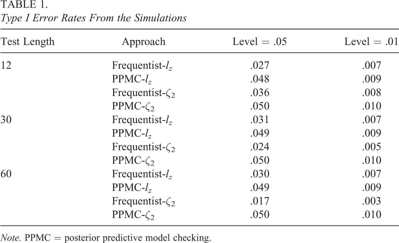
Note. PPMC = posterior predictive model checking.

The short-dashed line in Figure 2 shows the distribution of the observed values of $l_{z} (\hat{θ})$ from all the examinees from all the 1,000 simulated data sets for the simulation condition with 30 items. The solid line in the figure shows the standard normal distribution. The left tail of the distribution of $l_{z} (\hat{θ})$ is lighter than that of the standard normal distribution—so the statistic would be conservative (i.e., would have low power). Thus, the null distribution of $l_{z} (\hat{θ})$ is not standard normal for mixed-format tests. Three more lines show the distributions of the 1,000 replicated values of $l_{z} (\hat{θ})$ for three examinees for the same simulation condition. These distributions constitute the null distributions under the PPMC method. The true values of θ of these examinees are −2.3 (low), −0.1 (medium), and 2.0 (high). While all these distributions are different to a certain extent from the standard normal distribution, the distribution for the high-ability examinee is markedly different and has a smaller spread compared to the standard normal distribution—so the PPMC method will be more likely to flag such an examinee compared to a frequentist approach.

Figure 2.

Distributions of observed and replicated $l_{z} (\hat{θ})$ for the 30-item test.

Figure 3 shows the distributions of p-values from all the examinees from all the 1,000 simulated data sets for the three test lengths from the Type I error rate study. In each panel, the solid line and the dashed line, respectively, denote the distributions of the p-values for the $l_{z} (\hat{θ})$ statistic with the PPMC method and the frequentist approach. The distribution of the p-values for the $l_{z} (\hat{θ})$ combined with the PPMC method, unlike that for the frequentist approach, is quite close to the Uniform(0,1) distribution.⁸ Thus, the common criticism of the nonuniformness of the PPP-values, which leads to its conservative nature (see, e.g., Bayarri & Berger, 2000), does not apply to $l_{z} (\hat{θ})$ combined with the PPMC method. So the use of $l_{z} (\hat{θ})$ with the PPMC method would lead to a more powerful approach for person-fit assessment compared to the frequentist approach. Therefore, it is expected that the PPMC method along with $l_{z} (\hat{θ})$ will be more successful than that with l in Glas and Meijer (2003) and effectively l in de la Torre and Deng (2008).

Figure 3.

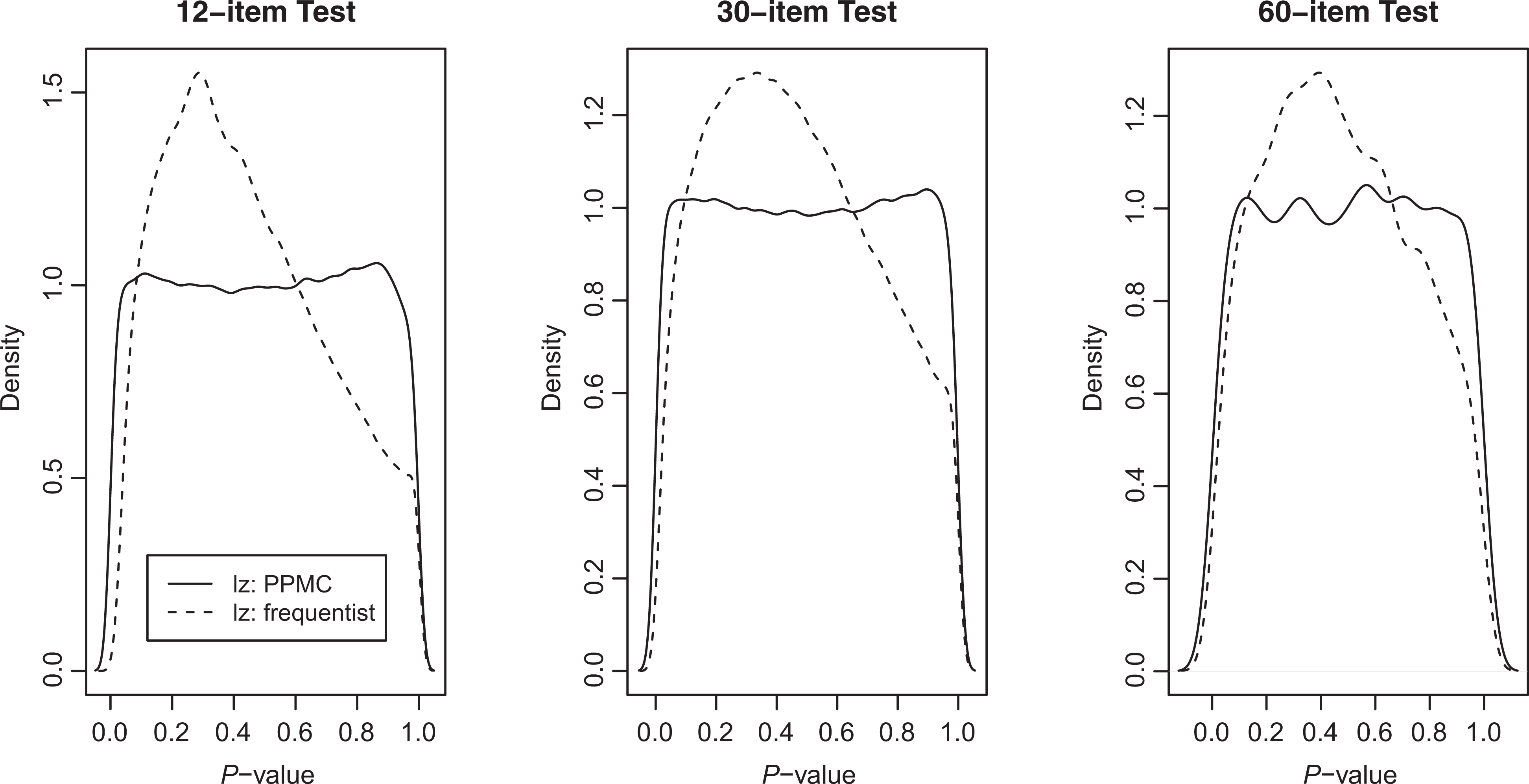
Distributions of the p-values.

Power

Table 2 presents the aggregated power values for level = .05. Columns 3 through 5 show the power of the lack of motivation conditions, Columns 6 through 8 show the power under the item disclosure conditions, Column 9 shows the power under speeding, and Column 10 shows the power when only the polytomous items are disclosed. The first four rows of numbers represent the power, for 12-item tests, for the $l_{z} (\hat{θ})$ statistic under a frequentist approach, the $l_{z} (\hat{θ})$ statistic under the PPMC method, the $ζ_{2} (\hat{θ})$ statistic under a frequentist approach, and the $ζ_{2} (\hat{θ})$ statistic under the PPMC method. Rows 5–8 represent the power for 30-item tests and Rows 9 through 12 for 60-item tests. Table 2 shows that

Table 2.

Power

Test Length	Approach	Lack of Motivation			Item Disclosure			Speeding	Disclosure of Polytomous
Test Length	Approach	$\frac{1}{6}$	$\frac{1}{3}$	$\frac{1}{2}$	$\frac{1}{6}$	$\frac{1}{3}$	$\frac{1}{2}$	Speeding	Disclosure of Polytomous
12	Frequentist-l_z	.14	.29	.29	.20	.28	.23	.03	.15
	PPMC-l_z	.20	.36	.36	.27	.37	.34	.05	.22
	Frequentist-ζ₂	.12	.30	.32	.17	.39	.42	.02	.09
	PPMC-ζ₂	.16	.36	.38	.22	.46	.48	.02	.12
30	Frequentist-l_z	.36	.50	.49	.35	.48	.42	.07	.35
	PPMC-l_z	.43	.57	.56	.42	.59	.56	.10	.50
	Frequentist-ζ₂	.28	.47	.51	.31	.63	.62	.01	.13
	PPMC-ζ₂	.42	.61	.65	.45	.74	.72	.01	.21
60	Frequentist-l_z	.58	.70	.64	.51	.61	.55	.06	.55
	PPMC-l_z	.63	.75	.73	.60	.73	.72	.08	.73
	Frequentist-ζ₂	.45	.70	.69	.53	.83	.79	.01	.16
	PPMC-ζ₂	.66	.83	.82	.75	.91	.88	.01	.27

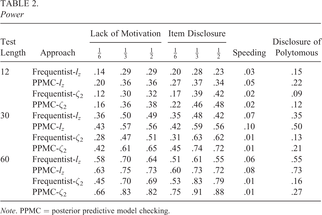
Note. PPMC = posterior predictive model checking.

The power is well below 1.0 for all test conditions. This phenomenon has been observed by several researchers such as Glas and Meijer (2003) and Meijer and Nering (1997) and is a typical feature of person-fit assessment. The power under speeding is extremely low for all the approaches, which agrees with the low power under speeding found in de la Torre and Deng (2008) for dichotomous items.

The power increases as test length increases. This is expected and is in agreement with other simulation studies such as Glas and Meijer (2003) and de la Torre and Deng (2008).

For both $l_{z} (\hat{θ})$ and $ζ_{2} (\hat{θ})$ , the power for the PPMC method is larger than or equal to that of the frequentist approach in all simulation cases, the gain ranging between .00 and .22 (for $ζ_{2} (\hat{θ})$ , 60 items, item disclosure on one sixth items). The larger power of the PPMC method agrees with the Type I error rates of the approach being close to the nominal level (Table 1). Thus, this is a rare example of the PPMC method, which is often criticized for its conservative nature (e.g., Bayarri & Berger, 2000), having larger power than the corresponding frequentist approach.

The statistic $ζ_{2} (\hat{θ})$ (either under the frequentist or PPMC method) is most often more powerful than $l_{z} (\hat{θ})$ for the lack of motivation and item disclosure conditions (especially as the proportion of corrupted responses increases) but less powerful than $l_{z} (\hat{θ})$ under the speeding and “disclosure of only polytomous items.” This is most likely because $ζ_{2} (\hat{θ})$ has high power when an examinee answers the easiest items incorrectly or most difficult items correctly, which is satisfied under the lack of motivation and item disclosure conditions. Under speeding and disclosure of only polytomous items, this condition is not satisfied because of the way data were simulated—so $ζ_{2} (\hat{θ})$ has low power.

For all test lengths, the power for $l_{z} (\hat{θ})$ increases as the proportion of items guessed or disclosed increases from 1/6 to 1/3 but decreases as the proportion increases from 1/3 to 1/2. This phenomenon was observed for some statistics and some conditions (e.g., for the T ₂ statistic for lack of motivation with sample size of 400 and test length 30) in Glas and Meijer (2003) who provided a partial explanation of the phenomenon. Let’s consider item disclosure. A person-fit statistic will have high power when the scores on a subset of items are unusual compared to the ability estimate computed from the whole test. Therefore, the power of a person-fit statistic will be increasing as the proportion-disclosed increases from 0 because the scores on the disclosed items would be unusually high compared to the examinee’s ability estimate. However, as the proportion disclosed becomes close to 1, then the ability estimate will be very high and the (high) scores on any subset of items are in consonance with the high overall ability estimate—so person-fit statistics will have low power. The same phenomenon would occur with lack of motivation as well. Therefore, as the proportion of corrupted items increases, the power of any person-fit statistic will first increase and then decrease. For $ζ_{2} (\hat{θ})$ , the power keeps increasing as the proportion of items guessed or disclosed increases from 1/6 to 1/3 to 1/2 for the 12-item tests and under lack of motivation for 30-item tests but first increases and then decreases for 60-item tests and under item disclosure for 30-item tests.

Application to Real Data

Data and Analysis

Let us consider a test that is used to measure student achievement on several subject areas in a U.S. state. Item-level scores of a random subsample of about 5,000 examinees on one form of a subject area were available. The test form includes 46 multiple-choice (and dichotomous) items and 8 constructed-response (and polytomous) items with 3 to 5 score categories. The 3PL model is used for the multiple-choice items, and the GPCM is used for the constructed-response items to obtain an estimated examinee ability. A linear transformation of the estimated ability is reported to each examinee. It is important to assess person fit for the test to obtain information on answering behavior of the examinees. The item parameters were estimated based on the subsample and used for assessing person fit. The S – χ² item-fit index (e.g., Chon, Lee, & Dunbar, 2010) were computed for all the items and the value of the statistic was significant only for 3 items. The p-values for $l_{z} (\hat{θ})$ and $ζ_{2} (\hat{θ})$ were computed using the frequentist approach (using a standard normal null distribution assumption) and the PPMC method.

Results

The proportion of extreme p-values at 5% level for $l_{z} (\hat{θ})$ is 4% for the frequentist approach and 6% for the PPMC method. The corresponding proportions for $ζ_{2} (\hat{θ})$ is 6% for the frequentist approach and 8% for the PPMC method. In order to have a deeper look, the “average fractional score” was computed for each item, where, for a multiple-choice item, the average fractional score is the proportion correct score, and, for a constructed-response item, the fractional score is the average score divided by the maximum possible score. For each examinee, the fractional score on each item was created in a similar way, where the fractional score was the original score for a multiple-choice item and the original score divided by the maximum possible score for a constructed-response item. Then, for each examinee, the two following quantities were computed:

the correlation coefficient between the examinee’s fractional scores on the items and the average fractional scores of the items. It is expected that the larger the correlation, the better is the agreement between the scores of the examinee and the scores of other examinees and the less likely it is to detect misfit for the examinee.

The items were divided in groups of five with respect to their average fractional scores. The first group included the 5 items with the smallest average fractional scores, the second group included the 5 items with the second smallest average fractional scores, and so on. For each examinee, the average fractional scores on these groups of 5 items were computed. One would expect that the average scores on these groups would increase for each examinee, that is, the average fractional score on the first group would be the smallest, and so on. Any deviation from this increasing pattern would increase the chance of the detection of misfit.

The four panels in Figure 4 show, for four examinees, the average scores for the 11 groups of items, where Groups 1 through 10 include 5 items each and Group 11 includes 4 items. The titles of the panels provide, for each examinee, the above-mentioned correlation coefficient and the p-values (denoted by the symbol “PV”) for $l_{z} (\hat{θ})$ under the frequentist approach, for $l_{z} (\hat{θ})$ under PPMC, and for $ζ_{2} (\hat{θ})$ under PPMC.

Figure 4.

Details of four examinees for the state test data.

For the first examinee, the average score on the item groups increases, and as a result, the correlation is a moderately high .36 and no misfit is detected either by the frequentist or by the PPMC method. The pattern seems to be random for the second examinee. As a result, the correlation is a modest .07 and the p value is 0 for all approaches. The pattern is increasing up to Group 7 for the third examinee, but then it fluctuates for the last four groups. As a result, the correlation is modestly negative (−.05) and the p value is 0 for all the approaches. The pattern for the fourth examinee is fluctuating for the last five groups. The correlation is .07. However, while $l_{z} (\hat{θ})$ with the frequentist approach does not indicate a significant misfit (p value is .07) at 5% level, $l_{z} (\hat{θ})$ with the PPMC method and $ζ_{2} (\hat{θ})$ under the PPMC method do (p-values are .03 and .01).

Conclusion

This article suggests four approaches for person-fit assessment for mixed-format tests. The approaches are based on the l_z statistic (Drasgow et al., 1985) and an extension of the ζ₂ statistic (Tatsuoka, 1984). A frequentist large-sample standard normal approximation of the null distribution of l_z and ζ₂ leads to a conservative assessment of person fit. However, the application of the PPMC method (Rubin, 1984) with these statistics leads to a more powerful assessment of person fit. The ζ₂ statistic was more powerful than l_z when misfit was introduced by changing the answers to the most difficult items or the easiest items, but less powerful than l_z when misfit was introduced in any other manner. In practice, it may be worthwhile to apply both l_z and ζ₂ because the nature of the aberrant response patterns for a specific data set is usually unknown.

The power of the PPMC method combined with the l_z statistic was found to be rather low in de la Torre and Deng (2008) and Glas and Meijer (2003). The better performance of l_z with the PPMC method in this article is due to the use of the estimated ability in the computation of l_z . Researchers such as Levy et al. (2009) and Sinharay (2006) found in the context of IRT models that some discrepancy measures are more powerful than others using the PPMC method. The results here show, as those in the above-mentioned articles, that although the PPMC method is conceptually straightforward, the chance of success with the method often depends on the choice of the “discrepancy measure” (or “test statistic”). Researchers such as Robins, van der Vaart, and Ventura (2000) have shown that the PPMC method is expected to lack power if the mean of the test statistic depends on the model parameters and vice versa. While the mean of l depends on θ, previous research on l_z shows that the mean of the statistic, when computed using an ability estimate such as the MLE or WLE, depends only slightly on θ.⁹ Therefore, it is no coincidence that the PPMC with l_z , where the latter is computed using the MLE of the examinee ability, was more successful than with l (de la Torre & Deng, 2008; Glas & Suarez-Falcon, 2003).

A statistically significant person-fit statistic does not necessarily mean that the corresponding examinee behaved inappropriately (e.g., cheated) during testing. It is possible, for example, that the unexpected pattern was due to fatigue, lack of motivation, or distraction during the test. Holland (1996, p. 28) stated, in the context of detection of cheating, that one can draw very limited conclusions only from a statistical test regarding the probability of cheating. That is because the test administrators can confidently claim that an examinee cheated only if “the probability that the examinee cheated given other evidence and the value of the test statistic” is very close to 1 and a significant test statistic does not necessarily imply that this probability indeed is very close to 1. Holland (1996) includes an example where, even though the test statistic is statistically significant, one could conclude that the above probability is more than .92 for one set of “the other evidence” and more than .18 for another set of the other evidence. Still, as argued in Holland (1996) in the context of the K-index for cheating detection, while the l_z or ζ₂ statistic by themselves are unable to lead to definitive statements about “the probability that the individual behaved inappropriately given other evidence and the value of the test statistic,” they can be useful as quality control procedures and can provide some evidence, when evidence from other sources are available, on possible inappropriate examinee behavior. The decision on what steps should be taken for an examinee with an aberrant response pattern will most often be made by policy makers who would most likely use other evidence on the examinees (such as the reports from the test venue) and may request recommendations or statistical evidence from psychometricians. The policy makers may choose to ignore the results regarding the test statistics, request the examinee to take the test again, or invalidate the score of the examinee.

There are several limitations of this article and, consequently, several related topics that can be further investigated. First, this article focused only on the l_z and ζ₂ statistic. The statistic $\sum_{i} (Y_{i} - E (Y_{i}))^{2} / V (Y_{i}),$ which is somewhat similar to the W-statistic used in Glas and Meijer (2003), was also considered along with the PPMC method. The Type I error rate with the statistic was satisfactory, but power was smaller overall than that of l_z . It is possible to consider several other statistics. In this article, the item parameters were treated as known and equal to values from a previous calibration. It is possible, as in Glas and Meijer (2003), to estimate item parameters and consider the effect of the estimation on the properties of the person-fit approaches suggested here. One could employ, instead of the PPMC method, the above-mentioned frequentist simulation-based approach (suggested by, e.g., de la Torre & Deng, 2008; Seo & Weiss, 2013) or the poor-person’s posterior predictive checking approach (Lee & Cai, 2011) in which draws of model parameters are simulated from an asymptotic normal approximation (with mean and variance equal to the MLE and its estimated variance, respectively) of the posterior distribution. Finally, more research on what should be done with the flagged examinees for operational tests would be quite helpful to practitioners.

Footnotes

Author’s Note

The research reported in this paper was performed when the author was an employee of McGraw-Hill Education CTB. The author is currently an employee of Pacific Metrics Corporation. Any opinions expressed in this publication are those of the author and not necessarily of McGraw-Hill Education CTB.

Declaration of Conflicting Interests

The author(s) declared no potential conflicts of interest with respect to the research, authorship, and/or publication of this article.

Funding

The author(s) received no financial support for the research, authorship, and/or publication of this article.

Notes

References

Armstrong

Stoumbos

Kung

Shi

(2007). On the performance of l_z person-fit statistic. Practical Assessment, Research, and Evaluation, 12, 1–10.

Bayarri

M. J.

Berger

J. O.

(2000). P-values for composite null models. Journal of the American Statistical Association, 95, 1127–1142.

Beguin

A. A.

Glas

C. A. W.

(2001). MCMC estimation and some fit analysis of multidimensional IRT models. Psychometrika, 66, 471–488.

Chon

K. H.

Lee

Ansley

T. N.

(2013). An empirical investigation of methods for assessing item fit for mixed format tests. Applied Measurement in Education, 26, 1–15.

Chon

K. H.

Lee

Dunbar

S. B.

(2010). A comparison of item fit statistics for mixed IRT models. Journal of Educational Measurement, 47, 318–338.

Darling-Hammond

Adamson

(2010). Beyond basic skills: The role of performance assessment in achieving 21st century standards of learning (Tech. Rep.). Stanford, CA: Stanford University, Stanford Center for Opportunity Policy in Education.

de la Torre

Deng

(2008). Improving person-fit assessment by correcting the ability estimate and its reference distribution. Journal of Educational Measurement, 45, 159–177.

Drasgow

Levine

M. V.

McLaughlin

M. E.

(1987). Detecting inappropriate test scores with optimal and practical appropriateness indices. Applied Psychological Measurement, 11, 59–79.

Drasgow

Levine

M. V.

McLaughlin

M. E.

(1991). Appropriateness measurement for some multidimensional test batteries. Applied Psychological Measurement, 15, 171–191.

10.

Drasgow

Levine

M. V.

Williams

E. A.

(1985). Appropriateness measurement with polychotomous item response models and standardized indices. British Journal of Mathematical and Statistical Psychology, 38, 67–86.

11.

Emons

W. H. M.

(2008). Nonparametric person-fit analysis of polytomous item scores. Applied Psychological Measurement, 32, 224–247.

12.

Finkelman

Kim

(2007, 4). Using person fit in a body of work standard setting. Paper presented at the Annual meeting of the American Education Research Association, Chicago, IL.

13.

Fox

J. P.

Glas

C. A. W.

(2003). Bayesian modeling of measurement error in predictor variables. Psychometrika, 68, 169–191.

14.

Gelman

Carlin

J. B.

Stern

H. S.

Rubin

D. B.

(2003). Bayesian data analysis. New York, NY: Chapman and Hall.

15.

Gelman

Meng

Stern

H. S.

(1996). Posterior predictive assessment of model fitness via realized discrepancies. Statistica Sinica, 6, 733–807.

16.

Glas

C. A. W.

Dagohoy

A. V. T.

(2007). A person fit test for IRT models for polytomous items. Psychometrika, 72, 159–180.

17.

Glas

C. A. W.

Meijer

R. R.

(2003). A Bayesian approach to person fit analysis in item response theory models. Applied Psychological Measurement, 27, 217–233.

18.

Glas

C. A. W.

Suarez-Falcon

J. C.

(2003). A comparison of item-fit statistics for the three-parameter logistic model. Applied Psychological Measurement, 27, 87–106.

19.

Hoijtink

(2001). Conditional independence and differential item functioning in the two-parameter logistic model. In Boomsma

van Duijn

M. A. J.

Snijders

T. A. B.

(Eds.), Essays in item response theory (pp. 109–130). New York, NY: Springer.

20.

Holland

P. W.

(1996). Assessing unusual agreement between the incorrect answers of two examinees using the K-index: Statistical theory and empirical support (ETS Research Report No. RR-94-4). Princeton, NJ: Educational Testing Service.

21.

Johnson

M. S.

(2007). Marginal maximum likelihood estimation of item response models in R. Journal of Statistical Software, 20, 1–24.

22.

Klauer

K. C.

Rettig

(1990). An approximately standardized person test for assessing consistency with a latent trait model. British Journal of Mathematical and Statistical Psychology, 43, 193–206.

23.

Kolen

M. J.

Lee

(2011). Psychometric properties of scores on mixed-format tests. Educational Measurement: Issues and Practice, 30, 15–24.

24.

Lee

Cai

(2011, 7). A poor person’s posterior predictive checking of structural equation models. Paper presented at the annual meeting of the Psychometric Society, Hong Kong, China.

25.

Levine

M. V.

Rubin

D. B.

(1979). Measuring the appropriateness of multiple-choice test scores. Journal of Educational Statistics, 4, 269–290.

26.

Levy

(2011). Posterior predictive model checking for conjunctive multidimensionality in item response theory. Journal of Educational and Behavioral Statistics, 36, 672–694.

27.

Levy

Mislevy

R. J.

Sinharay

(2009). Posterior predictive model checking for multidimensionality in item response theory. Applied Psychological Measurement, 33, 519–537.

28.

M. F.

Olenik

(1997). The power of Rasch person-fit statistics in detecting unusual response patterns. Applied Psychological Measurement, 21, 215–231.

29.

Bolt

D. M.

(2006). A comparison of alternative models for testlets. Applied Psychological Measurement, 30, 3–21.

30.

Magis

Raiche

Beland

(2012). A didactic presentation of Snijders’s

l_{z}^{*}

index of person fit with emphasis on response model selection and ability estimation. Journal of Educational and Behavioral Statistics, 37, 57–81.

31.

Meijer

R. R.

Nering

M. L.

(1997). Trait level estimation for nonfitting response vectors. Applied Psychological Measurement, 21, 321–336.

32.

Meijer

R. R.

Sijtsma

(2001). Methodology review: Evaluating person fit. Applied Psychological Measurement, 25, 107–135.

33.

Molenaar

I. W.

Hoijtink

(1990). The many null distributions of person fit indices. Psychometrika, 55, 75–106.

34.

Muraki

(1992). A generalized partial credit model: Application of an EM algorithm. Applied Psychological Measurement, 16, 159–176.

35.

Nering

M. L.

(1995). The distribution of person-fit using true and estimated person parameters. Applied Psychological Measurement, 19, 121–129.

36.

Robins

J. M.

van der Vaart

Ventura

(2000). The asymptotic distribution of p-values in composite null models. Journal of the American Statistical Association, 95, 1143–1172.

37.

Rubin

D. B.

(1984). Bayesianly justifiable and relevant frequency calculations for the applied statistician. Annals of Statistics, 12, 1151–1172.

38.

Samejima

(1973). Estimation of latent ability using a pattern of graded scores. Psychometrika, 38, 203–219.

39.

Seo

D. G.

Weiss

D. J.

(2013). l_z person-fit index to identify misfit students with achievement test data. Educational and Psychological Measurement, 73, 994–1016.

40.

Sinharay

(2005). Assessing fit of unidimensional item response theory models using a Bayesian approach. Journal of Educational Measurement, 42, 375–394.

41.

Sinharay

(2006). Bayesian item fit analysis for unidimensional item response theory models. British Journal of Mathematical and Statistical Psychology, 59, 429–449.

42.

Sinharay

(2015). Asymptotically correct standardization of person-fit statistics beyond dichotomous items. Psychometrika. Advance online publication. doi:10.1007/s11336-015-9465-x

43.

Sinharay

Johnson

M. S.

Stern

H. S.

(2006). Posterior predictive assessment of item response theory models. Applied Psychological Measurement, 30, 298–321.

44.

Sinharay

Wan

Whitaker

Kim

Zhang

Choi

S. W.

(2014). Determining the overall impact of interruptions during online testing. Journal of Educational Measurement, 51, 419–440.

45.

Smith

R. M.

(1986). Person fit in the Rasch model. Educational and Psychological Measurement, 46, 359–372.

46.

Snijders

(2001). Asymptotic distribution of person-fit statistics with estimated person parameter. Psychometrika, 66, 331–342.

47.

Tao

Shi

Chang

(2012). Item-weighted likelihood method for ability estimation in tests composed of both dichotomous and polytomous Items. Journal of Educational and Behavioral Statistics, 37, 298–315.

48.

Tatsuoka

K. K.

(1984). Caution indices based on item response theory. Psychometrika, 49, 95–110.

49.

Toribio

S. G.

Albert

J. H.

(2011). Discrepancy measures for item fit analysis in item response theory. Journal of Statistical Computation and Simulation, 81, 1345–1360.

50.

van Krimpen-Stoop

E. M. L. A.

Meijer

R. R.

(1999). The null distribution of person-fit statistics for conventional and adaptive tests. Applied Psychological Measurement, 23, 327–345.

51.

van Krimpen-Stoop

E. M. L. A.

Meijer

R. R.

(2002). Detection of person misfit in computerized adaptive tests with polytomous items. Applied Psychological Measurement, 26, 164–180.

52.

Wright

B. D.

Masters

G. N.

(1982). Rating scale analysis [Computer Software]. Chicago, IL: Mesa Press.

53.

Wright

B. D.

Stone

M. H.

(1979). Best test design. Chicago, IL: Mesa Press.

54.

Zhu

Stone

(2011). Assessing fit of unidimensional graded response models using Bayesian methods. Journal of Educational Measurement, 48, 81–97.

Assessment of Person Fit for Mixed-Format Tests

Abstract

Keywords

Method

The lz Statistic for Mixed-Format Tests

Definition

Null distribution of lz(θ) for mixed-format tests

PPMC Method

Description of the method

Properties of the method and applications to educational measurement

Person-fit assessment using lz and the PPMC method

The ζ2 Statistic for Mixed-Format Tests

A Simulation Study

Design of the Simulation

Data Generation

Computations

Type I Error Rate

Power

Application to Real Data

Data and Analysis

Results

Conclusion

Footnotes

Author’s Note

Declaration of Conflicting Interests

Funding

Notes

References

The l_z Statistic for Mixed-Format Tests

Null distribution of l_z(θ) for mixed-format tests

Person-fit assessment using l_z and the PPMC method

The ζ₂ Statistic for Mixed-Format Tests