A Multilevel CFA-MTMM Model for Nested Structurally Different Methods

Abstract

The numerous advantages of structural equation modeling (SEM) for the analysis of multitrait–multimethod (MTMM) data are well known. MTMM-SEMs allow researchers to explicitly model the measurement error, to examine the true convergent and discriminant validity of the given measures, and to relate external variables to the latent trait as well as the latent method factors in the model. According to Eid et al. (2008) different MTMM measurement designs require different types of MTMM-SEMs. Eid et al. (2008) proposed three different MTMM-SEMs for measurement designs with (a) structurally different methods, (b) interchangeable methods, and (c) a combination of both types of methods. In the present work, we extend this taxonomy to a multilevel correlated traits–correlated methods minus one [CTC(M − 1)] model for nested structurally different methods. The new model enables researchers to study method effects on both measurement levels (i.e., within and between clusters, classes, schools, etc.) and evaluate the convergent and discriminant validity of the measures. The statistical performance of the model is examined by a simulation study, and recommendations for the application of the model are given.

Keywords

multilevel structural equation modeling MTMM analysis structurally different and interchangeable methods

Introduction

Since Campbell and Fiske (1959) proposed a correlation-based multitrait–multimethod (MTMM) approach for the investigation of the convergent and discriminant validity of particular measures, MTMM analysis has evolved into a wide array of approaches. In the classical MTMM approach, convergent validity is represented by high correlations among different methods assessing the same trait or attribute, whereas discriminant validity is reflected by low or zero correlations between measures assessing different traits (Campbell & Fiske, 1959).

Current modeling approaches to MTMM measurement design commonly use confirmatory factor analysis (CFA-MTMM) or structural equation models (MTMM-SEMs; Brown, 2012; Eid, 2000; Eid et al., 2008; Eid, Lischetzke, Nussbeck, & Trierweiler, 2003; Eid, Lischetzk, & Nussbeck, 2006). It has been shown that MTMM-SEMs bear many advantages such as separating different components of variance from another (e.g., trait and method effects), testing theoretical assumptions via model fit indices, and/or relating latent method or trait factors to external variables (see Eid et al., 2003; Koch, Eid, & Lochner, in press; Koch, Schultze, Eid, & Geiser, 2014). Most importantly, MTMM-SEMs allow researchers to scrutinize convergent and discriminant validity on the basis of true scores (i.e., free of measurement error influences).

Over the last decades, many SEMs have been proposed for analyzing MTMM data (e.g., Dumenci, 2000; Eid, 2000; Eid et al., 2003, 2008; Kenny,1976; Kenny & Kashy, 1992; Marsh, 1993; Marsh & Hocevar, 1988; Marsh & Bailey, 1991; Pohl & Steyer, 2010; Pohl, Steyer, & Kraus, 2008; Widaman, 1985; Wothke, 1995). Today, researchers commonly use multiple instead of single indicator MTMM-SEMs, given that these models allow researchers to specify trait-specific method factors (Eid et al., 2003, 2008). Thereby, researchers may investigate whether or not method effects generalize across different traits.

Despite the growing interest in analyzing MTMM data, researchers often have difficulties selecting an appropriate MTMM model. According to Eid et al. (2008), the model selection process should be strongly guided by the particular measurement design and the type of method used in the study. Eid and colleagues argued that MTMM measurement designs can incorporate structurally different methods, interchangeable methods, or a combination of both types of methods and proposed appropriate MTMM-SEMs for each of these data structures.

Within this context, structurally different methods are methods that can be considered fixed (i.e., known or predetermined) for a particular target person. When a target is sampled from the population, these methods are given. In contrast, interchangeable methods can be randomly sampled from a target-specific pool of methods (Eid et al., 2008). For example, a person’s self-report is a fixed method once a person is sampled, but multiple colleagues’ reports can be sampled from the population of colleagues of that target. It is important to note that the term “interchangeable” does not mean that the values of the ratings are identical, but that the measurement design naturally implies a multistage sampling procedure. That is, first a target person is randomly sampled from a population of possible targets, and, secondly, multiple interchangeable methods (e.g., multiple peers’ or colleagues’ ratings) are randomly sampled from a target-specific population of interchangeable methods. In this sense, multiple peer ratings for students’ empathy can be conceived as interchangeable or random methods, whereas students’ self-reports are fixed or structurally different methods.

Eid et al. (2008) presented a single-level (classical) CFA model for measurement designs with structurally different methods, a multilevel CFA model for measurement designs with interchangeable methods, and a multilevel CFA model for measurement designs combining both structurally different and interchangeable methods. In case of structurally different methods, Eid and colleagues (2008) argued that it is reasonable using single-level (or classical) CFA models, given that structurally different methods (e.g., parents, teacher ratings, or objective tests) are fix for a particular target person (e.g., student). In contrast, Eid and colleagues proposed using multilevel MTMM-SEMs to properly model the hierarchical nature of MTMM measurement designs with interchangeable methods or with a combination of structurally different and interchangeable methods.

Since the development of this taxonomy, the models have been successfully applied to various data sets (Carretero-Dios, Eid, & Ruch, 2011; Danay & Ziegler, 2011; Geiser, Burns, & Servera, 2014) and have also been described in handbooks (Koch et al., in press). Despite the great use of this taxonomy, not all MTMM measurement designs match this framework entirely. There are many data situations in which neither one of the models is suitable.

In developmental studies, researchers often collect data from self-ratings as well as teacher ratings. In these cases, teachers rate all students within their class, making both ratings structurally different on the student level, but nested within the class. Oftentimes, the consistency between these two very different perspectives is of interest (e.g., Williford, Fite, & Cooley, 2015) or these multiple assessments are simply used as a way to ensure construct validity in measurement (e.g., Brownlie, Lazare, & Beitchman, 2012).

In organizational research, MTMM designs (termed multirater or 360° assessment) are often used to assess competencies via self- and supervisor ratings (e.g., Hannum, 2007). In these cases, the self-ratings are structurally different from supervisor ratings on the subordinates’ level, but are nested within the working group that is being supervised.

In clinical psychology and psychiatry, researchers often use self-reports and clinician-based assessment in conjunction. In this case, all clients belonging to the same clinician are rated by the same clinician. A prominent example is the assessment of depressive symptoms, where the consistency between these two assessment approaches is of focal interest (e.g., Dunlop et al., 2010; Uher et al., 2008).

Common to all of the data situations is that structurally different methods are used and that these methods are nested within higher clusters (e.g., class, team, school, etc.). Table 1 illustrates the data structure of an MTMM measurement with two nested structurally different methods (e.g., student and teacher report) and two constructs assessed by three indicators.

Table 1.

Data Format for MTMM Measurement Designs With Nested Structurally Different Methods

	Construct 1						Construct 2
	Student Reports			Teacher Reports			Student Reports			Teacher Reports
ID	Y ₁₁₁	Y ₂₁₁	Y ₃₁₁	Y ₁₁₂	Y ₂₁₂	Y ₃₁₂	Y ₁₂₁	Y ₂₂₁	Y ₃₂₁	Y ₁₂₂	Y ₂₂₂	Y ₃₂₂
1	3.75	4.06	3.88	4.67	5.20	4.14	3.16	3.65	4.45	3.88	4.53	3.79
1	3.29	3.15	2.85	4.13	4.80	4.45	3.45	3.32	3.14	4.47	4.61	4.82
1	2.72	3.27	2.68	4.71	4.16	4.05	3.22	4.13	3.42	4.78	4.58	4.94
1	3.37	2.61	2.95	3.08	3.30	2.61	3.12	2.54	2.79	2.52	2.72	2.34
1	3.04	3.29	4.15	3.63	3.85	4.20	3.11	2.63	2.69	2.54	2.32	2.32
2	4.47	4.58	4.34	3.55	2.77	3.16	2.77	2.93	2.63	3.88	2.78	2.98
2	3.15	3.35	3.25	3.15	3.60	3.14	4.01	4.43	4.46	3.75	4.01	3.44
2	2.91	4.01	3.05	2.57	2.81	3.15	2.57	3.05	2.90	3.80	3.62	3.96
2	2.56	2.86	3.69	2.33	3.25	3.83	2.97	3.48	2.79	2.46	2.73	2.65
2	3.19	2.86	3.32	3.56	3.00	3.38	2.72	2.47	2.17	3.33	2.66	3.22

Note. MTMM = multitrait–multimethod; ID = identification variable for the cluster (class, school, etc.); Y_ijk = observed variables with i = indicator, j = construct, and k method (e.g., k = 1 = students’ self-reports, k = 2 = teacher reports for a particular student); no missing values and no cross-classification assumed.

As shown in Table 1, we assume that only one teacher (or one team leader) rates all students (team members) in his or her entire class (team). Thus, for each student self-report, there is only one teacher rating, and so the class teacher and the student ratings may be conceived as structurally different methods nested within classes. Due to this fully nested data structure, teacher and student ratings may share common variance that is due to the dependencies in the data. Consequently, it would be inappropriate to use single-level MTMM-SEMs, given that the clustering in the data would be ignored under such circumstances.

Ignoring the multilevel structure can lead to serious bias of the χ² fit statistic, the parameter estimates as well as their standard errors depending on the number of observations at both levels and the level of intraclass correlation (see Julian, 2001). Numerous adjustment techniques have been proposed to correct standard errors (Huber, 1967; White, 1980) and the χ² fit statistic (Satorra & Bentler, 1994, 2001).

One shortcoming of these adjustment techniques is that the multilevel structure is not modeled explicitly, for example, by specifying latent variables at both levels (i.e., the individual level and the cluster level). Hence, even when using such adjustment techniques, the actual model would still be underspecified and no information regarding interindividual differences within and between clusters can be gathered. Especially, in educational research, it is often of great importance to model latent factors at the individual level (e.g., within classes) and at the cluster level (e.g., between classes). For example, teacher and students’ ratings may differ within and between classes and it might be of particular interest to explain teacher-related method effects at both levels (e.g., within and across classes).

In the present work, a multilevel SEM (ML-SEM) for cross-sectional MTMM measurement designs with nested structurally different models is presented. The model combines classical models of multilevel CFA (ML-CFA; Hox, 2010; B. O. Muthén, 1994) and the CTC(M − 1) approach (Eid, 2000; Eid et al., 2003, 2008). The CTC(M − 1) model can be seen as restrictive variant of the traditional correlated traits–correlated methods (CTCMs) model (Marsh & Grayson, 1995; Widaman, 1985). In the CTCM model, many trait factors and many method factors are modeled as there are traits and methods in the MTMM designs. However, in the CTC(M − 1) model, one method factor for each trait–method unit (TMU) is omitted (see Figure 1). Due to this restriction (i.e., specifying M − 1 method factors), a gold standard or reference method is chosen, to which all remaining methods are contrasted against. This kind of modeling approach has been extensively discussed in the literature of MTMM modeling (Brown, 2012; Geiser, Eid, & Nussbeck, 2008; Geiser, Eid, West, Lischetzke, & Nussbeck, 2012; Geiser et al., 2014; Höfling, Schermelleh-Engel, & Moosbrugger, 2009, Koch, Eid, & Lochner, in press; Pohl, & Steyer, 2010; Pohl, Steyer, & Kraus, 2008; Schermelleh-Engel, Keith, Moosbrugger, & Hodapp, 2004) and has also been acceptably implemented in other branches of statistical modeling, as for example, in missing data analysis (Little, Jorgensen, Lang, & Moore, 2014).

Figure 1.

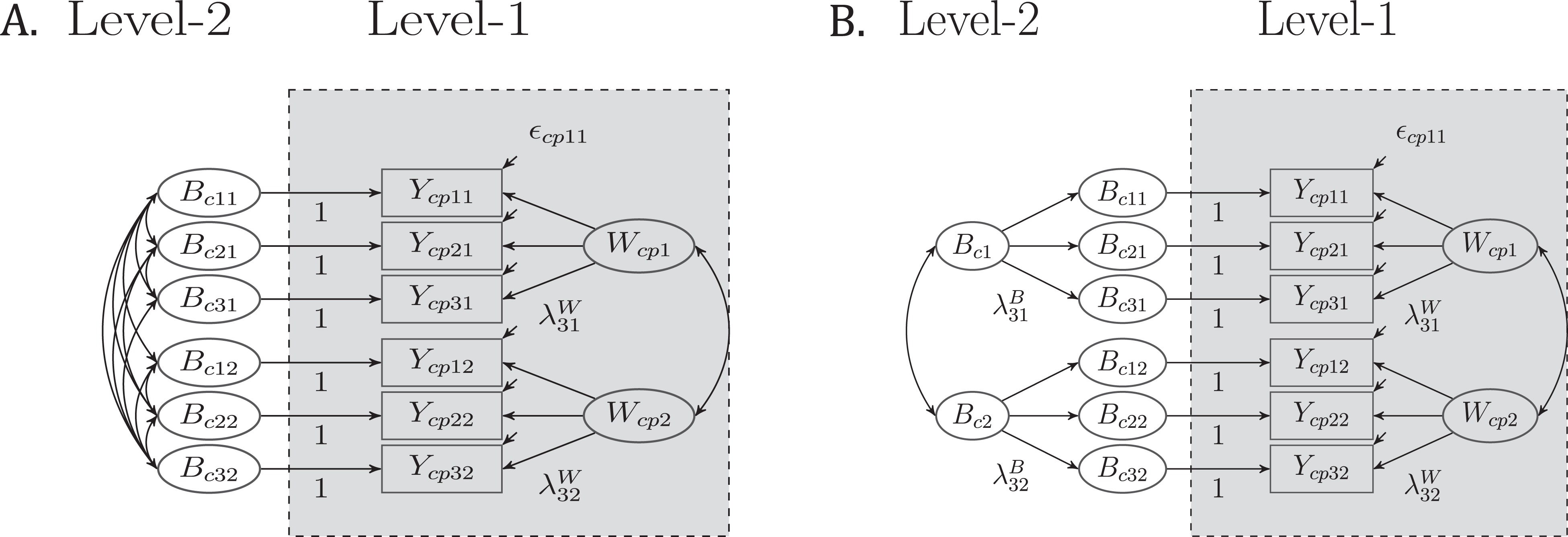
Path diagram of a multilevel confirmatory factor analysis model (see also Eid et al., 2008) with indicator-specific Level-2 factors (see Figure 1A) and with unidimensional Level-2 factors (see Figure 1B) for a multitrait–multimethod measurement design of three indicators and two constructs. Y_cpij = observed variable on Level-1 (p = person, c = cluster, i = indicator, and j = construct). B_cj = unidimensional latent factor on Level-2. W_cpj = unidimensional latent factor on Level-1. ε_cpij = Level-1 error variable. Mean structure is not presented for clarity.

One advantage of the CTC(M − 1) model is that it enables researchers to compare structurally different methods, even when different scales are used (e.g., physiological data, objective tests, questionnaires, etc.). Moreover, the CTC(M − 1) model allows researchers to separate different variance components due to trait, method, and measurement error influences and relate external variables to the latent factors in the model. Nevertheless, the multiple-indicator CTC(M − 1) model by Eid, Lischetzke, Nussbeck, and Trierweiler (2003) is limited to single-level MTMM designs with structurally different methods. The main goal of the present work is to extend the multiple-indicator CTC(M − 1) to multilevel MTMM designs with nested structurally different methods.

For simplicity, we focus on cross-sectional MTMM measurement designs with fully nested structurally different methods and do not discuss all possible extensions of the model (e.g., to cross-classified or longitudinal data structures). We report results of an empirical application as well as of a Monte Carlo (MC) simulation study investigating the trustworthiness of parameters and their standard errors for three typical design factors of two-level data structures: (a) number of Level-1 units within clusters, (b) number of Level-2 units (clusters), and (c) intraclass correlation coefficients (ICCs). The MC study was performed to identify conditions in which the model performs well with respect to these three aspects and to provide guidelines for real data applications.

Multilevel CFA-MTMM Models for Nested Structurally Different Methods

To introduce the new model, we first reconsider the basic steps of multilevel confirmatory factor models (ML-CFA) and those of MTMM-SEM of structurally different methods using the CTC(M − 1) approach (Eid, 2000; Eid et al., 2003, 2008). Then, we show how both approaches can be integrated into a general ML-CFA-MTMM model for nested structurally different methods. In addition, we clarify the meaning of the latent variables and provide formulas for estimating level-specific consistency (i.e., indicator of convergent validity) and method specificity coefficients of the measures.

ML-CFA

According to classical test theory (CTT), each observed variable Y_cpij referring to indicator i, construct j, person p, and cluster c can be decomposed as follows:

$Y_{c p i j} = τ_{c p i j} + ∊_{c p i j},$
1

where τ _cpij is the person-specific true score for indicator i, construct j in cluster c, and $∊_{c p i j}$ is the corresponding error variable. Formally speaking, τ _cpij is defined as conditional expectation of the observed variable Y_cpij given the cluster-variable p_c and the person-variable p_U , that is, $τ_{c p i j} : = E (Y_{c p i j} | p_{C}, p_{U})$ . Consequently, the error variable $∊_{c p i j}$ is defined as the difference between the observed variable Y_cpij and the person-specific true score τ _cpij , that is, $∊_{c p i j} : = Y_{c p i j} - τ_{c p i j}$ . Due to the multilevel data structure (i.e., person p is nested within cluster c), it is possible to decompose the person-specific true scores further into a latent cluster-specific variable (i.e., B_cij , between-cluster component) and a latent person-specific variable (i.e., W_cpij , within-cluster component), and representing the deviation of a particular person’s true score from the true cluster mean.

$τ_{c p i j} = B_{c i j} + W_{c p i j},$
2

where B_cij is defined as conditional expectation of the person-specific true scores τ _cpij in a cluster given the particular cluster-variable p_c (i.e., $B_{c i j} : = E (τ_{c p i j} | p_{C})$ ), and W_cpij is defined as Level-1 residual variable reflecting the deviation of a person’s true score τ _cpij from the expected true cluster mean B_cij (i.e., $W_{c p i j} : = τ_{c p i j} - B_{c i j}$ ). This approach (see Equations 1 and 2) has been referred to as implicit or latent group-mean centering in multilevel modeling (Lüdtke et al., 2008; L. K. Muthén & Muthén, 1998–2012).

Substituting Equation 2 into Equation 1 yields the measurement equation of a basic multilevel model:

$Y_{c p i j} = B_{c i j} + W_{c p i j} + ∊_{c p i j} .$
3

Note that without further restrictions the above model (see Equation 3) is not identified, because the Level-1 residual variable (W_cpij , within-cluster component) cannot be separated from measurement error $∊_{c p i j}$ influences. To identify and estimate the model in Equation 3, it is necessary to assume unidimensional within-cluster components (Eid et al., 2008):

$W_{c p i j} = λ_{i j}^{W} W_{c p j} .$
4

Equation 4 implies perfectly correlated person-specific deviations from the true cluster-specific mean. Based on this assumption, the indicator-specific within-cluster components W_cpij can be modeled by a common person-specific factor weighted by a factor loading parameter $(λ_{i j}^{W} W_{c p j})$ . Note that the factor loading parameter are assumed equal for each person p and across clusters c. Hence, the indices p and c were dropped for the factor loadings $λ_{i j}^{W}$ . The person-specific (W_cpj , within-cluster) factors are assumed to be independent and identically distributed Level-1 residual variables. As a consequence of the definition of the W_cpj factors as latent residual variables, they have an expectation (mean) of zero and are uncorrelated with any variable at Level-2 (between-clusters).

In sum, the total measurement equation for the least restrictive and identified version of an ML-CFA model is given by:

$Y_{c p i j} = B_{c i j} + λ_{i j}^{W} W_{c p j} + ∊_{c p i j} .$
5

Figure 1A represents a path diagram of the ML-CFA model shown in Equation 5, whereas Figure 1B depicts a more restrictive ML-CFA model with unidimensional cluster-specific factors using following replacement: $B_{c i j} = α_{i j}^{B} + λ_{i j}^{B} B_{c j}$ .

$Y_{c p i j} = α_{i j}^{B} + λ_{i j}^{B} B_{c j} + λ_{i j}^{W} W_{c p j} + ∊_{c p i j} .$
6

The model above (see Equation 6) resembles a classical ML-CFA model for multiple constructs (Eid et al., 2008; Hox, 2010; B. O. Muthén, 1994; Schultze, Koch, & Eid, 2015). According to Figure 1B, the model in Equation 6 assumes common factors (B_cj and W_cpj ) at both levels. In case of heterogeneous indicators (i.e., items that measure slightly different aspect of one construct), researchers should use the less restrictive model (see Equation 5) rather than the model represented in Figure 1B.

Single-level multiple indicator CTC(M − 1) models

The CTC(M − 1) modeling framework is especially useful for comparing structurally different methods (e.g., self-reports and other reports) against a reference (gold standard) method (e.g., objective or physiological measures). The basic principle of the CTC(M − 1) approach is that a gold standard or reference method is chosen and that the true scores of the nonreference methods (e.g., self-report and other reports) are predicted by the true scores pertaining to the reference method (e.g., objective or physiological measures). For choosing an appropriate reference method, researchers should generally chose the most outstanding, most valid, and most reliable method based on substantive theory or previous research findings (Geiser et al., 2008, 2012; Geiser, Koch, & Eid, 2014; Koch et al., in press). For detailed guidelines for choosing an appropriate reference method or how to specify a restricted CTC(M − 1) model that fits the data equally well regardless of the choice of the reference, see Geiser, Eid, and Nussbeck (2008).

In line with the principles of CTT, the CTC(M − 1) model can be formulated on the following basic decomposition:

$Y_{i j 1} = τ_{i j 1} + ∊_{i j 1} (reference method),$
7

$Y_{i j k} = τ_{i j k} + ∊_{i j k} (nonreference method) .$
8

The Equations 7 and 8 state that each observed variables is decomposed into a true score τ _ijk variable and a latent measurement error variable $∊_{i j k}$ . The index k was added to denote the method (e.g., k = 1 = physiological data, k = 2 = self-reports, and k = 3 other reports) used in the study.

In the next step, the true score of the nonreference methods are regressed on the true score of the reference method. That is, the CTC(M − 1) approach implies the following linear latent regression relationship:

$E (τ_{i j k} | τ_{i j 1}) = α_{i j k} + λ_{i j k} τ_{i j 1 .}$
9

The residuals of these latent linear regressions are then defined as latent method variables:

$M_{i j k} : = τ_{i j k} - E (τ_{i j k} | τ_{i j 1}) = τ_{i j k} - (α_{i j k} + λ_{i j k} τ_{i j 1}) .$
10

The latent method variables M_ijk capture the proportion of true variance of the nonreference method that cannot be predicted by the reference method. That is, the latent method variables M_ijk are defined as latent residuals with respect to the reference method of the same indicator i and construct j. As a consequence of this definition, the method variables are uncorrelated with the true score of the reference method and have an expectation (mean) of zero.

To identify and estimate the parameters in the CTC(M − 1) model, it has to be assumed that the method variables are linear transformations of each other. This assumption implies that the method variables are unidimensional across items of the same TMU and are measured by a common latent method factor. Based on this assumption, it is possible to make to following replacement:

$M_{i j k} = γ_{i j k} M_{j k} .$
11

Again, the above assumption (see Equation 11) is rather unproblematic given that in most empirical applications the method effects M_ijk will often generalize across different indicators.

In sum, the least restrictive variant of a CTC(M − 1) model with indicator-specific latent trait factors can be presented by the following measurement equations:

$Y_{i j 1} = T_{i j 1} + ∊_{i j 1} (reference method),$
12

$\begin{matrix} \begin{array}{l} Y_{i j k} = α_{i j k} + λ_{i j k} T_{i j 1} + γ_{i j k} M_{j k} + ∊_{i j k} \end{array} & (nonreference method) . \end{matrix}$
13

In the Equations 12 and 13, the true scores τ _ij ₁ of the reference method were replaced by a reference measured trait variable T_ij ₁. That means that both variables are identical and that it is not possible to separate trait- from method-specific influences with respect to the reference method within the CTC(M − 1) model framework. As Geiser et al. (2008); Geiser, Eid, West, Lischetzke, and Nussbeck (2012); as well as Geiser, Koch, and Eid (2014) clarify, a very similar approach is often used and widely accepted in ordinary regression analysis, where c − 1 dummy variables are entered into the model. Similar to ordinary regression analysis, the M − 1 method factors in the CTC(M − 1) model reflect different comparisons or contrasts, namely, the overestimation or underestimation of the true scores measured by a nonreference method that cannot be predicted by the true scores measured by the reference method. Due to this regression analytical approach, the CTC(M − 1) model allows studying method effects that are unconfounded (uncorrelated) with the reference trait (Geiser et al., 2012). Moreover, the CTC(M − 1) approach allows researchers to compare methods that were measured on different scales/metrics (Geiser et al., 2012) and to decompose the total variance of each the nonreference measured indicators into coefficients of consistency, method specificity, and reliability that will be defined below for the more general CTC(M − 1) model. Figure 2A shows a path diagram of a multiple indicator CTC(M − 1) model with three indicators, two constructs, and two structurally different methods and with indicator-specific latent trait factors. 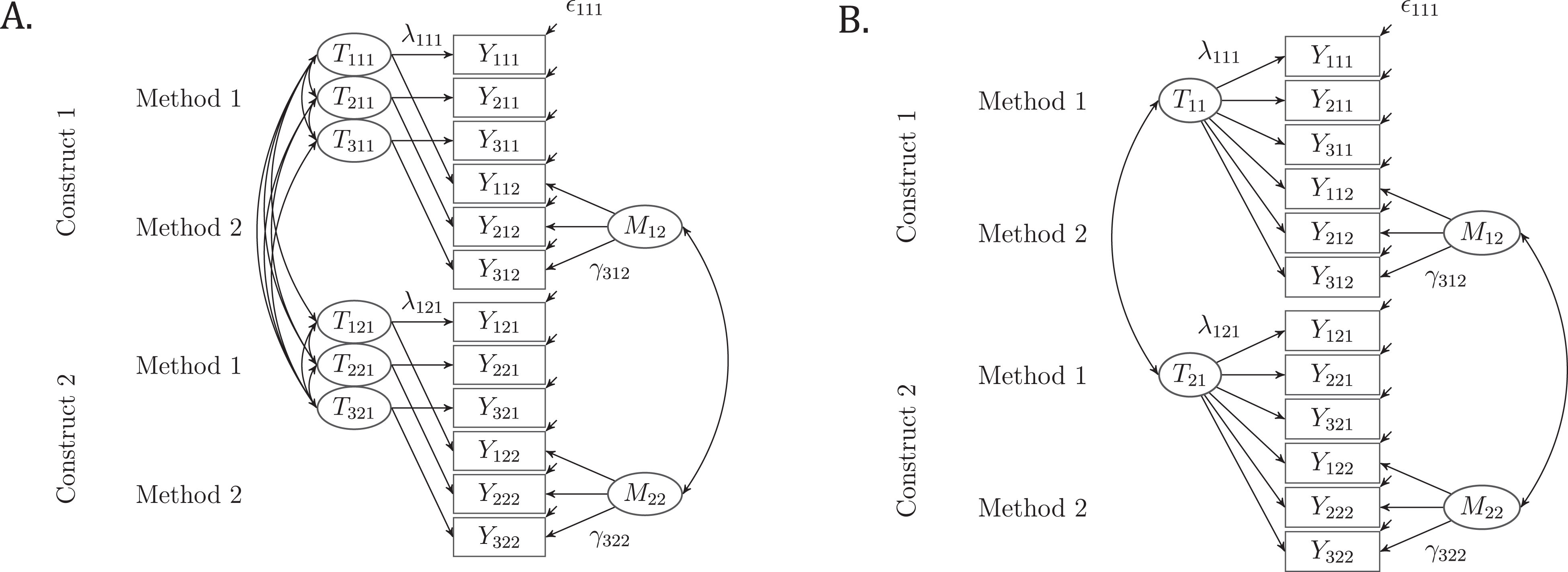Again, a more restrictive variant of the model is presented in Figure 2B, in which unidimensional latent trait factors are assumed (i.e., $T_{i j 1} = α_{i j 1} + λ_{i j 1} T_{j 1}$ ). In cases of heterogeneous indicators, we recommend to specify a CTC(M − 1) model with indicator-specific latent trait factors rather than with unidimensional latent trait factors.

Figure 2.
Path diagram of the single-level multiple indicator correlated traits–correlated methods minus one (CTC(M − 1)) model by Eid et al. (2003) with indicator-specific latent trait factors (see Figure 2A) and with unidimensional latent trait factor (see Figure 2B) for a multitrait–multimethod measurement design with three indicators, two constructs, and two (structurally different) methods. Note that in the CTC(M − 1) model one method factor is fixed to zero and only k − 1 method factors are specified. Y_ijk = observed variable (i = indicator, j = construct, and k = method). T_j ₁ = common latent trait factor. M_jk = latent method factor. ε_ijk = error variable. Mean structure is not presented for clarity.

Combining both approaches

Here we introduce the multilevel CTC(M − 1) modeling framework for fully nested structurally different methods. To apply this model, it is assumed that first a cluster (c; school, class, and team) is chosen, and, secondly, structurally different methods (k = {1, …, K}; teacher and student reports) are selected from out of each cluster, implying an MTMM measurement design with fully nested structurally different methods (see Table 1 for the implied MTMM measurement design).

Again, the starting point for defining the new model is the decomposition of the observed variables into a latent between B_cijk component and a latent within W_cpijk component. For simplicity, we assume that the within-cluster effect can be separated from measurement error influences for now¹:

$Y_{c p i j 1} = B_{c i j 1} + W_{c p i j 1} + ∊_{c p i j 1} (reference method),$
14

$Y_{c p i j k} = B_{c i j k} + W_{c p i j k} + ∊_{c p i j k} (nonreference method) .$
15

Index k was added to denote the method. The reference method (e.g., students’ self-reports) is represented by k = 1, whereas the nonreference method (e.g., teacher reports) is expressed by k ≠ 1. Subsequently, B_cij ₁ is defined as conditional expectations of the true scores τ _cpij ₁ of item i (e.g., “I enjoy studying.”) measuring construct j (e.g., intrinsic motivation) with method k = 1 (e.g., self-reports) given the cluster c (e.g., a particular class). That is, a value of B_cij ₁ can be conceived as expected true intrinsic motivation of class c measured by the first item on a students’ self-report questionnaire. W_cpij ₁ captures the true student-specific deviations from the expected true intrinsic motivation of the class (i.e., self-rated group-mean-centered intrinsic motivation of a student). For example, a positive value of W_cpij ₁ would mean that a particular student overrates his or her intrinsic motivation with regard to the expected true intrinsic motivation of the class. In contrast, B_cijk can be interpreted as the expected true intrinsic motivation of class c rated by the class teacher on the first item (e.g., “The student p enjoys studying.”). Values of W_cpijk capture the true teacher-specific deviations from the expected true intrinsic motivation of the class (i.e., teacher rated group-mean-centered intrinsic motivation of a student). Put differently, the values of W_cpijk (see Equation 15) reflect whether or not the true intrinsic motivation of a particular student is regarded as above or as below the class average by the class teacher.

In accordance with the CTC(M − 1) framework, as a reference (gold standard) method is chosen next. For simplicity, we have selected the self-reports to serve as reference method in the present study. However, it may be also reasonable to select the teacher reports as reference method. Again, detailed guidelines on choosing an appropriate reference method are provided by Geiser (2012). After choosing a reference method, latent linear regression analyses are carried out on Level-1 and -2:

$E (W_{c p i j k} | W_{c p i j 1}) = λ_{i j k}^{W} W_{c p i j 1} (Level - 1),$
16

$E (B_{c i j k} | B_{c i j 1}) = α_{i j k}^{B} + λ_{i j k}^{B} B_{c i j 1} (Level - 2) .$
17

Note that there is no intercept parameter on Level-1 (within level, see Equation 16), because the within components are defined as latent zero-mean residuals. Equation 16 states that the group-mean-centered student’s intrinsic motivation rated by the class teacher can be predicted by the self-rated group-mean-centered intrinsic motivation of that student. A positive factor loading parameter $λ_{i j k}^{W}$ indicates that an overestimation of students’ self-rated intrinsic motivation is associated with an overestimation of students’ intrinsic motivation rated by the class teacher within classes. Equation 17 states that the teacher rated true average intrinsic motivation of the class can be predicted by self-rated true average intrinsic motivation of the class.

The residuals of these latent linear regression analyses are again defined as latent method variables at both levels (Level-1 and -2):

$M_{c p i j k}^{W} : = W_{c p i j k} - E (W_{c p i j k} | W_{c p i j 1}) (Level -1),$
18

$M_{c i j k}^{B} : = B_{c i j k} - E (B_{c i j k} | B_{c i j 1}) (Level- 2) .$
19

The method variables are defined as latent residuals with respect to the reference measured within and between components (i.e., W_cpij ₁, B_cij ₁), respectively. Therefore, they are uncorrelated with their regressors and have expectations (means) of zero. The within method variables $M_{c p i j k}^{W}$ capture the proportion of variance of the teacher rated (group-mean centered) students’ intrinsic motivation corrected for the students’ self-rated (group-mean centered) intrinsic motivation within classes. Thus, the within method variables $M_{c p i j k}^{W}$ can be conceived as latent semipartial residual variables representing the true teacher view on a particular student free of measurement error influences, free of the student’s perspective, and free of class differences (due to group-mean centering). In empirical applications, this latent variable might be also linked to other variables (e.g., gender, outcome variables, and personality variables).

Following a similar logic, the between-method variables $M_{c i j k}^{B}$ reflect the proportion of true cluster-specific (i.e., between classes) variance of the teacher ratings that cannot be predicted by the students’ self-reports across classes. Again, the between-method variables $M_{c i j k}^{B}$ can be seen as latent semipartial residual variables representing the general perspective of the class teacher on his or her class free of measurement error influences and free of the students’ perspective (i.e., reference method). Positive values of the between-method variables $M_{c i j k}^{B}$ indicate that students’ true average intrinsic motivation are overestimated by their class teachers as expected by all teachers rating their classes.

To identify and estimate the CTC(M − 1) model for nested structurally different methods, unidimensional within method factors have to be assumed:

$M_{c p i j k}^{W} = γ_{i j k}^{W} M_{c p j k}^{W} (Level- 1) .$
20

Again, the above Assumption (Equation 20) is rather unproblematic and implies that within method effects (i.e., true teacher effects within classes corrected for the students’ self-reports) generalize across different indicators. Note that it is not necessary to assume unidimensional between-method factors to identify or estimate the CTC(M − 1) for nested structurally different methods. However, we generally recommend to test the following restriction by using classical model fit and model comparison statistics:

$M_{c i j k}^{B} = γ_{i j k}^{B} M_{c j k}^{B} (Level- 2) .$
21

According to Equation 21, it is assumed that the between-method effects are homogeneous across different indicators and thus can be replaced by unidimensional between-method factors $(M_{c j k}^{B})$ . Depending on whether or not the between-method factors $M_{c i j k}^{B}$ correlate strongly across different indicators i and i′ pertaining to the same method k and same construct j, this replacement can be made.

Based on the above assumptions (see Equations 20 and 21), the CTC(M − 1) model for nested structurally different methods with indicator-specific trait factors at Level-1 and -2 can then be expressed as follows:

$Y_{c p i j 1} = T_{c i j 1}^{B} + T_{c p i j 1}^{W} + ∊_{c p i j 1},$
22

$\begin{array}{l} Y_{c p i j k} = α_{i j k}^{B} + λ_{i j k}^{B} T_{c i j 1}^{B} + γ_{i j k}^{B} M_{c j k}^{B} + λ_{i j k}^{W} T_{c p i j 1}^{W} + γ_{i j k}^{W} M_{c p j k}^{W} + ∊_{c p i j k} . \end{array}$
23

For simplicity, we replaced B_cij ₁ by $T_{c i j 1}^{B}$ to denote the between-cluster trait variable and W_cpij ₁ by $T_{c p i j 1}^{W}$ to represent the within-cluster trait variable in Equations 22 and 23. Following the above example, the $T_{c i j 1}^{B}$ can be conceived as true expected intrinsic motivation of a class with respect students’ self-reports. $T_{c p i j 1}^{W}$ is the self-rated group-mean-centered intrinsic motivation of a student in a class. The part $α_{i j k}^{B} + λ_{i j k}^{B} T_{c i j 1}^{B}$ represents the latent linear regression of the teacher reports by the students’ reports at Level-2 (i.e., across classes). The part $γ_{i j k}^{B} M_{c j k}^{B}$ captures the part of the teacher reports that are not shared with the students’ reports at Level-2. Thus, the between variance of the true teacher reports (i.e., across classes) is given by:

$Var (B_{c i j k}) = (λ_{i j k}^{B})^{2} Var (T_{c i j 1}^{B}) + {(γ_{i j k}^{B})}^{2} Var (M_{c j k}^{B}) (Level- 2) .$
24

The above variance decomposition (see Equation 24) follows directly based on the definition of the latent variables and allows calculating coefficients of consistency and method specificity at Level-2:

$L2Con (B_{c i j k}) = \frac{{(λ_{i j k}^{B})}^{2} Var (T_{c i j 1}^{B})}{Var (B_{c i j k})} (Level- 2) .$
25

The Level-2 consistency coefficient reflects the proportion of the true teacher perspective that is shared by the true students’ perspective across different classes. The square root of the Level-2 consistency coefficient can be interpreted as convergent validity between the teacher and the student reports across different classes.

In contrast, the Level-2 method specificity represents the proportion of the true teacher perspective that is not shared with true students’ perspective across different classes.

$L2Msp (B_{c i j k}) = \frac{{(γ_{i j k}^{B})}^{2} Var (M_{c j k}^{B})}{Var (B_{c i j k})} (Level- 2) .$
26

Following a similar logic, coefficients of consistency and method specificity can be defined at Level-1 (i.e., within classes). Again, the variance of the true (group-mean centered) teacher reports at Level-1 can be decomposed as follows:

$Var (W_{c p i j k}) = (λ_{i j k}^{W})^{2} Var (T_{c p i j 1}^{W}) + {(γ_{i j k}^{W})}^{2} Var (M_{c p j k}^{W}), (Level- 1) .$
27

Again, the above decomposition (see Equation 27) follows directly based on the definition of latent variables. The Level-1 consistency coefficient is given by:

$L1Con (W_{c p i j k}) = \frac{{(λ_{i j k}^{W})}^{2} Var(T_{c p i j 1}^{W})}{Var (W_{c p i j k})} (Level- 1) .$
28

The Level-1 consistency coefficient reflects the proportion of the true variance of the teacher reports that can be explained (predicted) by the students’ reports within classes. Again, the square root of the Level-1 consistency coefficient is an indicator of the convergent validity of teacher and student report within classes. The Level-1 method specificity coefficient represents the proportion of the true variance of the teacher reports that cannot be explained (predicted) by the students’ reports within classes.

$L1Msp (W_{c p i j k}) = \frac{{(γ_{i j k}^{W})}^{2} Var (M_{c p j k}^{W})}{Var (W_{c p i j k})} (Level- 1) .$
29

In sum, the total variance of the observed variables can be decomposed as follows:

$Var (Y_{c p i j 1}) = Var (T_{c i j 1}^{B}) + Var (T_{c p i j 1}^{W}) + Var (∊_{c p i j 1}),$
30

$\begin{array}{l} Var (Y_{c p i j k}) = (λ_{i j k}^{B})^{2} Var(T_{c i j 1}^{B}) + (γ_{i j k}^{B})^{2} Var (M_{c j k}^{B}) + (λ_{i j k}^{W})^{2} Var (T_{c p i j 1}^{W}) \\ + (γ_{i j k}^{W})^{2} Var (M_{c p j k}^{W}) + Var (∊_{c p i j k}) . \end{array}$
31

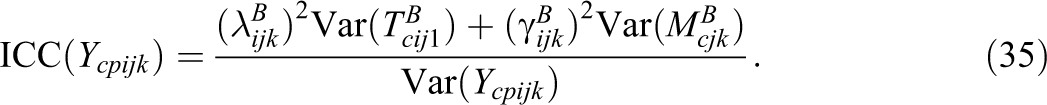
Subsequently, coefficients of the reliability (Rel) as well as the intraclass correlations (ICCs) of the observed variables can be expressed by:

$Rel (Y_{c p i j 1}) = 1 - \frac{Var (∊_{c p i j 1})}{Var (Y_{c p i j 1})},$
32

$Rel (Y_{c p i j k}) = 1 - \frac{Var (∊_{c p i j k})}{Var (Y_{c p i j k})},$
33

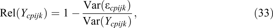
The reliability is defined as the proportion of variance of the observed variables that is not due to measurement error influences. The intraclass correlation is defined as the proportion of variance of the observed variables that is due to interindividual differences at the cluster level (Level-2). Note that the intraclass correlation coefficients can also be defined based on the variance of the true score variables (see Table 2).

Table 2.
Variance Components of the Nonreference Methods in the CTC(M − 1) Model for Nested Structurally Different Methods

Formulas Level Meaning

Level-2 consistency

$L 2 Con (B_{c i j k}) = \frac{{(λ_{i j k}^{B})}^{2} Var (T_{c i j 1}^{B})}{Var (B_{c i j k})}$ Level-2 Proportion of true variance of a nonreference method indicator that is due to reference measured trait across clusters

Level-1 consistency

$L 1 Con (W_{c p i j k}) = \frac{{(λ_{i j k}^{W})}^{2} Var (T_{c p i j k}^{W})}{Var (W_{c p o j k})}$ Level-1 Proportion of true variance of a nonreference method indicator that is due to reference measured trait within clusters

Total consistency

$TC (Y_{c p i j k}) = L 2 Con (B_{c i j k}) + L 1 Con (W_{c p i j k})$

Level-2 method specificity

$L 2 Msp (B_{c i j k}) = \frac{(λ_{i j k}^{B}) Var (M_{c j k}^{B})}{Var (B_{c i j k})}$ Level-2 Proportion of true variance of a nonreference method indicator that is not due to reference measured trait, but due to method-specific influences across clusters

Level-1 method specificity

$L 1 Msp (W_{c p i j k}) = \frac{{(λ_{i j k}^{W})}^{2} Var (M_{c p j k}^{W})}{Var (W_{c p o j k})}$ Level-1 Proportion of true variance of a nonreference method indicator that is not due to reference measured trait, but due to method-specific influences within clusters

Total method specificity

$TMS (Y_{c p i j k}) = L 2 Msp (B_{c i j k}) + L 1 Msp (W_{c p i j k})$

Intraclass correlation coefficient

$ICC (Y_{c p i j k}) = \frac{Var (B_{c i j k})}{Var (B_{c i j k}) + Var (W_{c p i j k}) + Var (∊_{c p i j k})}$ for the observed variables

$ICC (τ_{c p i j k}) = \frac{Var (B_{c i j k})}{Var (B_{c i j k}) + Var (W_{c p i j k}) + Var (∊_{c p i j k})}$ for the true score variables

Reliability

$Rel (Y_{c p i j k}) = 1 - \frac{Var (∊_{c p i j k})}{Var (Y_{c p i j k})}$ Level-1 Ratio of true variance to observed variance

Note. c = Level-2 unit (cluster), p = Level-1 unit (person), i = indicator; j = construct; k = method (reference or nonreference method); CTC(M − 1) = correlated traits–correlated methods minus one.

$ICC (Y_{c p i j 1}) = \frac{Var (T_{c i j 1}^{B})}{Var (Y_{c p i j 1})},$
34

$ICC (Y_{c p i j k}) = \frac{{(λ_{i j k}^{B})}^{2} Var (T_{c i j 1}^{B}) + {(γ_{i j k}^{B})}^{2} Var (M_{c j k}^{B})}{Var (Y_{c p i j k})} .$
35

Tables 2 and 3 summarize the formal definitions of the latent variables and the different variance coefficients in the CTC(M − 1) for nested structurally different methods.

Table 3.
Variable Definitions of the CTC(M − 1) Model for Nested Structurally Different Methods

Formulas Description Meaning

True scores and trait variables

$τ_{c p i j k} : = E (Y_{c p i j k} | p C, p U)$ True score variables on Level-1 Conditional expectation of the observed variables given the cluster and the Level-1 observational unit pertaining to a particular method (self-report, teacher reports)

$T_{c i j k}^{B} : = E (τ_{c p i j k}^{W} | p_{C})$ Trait variables at Level-2 Conditional expectation of the Level-1 true scores given the cluster (true cluster mean)

$T_{c p i j k}^{W} : = τ_{c p i j k}^{W} - T_{c i j k}^{B}$ Trait variables at Level-1 Deviation of the true scores of a structurally different method from the true cluster mean of this method (Level-1 residuals)

Linear latent regression analyses

$E (T_{c i j k}^{B} | T_{c i j 1}^{B}) = α_{i j k}^{B} + λ_{i j k}^{B} T_{c i j 1}^{B}$ Linear latent regression at Level-2 Conditional expectation of the Level-2 true scores of the nonreference method given the Level-2 true scores of the reference method

$E (T_{c p i j k}^{W} | T_{c p i j 1}^{W}) = λ_{i j k}^{W} T_{c p i j 1}^{W}$ Linear latent regression at Level-1 Conditional expectation of the Level-1 true scores of the nonreference method given the Level-1 true scores of the reference method

Method variables

$M_{c i j k}^{B} : = T_{c i j k}^{B} - E (T_{c i j k}^{B} | T_{c i j 1}^{B})$ Method variables at Level-2 Level-2 method-specific variation of a nonreference method that cannot be explained by the reference method

$M_{c p i j k}^{W} : = T_{c p i j k}^{W} - E (T_{c p i j k}^{W} | T_{c p i j 1}^{W})$ Method variables at Level-1 Level-1 method-specific variation of a nonreference method that cannot be explained by the reference method

Measurement error variables

$∊_{c p i j k} : = Y_{c p i j k} - τ_{c p i j k}$ Measurement errors at Level-1 Unsystematic variation due to measurement error influences

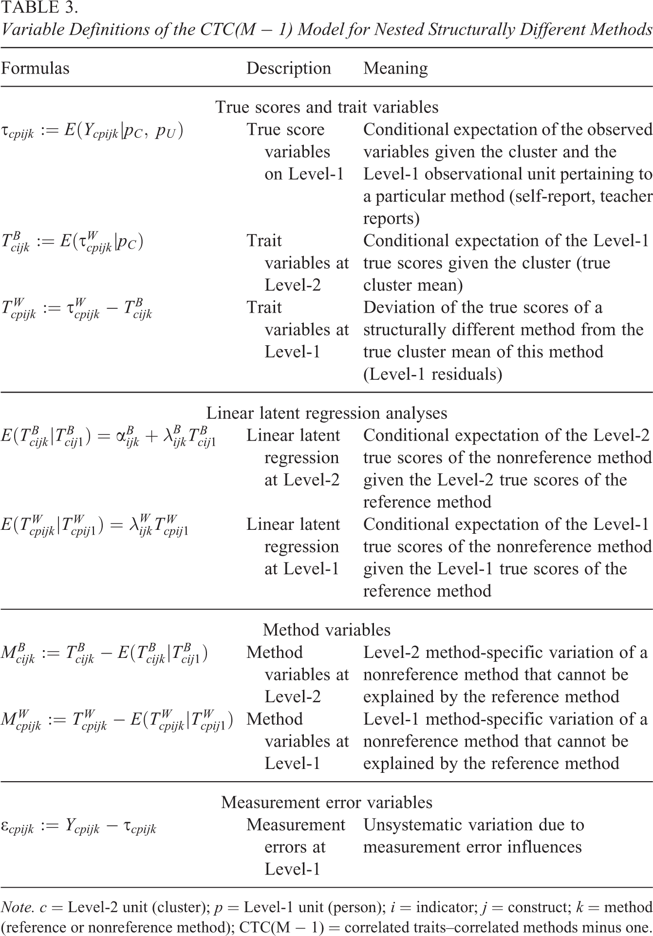
Note. c = Level-2 unit (cluster); p = Level-1 unit (person); i = indicator; j = construct; k = method (reference or nonreference method); CTC(M − 1) = correlated traits–correlated methods minus one.

A path diagram of the CTC(M − 1) model with indicator-specific latent trait factors on the within level (Level-1) and between level (Level-2) is depicted in Figure 3A. Figure 3B illustrates a more restrictive variant of the model with common latent trait factors. We generally recommend to test whether or not common (unidimensional) latent trait factors can be assumed by comparing the fit of both models (see Figure 3A and 3B).

Figure 3.
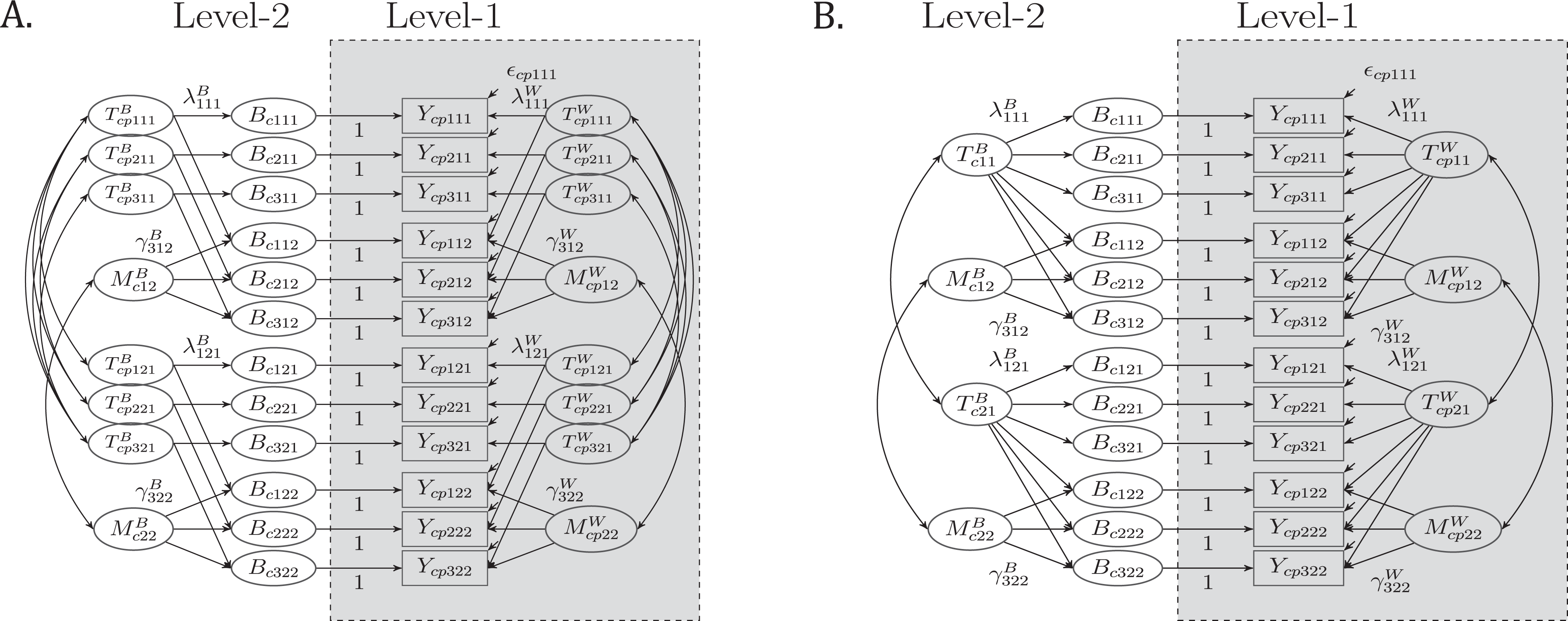
Path diagram of the multilevel, multiple indicator CTC(M − 1) model for nested structurally different methods with indicator-specific latent trait factors (see Figure 3A) and with unidimensional latent trait factors (see Figure 3B) for three indicators, two constructs, and two (structurally different) methods. Y_cpijk = observed variable on Level-1 p = person, c = cluster, i = indicator, j = construct, and k = method). $T_{c j 1}^{B}$ = unidimensional latent trait factor on Level 2. $T_{c p j 1}^{W}$ = unidimensional latent trait factor on Level 1. $M_{c j k}^{B}$ = unidimensional latent method factor on Level-2. $M_{c p j k}^{W}$ = unidimensional latent method factor on Level-1. ε_cijk = Level-1 error variable. $λ_{i j k}^{B}$ = Level-2 trait factor loading parameter. $λ_{i j k}^{W}$ = Level-1 trait factor loading parameter. $λ_{i j k}^{B}$ = Level-2 method factor loading parameter. $γ_{i j k}^{W}$ = Level-1 method factor loading parameter. Mean structure is not presented for clarity.

Empirical Application

Participants

For illustration purposes, we fit the new model to data from an educational research study investigating noncognitive characteristics in middle school students (N = 1,644; 50% males). The students’ age ranged from 10 to 15 years. Each student was rated by their class teacher (n = 217 teachers). In addition, students’ self-reports were collected. Due to privacy protections, students’ and teachers’ class membership (class ID) could not be assessed. Hence, it was impossible to account for additional clustering due to cross classification of teachers and classes. For the subsequent analysis, we used the teacher ID as cluster variable. On average, each teacher rated eight students.

Measures

For the assessment of intrinsic motivation and teamwork, short questionnaires were developed and matched for student and teacher ratings. Each short scale consists of 6 items, having a possible range of 1 (never or rarely) to 4 (usually or always). For each short scale, 2 item parcels were calculated as the mean of 3 items.

Statistical Analysis

The model as depicted in Figure 3B was fit to the data first. As can be seen from Figure 3B, we specified common latent trait and method factors at each level. Moreover, we restricted the factor loadings as well as error variances within each TMU to be equal, assuming τ-parallel test halves (parcels). Using this ML-CTC(M − 1) model, we calculated the variance coefficients using the model constraint option in Mplus (L. K. Muthén & Muthén, 1998–2012).

Results

The newly developed ML-CTC(M − 1) model with common trait and method factors fit the data well, χ²(50) = 129.24, p < .001, comparative fit index = .98, root mean square error of approximation = .03, standardized root mean square residual (SRMR_L1) = .01, SRMR_L2 = .06.

Table 4 provides information of the variance coefficients of reliability, intraclass correlation consistency, and method specificity. The results show that the reliability coefficients of student and teacher reports were acceptably high, ranging between .64 and .89. Interestingly, the reliability coefficients of the teacher reports were greater than those of the student reports. This indicates that both constructs were assessed with a greater accuracy (reliability) by teacher reports than by students’ self-reports. Moreover, the intraclass correlations (ICC) of the student reports were lower (.04) as compared to the ICCs of the teacher reports (.12–.15). This means that teacher ratings differed to a greater extent across clusters than student ratings. However, given that no class ID was included in the data set, these results should be interpreted with some caution.

Table 4.
ML-CTC(M − 1) Model With Unidimensional Latent Trait and Method Factors for Nested Structurally Different Methods: Reliability, Intraclass Correlation, Consistency, and Method Specificity at Level-1 and -2

Consistency Method Specificity

Rater Parcels Rel ICCs L1Con L2Con L1Msp L2Msp

Teamwork

Students Y_ce ₁₁₁ .64 .04 .63 1.00

Y_cp ₂₁₁ .64 .04 .63 1.00

Teachers Y_cp ₁₁₂ .85 .15 .06 .00 .77 1.00

Y_cp ₂₁₂ .85 .15 .06 .00 .77 1.00

Intrinsic Motivation

Students Y_cp ₁₂₁ .70 .04 .69 1.00

Y_cp ₂₂₁ .70 .04 .69 1.00

Teachers Y_cp ₁₂₂ .89 .12 .16 .10 .72 .90

Y_cp ₂₂₂ .89 .12 .16 .10 .72 .90

Note. Y_cpijk = observed variables; c = cluster (here teacher/class); p = person (here student); i = indicator (parcels); j = construct (1 = teamwork, 2 = intrinsic motivation); k = method (1 = student reports, 2 = teacher reports). Rel = reliability; ICC = intraclass correlation; L1Con = Level-1 consistency; L2Con = Level-2 consistency; L1Msp = Level-1 method specificity; L2Msp = Level-2 method specificity; ML-CTC(M − 1) = multilevel correlated traits–correlated methods minus one. The coefficients of consistency and method specificity were standardized on the observed variance of an indicator as defined in text.

The Level-1 consistency coefficients (L1-Con) pertaining to the teacher reports (i.e., nonreference method) was between .06 for teamwork and .16 for intrinsic motivation. This means that the convergent validity (i.e., square root of the consistency coefficients) between teacher and student reports at the individual level (Level-1) was higher for intrinsic motivation $(\sqrt{.16} = .40)$ than for teamwork $(\sqrt{.06} = .24)$ . In addition, the Level-2 consistency coefficients were consistently lower as compared to the Level-1 consistency coefficients. For teamwork, the Level-2 consistency coefficients were zero, revealing that students’ and teachers’ evaluations were uncorrelated at the cluster level (Level-2). This indicates that the degree in which teachers rated the students they assessed above the average of all students was not related to degree in which the aggregated self-rating of students was above or below the average of other groups of students, but rather a characteristic of the teachers themselves. For intrinsic motivation, the Level-2 consistency coefficients were .10, which indicates low convergent validity $(\sqrt{.10} = .32)$ between teacher and student reports at the cluster level.

The counterpart of the consistency coefficients is the method specificity coefficients. In this study, the Level-1 method specificity coefficients of the teacher reports ranged between .72 and .77, whereas the Level-2 method specificity coefficients were considerably higher (.90–1.00). The great amount of method specific variance at both levels suggests that teachers had a unique perspective on students’ noncognitive characteristics that was not shared with students’ self-reports.

In addition to the variance coefficients, we examined the correlations between the latent factors at both levels. The correlation between the latent trait factors can be interpreted as an indicator of discriminant validity. In this present study, the correlations between the latent trait factors were $r (T_{c p 11}^{W}, T_{c p 21}^{W}) = .58$ , p < .001 at Level-1 and $r (T_{p 11}^{B}, T_{p 21}^{B}) = .89$ , p < .001 at Level-2. These relatively high-positive correlations suggest that students did not differentiate extensively between intrinsic motivation and teamwork, but perceived both constructs as interrelated. The correlations between the latent method factors at both measurement levels can be interpreted as to which extent method effects generalized across constructs. The correlations between the latent method factors were $r (M_{c p 12}^{W}, M_{c p 22}^{W}) = .56$ , p < .001 at Level-1 and $r (M_{p 12}^{B}, M_{p 22}^{B}) = .70$ , p < .100 at Level-2. The results indicate that teachers tend to rate students’ abilities in a similar way regardless of which noncognitive characteristics (i.e., motivation or teamwork) they judged. The latent method correlations may be also interpreted as type of discriminant validity of the teacher reports corrected for students’ self-reports.

Overall, the results of this empirical application should be interpreted with great caution, given that there was no class ID included in the data set which allowed us to account for additional dependencies in the data. To examine the effects of sample size at Level-1 and Level-2, as well as the size of the ICC on the statistical performance of the ML-CTC(M − 1) model in greater detail, we report the results of a simulation study in the next section.

Simulation Study

To examine the statistical performance of the model depicted in Figure 3B, a Monte-Carlo simulation study was carried out. The main goal of the simulation study was to identify favorable and nonfavorable conditions, in which the model can be applied to real-life data and to determine the minimal required sample size for proper parameter estimates. For simplicity, a CTC(M − 1) model for nested structurally different methods with three indicators, two constructs, and two methods was chosen to ensure the minimal requirements of an MTMM-analysis (see Table 1). The simulation was done using Mplus 7.0 (L. K. Muthén & Muthén, 1998–2012) and the R package MplusAutomation (Hallquist, 2011). In total, 4 × 6 × 6 = 144 conditions with 500 replications per condition were simulated (72,000 data sets). All models were estimated using maximum likelihood (ML) estimator implemented in Mplus assuming complete data.

Simulation Design

Three important aspects of multilevel data were varied in this study: (a) the number of Level-1 units (nL1 = 5, 10, 15, 20, 30, and 40), (b) the number of Level-2 units (nL2 = 50, 100, 150, 200, 300, and 400), and (c) the intraclass correlation (ICC for the observed variables = low, medium, large, and extremely large). Results of previous simulation studies have shown that the number of Level-1 and -2 units and the level of intraclass correlation are important factors for proper parameter and standard errors (Hox & Maas, 2001; Julian, 2001; Koch, Schultze, Eid, et al., 2014). Hox and Maas (2001) showed that the number of Level-2 units are crucial for proper parameter estimates and recommended to sample at least 100 Level-2 units for multilevel SEM. In addition, previous findings indicated that the parameters on Level-2 are not trustworthy in conditions with few Level-2 units and low ICCs (Hox & Maas, 2001; Julian, 2001). Recent simulation studies in the field of multilevel MTMM modeling found that an increasing number of Level-1 units (cluster size) can decrease the amount of standard error bias (Koch, Schultze, Eid, et al., 2014). Based on these results, we choose four categories of ICCs: low (ICC ≈ .09–.10), medium (ICC ≈ .16–.19), large (ICC ≈ .25–.29), and extremely large (ICC ≈ .36–.69). According to Hox (2010) as well as Snijders and Bosker (2012), ICCs between .1 and .2 are common in educational studies, whereas greater ICCs (above. 3) are rather found in longitudinal or small group (multirater) studies.

The ICC coefficients were varied by choosing different population values of the standardized factor loadings and measurement error variances (see Equations 30 and 31). In Table 5, the population values of the standardized factor loading parameters and the error variances are presented. Given that previous application of CTC(M − 1) models indicating that the convergent validity (consistency) between structurally different methods are rather low, we decided to use higher method specificity coefficients (i.e., method factor loading values) in this study.

Table 5.
Population parameters used in the MC simulation study

Between (Level-2) Within (Level-1)

Method $λ_{i j k}^{B}$ $γ_{i j k}^{B}$ $λ_{i j k}^{W}$ $γ_{i j k}^{W}$ ${Var(∊}_{c p i j k}^{})$ ICC

RefMeth .30 – .90 – .10 .09

NonRefMeth .10 .30 .40 .80 .10 .10

RefMeth .40 – .85 – .1175 .16

NonRefMeth .15 .40 .35 .75 .1325 .1825

RefMeth .50 – .80 – .11 .25

NonRefMeth .20 .50 .30 .70 .13 .29

RefMeth .60 – .70 – .15 .36

NonRefMeth .30 .55 .25 .60 .1325 .3925

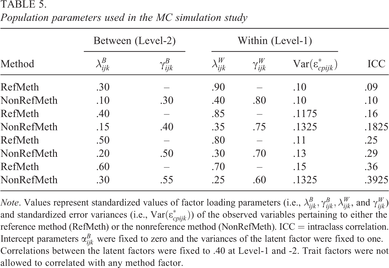
Note. Values represent standardized values of factor loading parameters (i.e., $λ_{i j k}^{B}, γ_{i j k}^{B}, λ_{i j k}^{W}$ , and $γ_{i j k}^{W}$ ) and standardized error variances (i.e., ${Var(∊}_{c p i j k}^{})$ ) of the observed variables pertaining to either the reference method (RefMeth) or the nonreference method (NonRefMeth). ICC = intraclass correlation. Intercept parameters $α_{i j k}^{B}$ were fixed to zero and the variances of the latent factor were fixed to one. Correlations between the latent factors were fixed to .40 at Level-1 and -2. Trait factors were not allowed to correlated with any method factor.

Estimation Bias

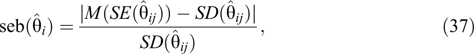
The statistical performance of the model was investigated with respect to two bias indices: parameter estimation bias (peb) and standard error bias (seb). The following formulas were used to calculate absolute peb and seb (cf. Holye, 2014):

$peb ({\hat{θ}}_{i}) = \frac{| M ({\hat{θ}}_{i j}) - θ_{i} |}{θ_{i}},$
36

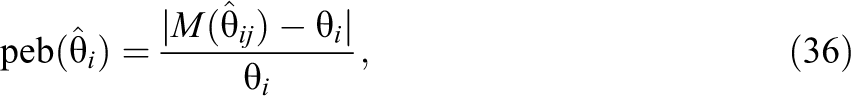
where θ _i is the true (population) value of the ith parameter and $M ({\hat{θ}}_{i j})$ is the average (mean) parameter estimate of the ith parameter across j (here: 500) MC replications. The absolute deviation of the estimate parameter estimation and population parameter were standardized with respect to the population parameter. Similarly, the relative standard error bias was calculated:

$seb ({\hat{θ}}_{i}) = \frac{| M (S E ({\hat{θ}}_{i j})) - S D ({\hat{θ}}_{i j}) |}{S D ({\hat{θ}}_{i j})},$
37

where $M (S E ({\hat{θ}}_{i j}))$ is the average estimated standard error for parameter i across j MC replications, and $S D ({\hat{θ}}_{i j})$ is the estimated population standard error for that parameter estimate (i.e., the standard deviation of the point estimate of parameter i across j replications).

The peb and seb coefficients for each parameter i were then averaged across the following parameter cluster for each level separately: (1) the within trait factor loadings (λ ^W ), (2) the between trait factor loadings (λ ^B ), (3) the within method factor loading (γ ^W ), (4) the between-method factor loadings (γ ^B ), (5) the within trait factor variances and covariances (ψ ^W ), (6) the between trait variances and covariances (ψ ^B ), (7) the within method factor variances and covariances (ϕ ^W ), (8) the between-method factor variances and covariances (ϕ ^B ), (9) the within residual variances (θ ^W ), and (10) the between intercept parameters (μ ^B ). A criterion of absolute bias below .10 (10%) was taken as the cutoff value for acceptable bias (Geiser, 2009; Eid et al., 2006; Koch, 2013; L. K. Muthén & Muthén, 2002).

Results

All models converged properly after a maximum of 100 ML iterations and 500 expectation–maximization iterations (default in Mplus). However, Mplus reported warnings concerning nonpositive latent variable covariance in 21 (.03%) of all 72,000 (i.e., 500 × 144) replications, ill-conditioned fisher information matrix in 2 (<.01%) out of all replications, problems computing standard errors in 2 (<.01%) $(< .01 %)$ out of all replications, and problems of reaching saddle points in the estimation process in 28 (.04%) out of all replications. All estimation problems occurred in conditions with low to medium ICCs and with just a minimal number of five Level-1 units per cluster. This indicates that CTC(M − 1) model for nested structurally different methods becomes slightly instable in extreme conditions with few Level-1 units (five per cluster) and low ICCs (ICC ≤ .10). Despite that the results seem rather encouraging given that the overall amount of estimation problems was negligible (below 5%) in this study.

In 3 (2.1%) of 144 MC conditions, the peb exceeded the cutoff value of .10. This was solely the case for Level-2 (between level) parameters such as trait and method factor loadings as well as latent correlations between the latent variables in the low ICC condition with five Level-1 units per cluster. Figure 4 illustrates the relationship between the level of ICC and the sample size on both levels for these model parameters. The maximum peb of .18 associated with a Level-2 method factor loading was encountered in the low ICC condition with 5 Level-1 and 50 Level-2 units.

Figure 4.
Peb for different levels of ICC (L = low, M = medium, H = high, and V = very high) and sample size on Level-1 (5, 10, 15, 20, 30, and 40) and Level-2 (50, 100, 150, 200, 300, and 400) for the Level-2 model parameters, L2lamMeth = method factor loadings (γ^B), L2corMeth = correlation between-method factors (ϕ^B), L2lamTrait = trait factor loadings (λ^B), and L2corTrait = correlation between trait factors (ψ^B). The dashed line represents the cutoff value of .10.

The standard errors of the parameter estimated exceeded the cutoff value of .10 in 14 (9.7%) of 144 MC conditions. Similar to the previous results, seb was especially large for Level-2 (between level) parameters in conditions with low ICCs and few observations per cluster (i.e., five Level-1 units). The maximum seb of 2.44 corresponding to the correlations of Level-2 method factors (i.e., generalizability of method effects) was again encountered in the low ICC condition with 5 Level-1 and 50 Level-2 units. Figure 5 depicts the absolute amount of seb for Level-1 and Level-2 parameters in relation to different ICC conditions as well as the number of Level-1 and Level-2 units. As Figure 5 shows the absolute seb of the Level-2 parameters (i.e., method factor loadings, correlation between-method factors, trait factor loadings, and correlation between trait factors) exceeded the cutoff value of .10 in condition with 5 Level-1 and 50, 100, and 150 Level-2 observations as well as in the condition with 10 Level-1 and 50 Level-2 observations. In the remaining conditions, the seb did not exceed the critical cutoff value .10.

Figure 5.
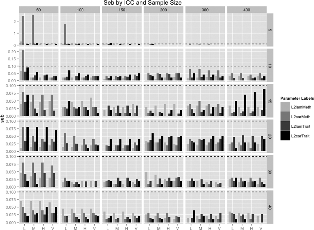
Seb for different levels of ICC (L = low, M = medium, H = high, and V = very high) and sample size on Level-1 (5, 10, 15, 20, 30, and 40) and Level-2 (50, 100, 150, 200, 300, and 400) for the Level-2 model parameters (L2lamMeth = methodfactor loadings (γ^B), L2corMeth = correlation between-method factors (ϕ^B), L2lamTrait = trait factor loadings (λ^B), and L2corTrait = correlation between trait factors (ψ^B). Note that the limits of the y-axis for the condition with five Level-1 units per cluster were rearranged to fit the figure. The dashed line represents the cutoff value of .10.

To combine the statistical properties of both point estimates and standard error estimates, we additionally report a coverage performance. In line with L. K. Muthén and Muthén (2002), we decided that coverage that remains between .91 and .98 is acceptable or tolerable. In 21 (14.6%) of 144 MC conditions, the coverage exceeded this range. Independent of the ICC, lower coverage was found in conditions with few Level-2 observations (100 or lower). Coverage above .98 were encountered in three cases of the MC condition with 150 Level-2 units and 5 Level-1 units per cluster. Moreover, poor coverage performance was exclusively associated with the estimation of Level-2 parameters. Overall, the maximum range of coverage was between .88 and .99 (M = .94, SD = .01).

To examine whether or not the different aspects of the data (i.e., number of Level-1 and Level-2 observations, level of ICC) have a significant impact on the trustworthiness of the parameter estimates and their standard errors, we performed analysis of variance (ANOVA). For the statistical analysis, we used the raw peb and seb values of each parameter to serve as dependent variables rather than the absolute values of peb and seb as expressed in Equations 21 and 22. The main reason for this was to obtain a normally distributed rather than of a right skewed dependent variable (i.e., raw peb and seb).

With regard to peb, ANOVA revealed that all aspects varied in this simulations study (i.e., level of ICC, number of observations on Level-1 and -2) were significantly associated with parameter bias. In particular, larger peb was significantly related to lower ICCs, F(3, 9,202) = 57.17, p < .001, η² = .017, and fewer Level-1, F(5, 9,202) = 47.45, p < .001, η² = .023, and Level-2 observations, F(5, 9,202) = 123.14, p < .001, η² = .060, but relatively low practical significance (η²).

With regard to seb, ANOVA revealed that the number of Level-1 units, F(5, 9,202) = 16.40, p < .001, η² = .009, and the number of Level-2 units, F(5, 9,202) = 4.21, p < .001, η² = .002, were the main determinants of seb. However, with regard to our simulation study, the level of ICC was not significantly related to seb, F(5, 9,202) = 1.83, p = .13, η² = .00, which is an interesting finding, given that multilevel models are generally recommended to avoid standard error bias if the ICC is greater than zero.

Discussion

Our goal in the present article was to extend the modeling framework proposed by Eid and colleagues (2008) to measurement designs of fully nested structurally different methods. It was argued that many MTMM measurement designs in educational, organizational, and social psychology research incorporate structurally different methods (e.g., self- and other reports) that are nested within higher cluster (classes or teams). In such cases, researchers should use multilevel, instead of single-level CTC(M − 1) models for structurally different methods.

There are three reasons for that. First, the multilevel CTC(M − 1) model enables researchers to model latent trait and method factors at both levels (within- and between-clusters) and thereby allow researchers to directly model the hierarchical nature of the data. Second, the model allows researchers to examine the convergent and discriminant validity of the given measures at both levels and calculate level-specific coefficients of consistency and method specificity. Third, by relating Level-1 and Level-2 covariates to the trait and method variables in the model, researchers are able to investigate potential causes of trait and method effects on both levels (within and between clusters).

Given that the model comprises the CTC(M − 1) modeling framework, it is possible to compare methods against a reference method that is not measured on the same scale/metric. For example, it would be possible to use different questionnaires in combination with physiological or objective measures within this framework. Moreover, the CTC(M − 1) model for nested structurally different method is defined with respect to a concrete random experiment. That means that the latent variables can be defined as random variables.

To illustrate and discuss the meaning of the ML-CTC(M − 1) model parameters, we presented the results of a real data application. The findings of the application revealed that students and teachers show higher agreement at the individual level (Level-1) than at the cluster level (Level-2). Moreover, greater teacher–student agreement was found for the evaluation of students’ intrinsic motivation than of students’ teamwork abilities. Despite some rater agreement, the major amount of variance of the teacher reports were not shared with students’ self-reports, and the discriminant validity was relatively low within and across clusters.

To examine the statistical performance of the model, we presented finding of an MC simulation study varying key determinants of multilevel data structures (i.e., sample size and the level of ICC). The results of the simulation study showed that parameter estimates were biased in conditions with low ICCs (<.10) and few observations at Level-1 (5 per cluster) and Level-2 (50 cluster). Level-2 (between level or cluster level) parameters were most sensitive to bias under such data constellations. These results suggest that the findings of the empirical application should be interpreted with care, although there were more than 200 clusters and more than five observations per cluster in the present application. Moreover, the findings of our simulation study are well in line with previous findings in the field of multilevel SEM (MSEM, Julian, 2001; Hox & Maas, 2001), showing that complex MSEMs require a minimal amount of dependency (clustering) in the data and enough Level-2 units.

In particular, our simulation study showed that the CTC(M − 1) model for nested structurally different methods becomes slightly instable in conditions with a low level of ICC (below .10) and few Level-1 (5 per cluster) and Level-2 (i.e., 50 cluster) observations. Therefore, we recommend to sample more than 10 Level-1 units and at least 50 Level-2 units when applying the model to real data. In data constellations of low level of ICC (below .10) and less than 50 Level-2 observations (clusters), we recommend specifying the original (single level) multiple indicator CTC(M − 1) model using adjustment techniques for the dependencies in the data.

It should be noted that in order to estimate the minimal required sample size, the complexity (e.g., number of parameters) of the model has to be taken into account. The models simulated in this study incorporated just two constructs measured by 3 items and two methods (i.e., 32 parameters on each level, in total 64 parameters). Presumably, a larger number of Level-2 and Level-1 units is needed for the estimation of more complex models with more than two traits and two methods. Nevertheless, the results of this simulation study are rather encouraging, showing that even complex multilevel CFA-MTMM models (e.g., CTCM − 1 model for nested structurally different methods with 64 parameter in total) perform acceptably well in terms of parameter and standard error bias in relatively small samples (e.g., 50 Level-2 × 15 Level-1 or 100 Level-2 × 10 Level-1 units). In cases of few Level-1 units per cluster (e.g., 5), it is recommended to sample at least 200 Level-2 units (i.e., clusters) in order to obtain proper parameter estimates and standard errors.

In case of few Level-1 and Level-2 units and low ICCs (below .10), researchers should be aware that Level-2 (between level or cluster level) parameters are likely to be biased. This becomes especially important whenever researchers seek to investigate the convergent and discriminant validity on Level-2 (i.e., cluster level). In particular, the factor loadings of the Level-2 trait and method factors as well as the standard errors of the correlations between trait and method factors will be biased under such conditions. However, according to our simulation study, the peb and seb can be significantly reduced by an increasing Level-1 and Level-2 observations. Alternatively, Bayesian estimation techniques may also be a possible solution for obtaining proper parameter estimates in data constellations with few observations and low ICC (see, e.g., Hox, van de Schoot, & Matthijsse, 2012; B. Muthén & Asparouhov, 2012). Interestingly, the standard error bias was not significantly associated with the level of ICC, when controlling for sample size at both levels.

Limitations and Future Research

Although the ML-CTC(M − 1) model is an extension of the single-level multiple indicator CTC(M − 1) model (Eid et al., 2003) to MTMM measurement designs with nested structurally different methods, it is limited in some aspects. First, the proposed model is defined for fully nested cross-sectional MTMM data sets. Current modeling approaches for cross-classified (Koch, Schultze, Minjeong, et al., 2014; Schultze et al., 2015) as well as longitudinal MTMM measurement designs (Courvoisier, Nussbeck, Eid, Geiser, & Cole, 2008; Geiser, Eid, Nussbeck, Courvoisier, & Cole, 2010; Koch, 2013; Koch, Schultze, Eid, & Geiser, 2014) need to be considered in future studies to broaden the area of applicability of the model. Second, the new model is defined for continuous observed variables. Thus, the results of the present simulation study cannot improvidently be generalized to cases in which (ordered) categorical observed variables are used. Third, more simulation studies are needed that focus on the robustness of the ML-CTC(M − 1) model. Although the results of the present simulation study showed that the ML-CTC(M − 1) performs surprisingly well under ideal data constellation (i.e., normality, no missing data, equal reliabilities, and equal number of continuous indicators per factor), it is not clear to what extent these findings can be transferred to less ideal data constellations (e.g., nonnormality, percentage of missingness, different numbers of indicators and different reliabilities, misspecification, and categorical data). We therefore encourage researchers to study the robustness of the new ML-CTC(M − 1) model in future simulation studies.

Formulas	Level	Meaning
Level-2 consistency
$L 2 Con (B_{c i j k}) = \frac{{(λ_{i j k}^{B})}^{2} Var (T_{c i j 1}^{B})}{Var (B_{c i j k})}$	Level-2	Proportion of true variance of a nonreference method indicator that is due to reference measured trait across clusters
Level-1 consistency
$L 1 Con (W_{c p i j k}) = \frac{{(λ_{i j k}^{W})}^{2} Var (T_{c p i j k}^{W})}{Var (W_{c p o j k})}$	Level-1	Proportion of true variance of a nonreference method indicator that is due to reference measured trait within clusters
Total consistency
$TC (Y_{c p i j k}) = L 2 Con (B_{c i j k}) + L 1 Con (W_{c p i j k})$
Level-2 method specificity
$L 2 Msp (B_{c i j k}) = \frac{(λ_{i j k}^{B}) Var (M_{c j k}^{B})}{Var (B_{c i j k})}$	Level-2	Proportion of true variance of a nonreference method indicator that is not due to reference measured trait, but due to method-specific influences across clusters
Level-1 method specificity
$L 1 Msp (W_{c p i j k}) = \frac{{(λ_{i j k}^{W})}^{2} Var (M_{c p j k}^{W})}{Var (W_{c p o j k})}$	Level-1	Proportion of true variance of a nonreference method indicator that is not due to reference measured trait, but due to method-specific influences within clusters
Total method specificity
$TMS (Y_{c p i j k}) = L 2 Msp (B_{c i j k}) + L 1 Msp (W_{c p i j k})$
Intraclass correlation coefficient
$ICC (Y_{c p i j k}) = \frac{Var (B_{c i j k})}{Var (B_{c i j k}) + Var (W_{c p i j k}) + Var (∊_{c p i j k})}$	for the observed variables
$ICC (τ_{c p i j k}) = \frac{Var (B_{c i j k})}{Var (B_{c i j k}) + Var (W_{c p i j k}) + Var (∊_{c p i j k})}$	for the true score variables
Reliability
$Rel (Y_{c p i j k}) = 1 - \frac{Var (∊_{c p i j k})}{Var (Y_{c p i j k})}$	Level-1	Ratio of true variance to observed variance

Formulas	Description	Meaning
True scores and trait variables
$τ_{c p i j k} : = E (Y_{c p i j k} \| p C, p U)$	True score variables on Level-1	Conditional expectation of the observed variables given the cluster and the Level-1 observational unit pertaining to a particular method (self-report, teacher reports)
$T_{c i j k}^{B} : = E (τ_{c p i j k}^{W} \| p_{C})$	Trait variables at Level-2	Conditional expectation of the Level-1 true scores given the cluster (true cluster mean)
$T_{c p i j k}^{W} : = τ_{c p i j k}^{W} - T_{c i j k}^{B}$	Trait variables at Level-1	Deviation of the true scores of a structurally different method from the true cluster mean of this method (Level-1 residuals)
Linear latent regression analyses
$E (T_{c i j k}^{B} \| T_{c i j 1}^{B}) = α_{i j k}^{B} + λ_{i j k}^{B} T_{c i j 1}^{B}$	Linear latent regression at Level-2	Conditional expectation of the Level-2 true scores of the nonreference method given the Level-2 true scores of the reference method
$E (T_{c p i j k}^{W} \| T_{c p i j 1}^{W}) = λ_{i j k}^{W} T_{c p i j 1}^{W}$	Linear latent regression at Level-1	Conditional expectation of the Level-1 true scores of the nonreference method given the Level-1 true scores of the reference method
Method variables
$M_{c i j k}^{B} : = T_{c i j k}^{B} - E (T_{c i j k}^{B} \| T_{c i j 1}^{B})$	Method variables at Level-2	Level-2 method-specific variation of a nonreference method that cannot be explained by the reference method
$M_{c p i j k}^{W} : = T_{c p i j k}^{W} - E (T_{c p i j k}^{W} \| T_{c p i j 1}^{W})$	Method variables at Level-1	Level-1 method-specific variation of a nonreference method that cannot be explained by the reference method
Measurement error variables
$∊_{c p i j k} : = Y_{c p i j k} - τ_{c p i j k}$	Measurement errors at Level-1	Unsystematic variation due to measurement error influences

				Consistency	Method Specificity
		Teamwork
Students	Y_ce ₁₁₁	.64	.04	.63	1.00
	Y_cp ₂₁₁	.64	.04	.63	1.00
Teachers	Y_cp ₁₁₂	.85	.15	.06	.00	.77	1.00
	Y_cp ₂₁₂	.85	.15	.06	.00	.77	1.00
		Intrinsic Motivation
Students	Y_cp ₁₂₁	.70	.04	.69	1.00
	Y_cp ₂₂₁	.70	.04	.69	1.00
Teachers	Y_cp ₁₂₂	.89	.12	.16	.10	.72	.90
	Y_cp ₂₂₂	.89	.12	.16	.10	.72	.90

	Between (Level-2)	Within (Level-1)
RefMeth	.30	–	.90	–	.10	.09
NonRefMeth	.10	.30	.40	.80	.10	.10
RefMeth	.40	–	.85	–	.1175	.16
NonRefMeth	.15	.40	.35	.75	.1325	.1825
RefMeth	.50	–	.80	–	.11	.25
NonRefMeth	.20	.50	.30	.70	.13	.29
RefMeth	.60	–	.70	–	.15	.36
NonRefMeth	.30	.55	.25	.60	.1325	.3925

Footnotes

Acknowledgement

The authors would like to thank Lisa Pullman, member institutions of the Elementary Schools Research Collaborative, and staff from the Center for Academic and Workforce Readiness of Success, Educational Testing Service for their support of this research.

Declaration of Conflicting Interests

The author(s) declared no potential conflicts of interest with respect to the research, authorship, and/or publication of this article.

Funding

The author(s) received no financial support for the research, authorship, and/or publication of this article.

Note

References

Brown

T. A.

(2012). Confirmatory factor analysis for applied research. New York, NY: Guilford Press.

Brownlie

E. B.

Lazare

Beitchman

(2012). Validating a self-report screen for adhd in early adulthood using childhood parent and teacher ratings. Journal of Attention Disorders, 16, 467–477.

Campbell

D. T.

Fiske

D. W.

(1959). Convergent and discriminant validation by the multitrait-multimethod matrix. Psychological Bulletin, 56, 81–105.

Carretero-Dios

Eid

Ruch

(2011). Analyzing multitrait-mulitmethod data with multilevel confirmatory factor analysis: An application to the validation of the state-trait cheerfulness inventory. Journal of Research in Personality, 45, 153–164.

Courvoisier

D. S.

Nussbeck

F. W.

Eid

Geiser

Cole

D. A.

(2008). Analyzing the convergent and discriminant validity of states and traits: Development and applications of multimethod latent state-trait models. Psychological Assessment, 20, 270–280.

Danay

Ziegler

(2011). Is there really a single factor of personality? A multirater approach to the apex of personality. Journal of Research in Personality, 45, 560–567.

Dumenci

(2000). Multitrait-multimethod analysis. In Brown

S. D.

Tinsley

H. E.

(Eds.), Handbook of applied multivariate statistics and mathematerial modeling (pp. 583–611). San Diego, CA: Academic Press.

Dunlop

Kornstein

Friedman

Rothschild

Pedersen

… Keller

(2010). Correlation between patient and clinician assessments of depression severity in the PREVENT study. Psychiatry Research, 177, 177–183.

Eid

(2000). A multitrait-multimethod model with minimal assumptions. Psychometrika, 65, 241–261.

10.

Eid

Lischetzke

Nussbeck

F. W.

Trierweiler

L. I.

(2003). Separating trait effects from trait-specific method effects in multitrait-multimethod models: A multiple-indicator CT-C(M-1) model. Psychological Methods, 8, 38–60.

11.

Eid

Nussbeck

F. W.

Geiser

Cole

D. A.

Gollwitzer

Lischetzke

(2008). Structural equation modeling of multitrait-multimethod data: Different models for different types of methods. Psychological Methods, 13, 230–253.

12.

Eid

Lischetzke

Nussbeck

F. W.

(2006). Structural equation models for multitrait-multimethod data. In Eid

Diener

(Eds.), Handbook of multimethod measurement in psychology (pp. 283–299). Washington, DC: American Psychological Association.

13.

Geiser

(2009). Multitrait-multimethod-multioccasion modeling. München, Germany: Akademischer Verlag München.

14.

Geiser

(2012). Data analysis with Mplus. New York, NY: Guilford Press.

15.

Geiser

Burns

G. L.

Servera

(2014). Testing for measurement invariance and latent mean differences across methods: Interesting incremental information from multitrait-multimethod studies. Frontiers in Psychology, 5, 1216.

16.

Geiser

Eid

Nussbeck

F. W.

(2008). On the meaning of the latent variables in the CT-C(M-1) model: A comment on Maydeu-Olivares and Coffman (2006). Psychological Methods, 13, 49–57.

17.

Geiser

Eid

Nussbeck

F. W.

Courvoisier

D. S.

Cole

D. A.

(2010). Analyzing true change in longitudinal multitrait-multimethod studies: Application of a multimethod change model to depression and anxiety in children. Developmental Psychology, 46, 29–45.

18.

Geiser

Eid

West

S. G.

Lischetzke

Nussbeck

F. W.

(2012). A comparison of method effects in two confirmatory factor models for structurally different methods. Structural Equation Modeling, 19, 409–436.

19.

Geiser

Koch

Eid

(2014). Data-generating mechanisms versus constructively defined latent variables in multitrait-multimethod analysis: A comment on Castro-Schilo, Widaman, and Grimm (2013). Structural Equation Modeling: A Multidisciplinary Journal, 21, 509–523.

20.

Hallquist

(2011). MplusAutomation: Automating Mplus model estimation and interpretation. Retrieved from http://cran.r-project.org/web/packages/MplusAutomation/index.html

21.

Hannum

K. M.

(2007). Measurement equivalence of 360-assessment data: Are different raters rating the same constructs? International Journal of Selection and Assessment, 15, 293–301.

22.

Hox

J. J.

(2010). Multilevel analysis techniques and applications (2nd ed.). New York, NY: Routledge.

23.

Hox

J. J.

Maas

C. J.

(2001). The accuracy of multilevel structural equation modeling with pseudobalanced groups and small samples. Structural Equation Modeling, 8, 157–174.

24.

Hox

J. J.

van de Schoot

Matthijsse

(2012). How few countries will do? comparative survey analysis from a Bayesian perspective. Survey Research Methods, 6, 87–93.

25.

Hoyle

R. H.

(2014). Handbook of structural equation modeling. New York, NY: Guilford Publications.

26.

Huber

P. J.

(1967). The behavior of maximum likelihood estimates under nonstandard conditions. Berkeley, CA: University of California Press.

27.

Höfling

Schermelleh-Engel

Moosbrugger

(2009). Analyzing multitrait-multimethod data. Methodology: European Journal of Research Methods for the Behavioral and Social Sciences, 5, 99–111.

28.

Julian

M. W.

(2001). The consequences of ignoring multilevel data structures in nonhierarchical covariance modeling. Structural Equation Modeling, 8, 325–352.

29.

Kenny

D. A.

(1976). An empirical application of confirmatory factor analysis to the multitrait-multimethod matrix. Journal of Experimental Social Psychology, 12, 247–252.

30.

Kenny

D. A.

Kashy

D. A.

(1992). Analysis of the multitrait-multimethod matrix by confirmatory factor analysis. Psychological Bulletin, 112, 165–172.

31.

Koch

(2013). Multilevel structural equation modeling of multitrait-multimethod-multioccasion data (Doctoral dissertation). Freie Universität Berlin, Germany.

32.

Koch

Eid

Lochner

(in press). Multitrait-multimethod-analysis: The psychometric foundation of CFA-MTMM models. In Irwing

Booth

Hughes

(Eds.), The Wiley handbook of psychometric testing. London, England: John Wiley.

33.

Koch

Schultze

Eid

Geiser

(2014). A longitudinal multilevel CFA-MTMM model for interchangeable and structurally different methods. Frontiers in Psychology, 5, 311.

34.

Koch

Schultze

Minjeong

Nussbeck

Praetorius

A.-K.

Eid

(2014). A multilevel CFA-MTMM model for structurally different and non-independent interchangeable methods. Manuscript submitted for publication.

35.

Little

T. D.

Jorgensen

T. D.

Lang

K. M.

Moore

E. W. G.

(2014). On the joys of missing data. Journal of Pediatric Psychology, 39, 151–162.

36.

Lüdtke

Marsh

Robitzsch

Trautwein

Asparouhov

Muthén

(2008). The multilevel latent covariate model: A new, more reliable approach to group-level effects in contextual studies. Psychological Methods, 13, 203–229.

37.

Marsh

H. W.

(1993). Multitrait-multimethod analyses: Inferring each trait-method combination with multiple indicators. Applied Measurement in Education, 6, 49–81.

38.

Marsh

H. W.

Bailey

(1991). Confirmatory factor analyses of multitrait-multimethod data: A comparison of alternative models. Applied Psychological Measurement, 15, 47–70.

39.

Marsh

H. W.

Grayson

(1995). Latent variable models of multitrait-multimethod data. In Hoyle

R. H.

(Ed.), Structural equation modeling: Concepts, issues, and applications (pp. 177–198). Thousand Oaks, CA: Sage.

40.

Marsh

H. W.

Hocevar

(1988). A new, more powerful approach to multitrait-multimethod analyses: Application of second-order confirmatory factor analysis. Journal of Applied Psychology, 73, 107–117.

41.

Muthén

B. O.

(1994). Multilevel covariance structure analysis. Sociological Methods & Research, 22, 376–398.

42.

Muthén

Asparouhov

(2012). Bayesian structural equation modeling: A more flexible representation of substantive theory. Psychological Methods, 17, 313–335.

43.

Muthén

L. K.

Muthén

B. O.

(1998–2012). Mplus user’s guide (7th ed.). Los Angeles, CA: Author.

44.

Muthén

L. K.

Muthén

B. O.

(2002). How to use a Monte Carlo study to decide on sample size and determine power. Structural Equation Modeling, 9, 599–620.

45.

Pohl

Steyer

(2010). Modeling common traits and method effects in multitrait-multimethod analysis. Multivariate Behavioral Research, 45, 45–72.

46.

Pohl

Steyer

Kraus

(2008). Modelling method effects as individual causal effects. Journal of the Royal Statistical Society: Series A (Statistics in Society), 171, 41–63.

47.

Satorra

Bentler

P. M.

(1994). Corrections to test statistics and standard errors in covariance structure analysis. In von Eye

Clogg

(Eds.), Latent variables analysis: Applications for developmental research (pp. 399–419). Thousand Oaks, CA: Sage.

48.

Satorra

Bentler

P. M.

(2001). A scaled difference chi-square test statistic for moment structure analysis. Psychometrika, 66, 507–514.

49.

Schermelleh-Engel

Keith

Moosbrugger

Hodapp

(2004). Decomposing person and occasion-specific effects: An extension of latent state-trait (LST) theory to hierarchical LST models. Psychological Methods, 9, 198.

50.

Schultze

Koch

Eid

(2015). The effects of non-independent rater sets in multilevel-multitrait-multimethod models. Structural Equation Modeling, 22, 439–448.

51.

Snijders

T. A. B.

Bosker

R. J.

(2012). Multilevel analysis: An introduction to basic and advanced multilevel modeling (2nd ed.). London, England: Sage.

52.

Uher

Farmer

Maier

Rietschel

Hauser

Marusic

… Aitchison

K. J.

(2008). Measuring depression: Comparison and integration of three scales in the GENDEP study. Psychological Medicine, 38, 289–300.

53.

White

(1980). A heteroskedasticity-consistent covariance matrix estimator and a direct test for heteroskedasticity. Econometrica, 48, 817–838.

54.

Widaman

K. F.

(1985). Hierarchically nested covariance structure models for multitrait-multimethod data. Applied Psychological Measurement, 9, 1–26.

55.

Williford

Fite

P. J.

Cooley

J. L.

(2015). Student–teacher congruence in reported rates of physical and relational victimization among elementary-school-age children: The moderating role of gender and age. Journal of School Violence, 14, 177–195.

56.

Wothke

(1995). Covariance components analysis of the multitrait-multimethod matrix. In Shrout

P. E.

Fiske

S. T.

(Eds.), Personality research, methods, and theory: A festschrift honoring Donald W. Fiske (pp. 125–144). Hillsdale, NJ: Lawrence Erlbaum.

				Consistency		Method Specificity
Rater	Parcels	Rel	ICCs	L1Con	L2Con	L1Msp	L2Msp
		Teamwork
Students	Y_ce ₁₁₁	.64	.04	.63	1.00
	Y_cp ₂₁₁	.64	.04	.63	1.00
Teachers	Y_cp ₁₁₂	.85	.15	.06	.00	.77	1.00
	Y_cp ₂₁₂	.85	.15	.06	.00	.77	1.00
		Intrinsic Motivation
Students	Y_cp ₁₂₁	.70	.04	.69	1.00
	Y_cp ₂₂₁	.70	.04	.69	1.00
Teachers	Y_cp ₁₂₂	.89	.12	.16	.10	.72	.90
	Y_cp ₂₂₂	.89	.12	.16	.10	.72	.90

	Between (Level-2)		Within (Level-1)
Method	$λ_{i j k}^{B}$	$γ_{i j k}^{B}$	$λ_{i j k}^{W}$	$γ_{i j k}^{W}$	${Var(∊}_{c p i j k}^{*})$	ICC
RefMeth	.30	–	.90	–	.10	.09
NonRefMeth	.10	.30	.40	.80	.10	.10
RefMeth	.40	–	.85	–	.1175	.16
NonRefMeth	.15	.40	.35	.75	.1325	.1825
RefMeth	.50	–	.80	–	.11	.25
NonRefMeth	.20	.50	.30	.70	.13	.29
RefMeth	.60	–	.70	–	.15	.36
NonRefMeth	.30	.55	.25	.60	.1325	.3925