Power to Detect Intervention Effects on Ensembles of Social Networks

Abstract

The hierarchical network model (HNM) is a framework introduced by Sweet, Thomas, and Junker for modeling interventions and other covariate effects on ensembles of social networks, such as what would be found in randomized controlled trials in education research. In this article, we develop calculations for the power to detect an intervention effect using the hierarchical latent space model, an important subfamily of HNMs. We derive basic convergence results and asymptotic bounds on power, showing that standard error for the treatment effect is inversely proportional to the product of the number of ties and the number of networks; a result rather different from the usual effect of cluster size in hierarchical linear models, for example. We explore these results with a simulation study and suggest a tentative approach to power for practical applications.

Keywords

asymptotics Bayesian statistics experimental design hierarchical latent space model hierarchical network model power sample size social network analysis

1. Introduction

Many large-scale educational interventions are applied to entire schools or entire grades within a school (e.g., Glennan & Resnick, 2004; Hord, Roussin, & Sommers, 2010; Matsumura, Garnier, & Resnick, 2010; McLaughlin & Talbert, 2006; Spillane, Correnti, & Junker, 2009) and target changes in the organizational structure or professional climate in the school. Social networks are an obvious outcome measure for interventions aimed at changing the social structure in the school since the network of relationships among teachers, administrators, and other school staff reveals not only how information or resources are shared but also the overall professional structure of the school: whether teachers are well connected, isolated into subgroups, completely isolated, and so on. For example, an intervention whose aim is to improve professional working relationships among school staff can be assessed through changes to the advice-seeking networks (Spillane et al., 2009). Interventions may also target student populations. An intervention aimed at reducing bullying and sexual aggression among adolescents (e.g., Espelage & Low, 2009) is likely to change the way students interact with each other, increasing the frequency of positive interactions and friendships.

Sweet, Thomas, and Junker (2013, 2014) introduced a modeling framework for estimating treatment effects for experiments on networks along with other network-covariate effects, and Sweet and Zheng (2014b) introduced a model that can capture network effects on network subgroup structure. These models have been used to help education researchers estimate the effects of being an English-language learner teacher on advice-seeking networks (Hopkins, Lowenhaupt, & Sweet, 2015), the effects of similarity in beliefs about teaching on advice-seeking ties (Spillane, Hopkins, & Sweet, 2015a), and the effects of teacher management style on peer subgroup structure (Sweet & Zheng, 2014a, 2014b). In addition, Sweet and Zheng (2015) examined the effects of network-level covariates on advice seeking; these included school/network size as well as indicators to compare advice seeking across subjects and years.

Despite the utility of modeling a network as an experimental outcome, virtually no work has been done to incorporate networks into experimental design where the network is the unit of randomization. This is surprising because the network is often the first observable outcome in large-scale studies involving individuals and their interactions. At a time in education research where null results are the norm (Coalition for Evidence-Based Policy, 2013), understanding the mechanisms and intermediate effects of interventions is crucial for furthering large-scale research.

Thus, if social networks are to be an outcome of any kind in a study, researchers need to know how many networks of what size are needed to detect effects. The purpose of this article is to initiate a body of research on experimental design for social networks, beginning with power analysis methodology for sample size calculations. Because of the complex dependence structure among ties in a social network, typical multilevel model power calculations are not applicable. We instead adapt some consistency and asymptotic normality results and use these results to construct analytical bounds for power.

The rest of the article is organized as follows: We begin by introducing some examples of networks in Section 2 and discuss how samples of networks can be modeled in Section 3. We focus on one type of network model, the hierarchical latent space model (HLSM) which we describe in Section 4 and discuss how this model can be specified for network-level interventions. In Section 5, we present two theorems that we use to construct power bounds. Finally, we assess our analytical results using a series of simulation studies presented in Section 6 and conclude by discussing practical applications and other extensions.

2. Some Motivating Examples

To motivate this work, let us begin with a few concrete examples. These examples will not only provide a context for our work on power but also frame this idea of a network as a unit of observation. Consider a social network of teachers in a school where the relationship is advice seeking, that is, a network tie is present from node i to node j if i goes to j for advice. Note that there are many relationships that could be measured among teachers: coteaching, collaboration, friendship, coparticipation in professional development, sharing of lesson plans, and so on. The types of networks further expand if we consider other types of individuals as well, but for our purposes, let us focus on this network of teachers in one school.

Thus, the teachers in this school make up one network, but a district includes many schools. Now consider the advice-seeking networks of teachers in all of these schools. One assumption made is that teachers do not have ties across schools. Granted, this may not be true in reality, but often we collect social network data within a single school at one time.¹ For relationships that tend to be face-to-face such as advice seeking or coteaching, this assumption is more valid.

Our example real-world data include 15 networks (schools) in one district in the United States (Pitts & Spillane, 2009). Figure 1 shows the 15 networks in 2007 and again in 2008, in the same order. The vertices represent the individuals, and the arrowed edges represent an advice-seeking relationship which point from the advice seeker to the advice provider. School staff members in each school were asked to nominate to whom they went for advice, and this information was collected in 2007 and 2008. Thus, we might be interested in comparing the networks in 2007 with the networks in 2008, and in this scenario, the network is the unit of observation.

Figure 1.

Advice-seeking networks from Pitts and Spillane (2009) collected in 2007 and 2008 show variability in network structure across schools and to some extent across years. Networks for each schools are shown in the same configuration across years.

Consider an alternative example in which schools (and the networks within them) are randomly assigned to participate in an intervention. Schools are often the unit of randomization in education research (Bloom, Richburg-Hayes, & Black, 2007; Raudenbush, 1997), so thinking about an entire school as the unit of observation is common. Let us also suppose that the intervention is hypothesized to affect how staff members interact with one another. We hypothesize that teachers in treated schools will collaborate with each other more often. Then we can examine collaboration networks to determine whether the treatment has been successful. Granted, education researchers are often interested in more than whether a large-scale intervention increases collaboration. The hypothesized theory of action is that increased collaboration improves teaching quality (and student achievement). In this scenario, the network then operates as an intermediate outcome; the intervention causes changes in the network which ultimately improves teacher and student outcomes.

Both of these examples involve comparing two samples of school networks where the network is the unit of observation such that we are interested in differences between the two groups of networks. But a network is made up of a collection of interdependent ties. In some ways, treating the network as the unit of observation is similar to observational studies or experiments on schools in which the school-level outcome (e.g., graduate rate) is based on units within the school (e.g., students). In education research, hierarchical linear models (HLMs) are the model of choice for accommodating the nesting of teachers within schools (Raudenbush & Bryk, 2002); the need for a multilevel models for modeling the network as an outcome is no different, and we introduce these models in the next section.

3. Hierarchical Network Models (HNMs)

Sweet et al. (2013) introduced a framework called HNMs to build multilevel models for samples of social networks to estimate for network-level effects. Their aim was to create a class of models that extended network models in a similar way that HLMs (Raudenbush & Bryk, 2002) extend the general linear model. Just as the cluster level is absent in a general linear model, the network level is absent in a single network model, which models only one network.

Sweet et al. (2013) introduced a framework called HNMs to build multilevel models for samples of social networks to estimate for network-level effects. Their aim was to create a class of models that extended network models in a similar way that HLMs (Raudenbush & Bryk, 2002) extends the general linear model. Just as the cluster level is absent in a general linear model, the network level is absent in a single network model, which models only one network.

HNMs then allow users to extend existing social network models for use with multiple, independent social networks. Rather than modeling a single network of teachers within a school, we now model several networks of teachers such that each network is bounded by school membership. Other examples include friendship networks within classrooms, peer networks within villages, dating networks within universities, and so on.

Thus, any multilevel extension of a single network model is considered an HNM, and all of these models can accommodate network-level covariates to estimate treatment effects. Sweet et al. (2013) introduced a multilevel extension of the latent space model (LSM; Hoff, Raftery, & Handcock, 2002), which we will describe in detail in Section 4, and Sweet et al. (2014) introduced several extensions of mixed membership stochastic blockmodels (Airoldi, Blei, Fienberg, & Xing, 2008). In addition, both Sweet et al. (2013) and Sweet et al. (2014) introduce models for interventions, and Sweet and Zheng (2015) explore network-level covariates more generally. Further, extensions of other social network models have been developed independently of the HNM framework, such as multilevel p ₂ models (Zijlstra, van Duijn, & Snijders, 2006). More importantly, education researchers are actually using these models. Spillane, Kim, and Frank (2012) used multilevel models to estimate covariate effects on teacher advice-seeking ties across schools, and Hopkins, Lowenhaupt, and Sweet (2015) used similar models to estimate the district-wide effect of being an English-language learner teacher on network connections.

3.1. Power Calculations for HLMs Are Not Applicable to HNMs

The issue however in designing experiments where the network is the unit of randomization is that researchers have little idea how many networks are needed to detect treatment effects. Moreover, typical power calculations for HLMs are not applicable to network models, and we illustrate this fact by reviewing power.

The power function for a hypothesis test φ is defined as $β_{φ} (θ) = E_{θ} [φ (X)]$ where X is the observed data and $θ \in Θ$ is the parameter in the hypothesis (Schervish, 1997). Generally, we consider the hypothesis test φ as having some rejection region R and test statistic T(X) and define the power function as $β (θ) = P (T (X) \in R | θ)$ (Casella & Berger, 2002).

For example, the level-α Wald test contrasting the hypotheses:

H_{0} : θ = θ_{0}

H_{1} : θ > θ_{0}

has a test statistic $T (X) = \hat{θ}$ and rejection region $R = {\hat{θ} : \hat{θ} > θ_{0} + Z_{α} S E (\hat{θ})}$ for a suitable cutoff Z _α. The power function is then $β (θ) = P (\hat{θ} > θ_{0} + Z_{α} S E (\hat{θ}) | θ)$ . The level of the test is β(θ₀), the probability of rejecting the null when the null is true. Thus, $S E (\hat{θ})$ inversely influences the power function.

To contrast power calculations for HNMs with HLMs, consider a model for a simple two-level randomized cluster trial with a balanced design, T clusters and s individuals per cluster given as:

Y_{i j} = θ_{0 j} + e_{i j} i = 1, \dots, s, j = 1, \dots, T,

θ_{0 j} = γ + θ W_{j} + u_{0 j},

where θ is the treatment effect and e_ij ∼ N(0, σ²) and u _0j ∼ N(0, τ²). Then $S E (\hat{θ})$ can easily be calculated and in fact,

S E {(\hat{θ})}^{2} = \frac{4 (τ + \frac{σ^{2}}{s})}{T} .

We use this example to highlight the HLM assumption that within-cluster residuals are independent. This assumption is unrealistic for HNMs because within-cluster (network) residuals are structured by the presence or absence of ties, which are rarely independent. For example, a friendship tie between A and B and between B and C is likely to affect the probability of a tie between A and C. Many current social network models accommodate dependence in a variety of ways (Frank & Strauss, 1986; Hoff et al., 2002; Snijders, Pattison, Robins, & Handcock, 2006). Therefore, power calculations for HNMs are not as straightforward as calculations for HLMs since we cannot assume independence among ties.

4. HLSMs

Although any HNM can be specified for estimating intervention effects, for the purposes of this article, we restrict our methods to a simple version of a single model, the HLSM (Sweet, Thomas, & Junker, 2013). We focus on this model for several reasons. The first is that the HLSM is one of the most common multilevel network models used education research. In addition, HLSMs are generally interpreted in ways similar to logistic regression which is familiar to education researchers. Finally, we want to begin with a simple intervention model where an intervention increases the likelihood of network ties and HLSMs can be specified in this way.

The HLSM is a multilevel extension of LSMs introduced by Hoff, Raftery, and Handcock (2002). There are two main assumptions of LSMs: First, each individual in the network occupies a position in a latent social space and the distance between any two individuals’ positions influences the probability of a tie between them. The second is that ties are independent conditional on the latent space positions. Additional assumptions of the HLSM are that the networks are independent and individuals in different networks do not share ties.

An example of an HLSM is given as:

\begin{array}{l} P (Y | β, ℤ) = \prod_{k} \prod_{i \neq j} P (Y_{i j k} | Z_{i k}, Z_{j k}, β_{k}, θ), \\ logit P [Y_{i j k} = 1 | β, Z_{k}] = β_{k} W_{i j k} - | Z_{i k} - Z_{j k} |, \\ β_{k} \sim MVN (μ_{β}, Σ_{β}), \\ Z_{i k} \sim M V N (μ_{Z}, Σ_{Z}), \end{array}

where Z_ik and Z_jk are the latent space positions for individuals i and j, respectively, in network k, and we see that the distance between these positions contributes negatively to the log-odds tie probability. Nodes far from one another in the latent space are less likely to have ties than nodes that are close.

In addition, β is a set of regression coefficients for covariates W_ijk which can include node-, dyad-, and network-level covariates along with an intercept term. Node-level covariates in social networks models either describe the node sending the tie W_ijk = W_ik or the node receiving the tie W_ijk = W_jk . For example, the number of years of teaching experience is a covariate that can be associated with sending ties and receiving ties; if we consider advice seeking, experienced teachers may not be more likely to seek advice but may be much more likely to provide advice. Dyad-level covariates are variables determined by a pair of nodes; these include binary variables such as whether two nodes are the same race or gender as well as quantitative variables measuring differences in experience, hours of training, and so on.

Network-level covariates W_ijk = W_k are those attributes that describe the network. For example, we may include network size in the HLSM since networks of different sizes tend to have different densities (proportion of observed ties). Other covariates are likely context-specific; for example, with friendship networks within schools, we might be interested in school achievement or school socioeconomic status as predictors. In the context of an intervention, a binary treatment indicator could be used to estimate the effects of the experiment on network density. Another way to specify an HLSM is to include network-level covariates as part of the intercept term which is how HLMs often specify level-2 variables. We could then add $μ_{β 0} = γ_{0} + θ X_{k}$ to Equation 2 or if we assume zero covariance for β, we would write $β_{0 k} \sim N (γ_{0} + θ X_{k}, σ^{2})$ .

Network-level covariates W_ijk = W_k are those attributes that describe the network. For example, we may include network size in the HLSM since networks of different sizes tend to have different densities (proportion of observed ties). Other covariates are likely context-specific; for example, with friendship networks within schools, we might be interested in school achievement or school socioeconomic status as predictors. In the context of an intervention, a binary treatment indicator could be used to estimate the effects of the experiment on network density. Another way to specify an HLSM is to include network-level covariates as part of the intercept term which is how HLMs often specify level-2 variables. We could then add $μ_{β 0} = γ_{0} + θ X_{k}$ to Equation 2 or if we assume zero covariance for β, we could write $β_{0 k} \sim N (γ_{0} + θ X_{k}, σ^{2})$ .

If we include a treatment indicator as part of the intercept term, we assume that the treatment will affect overall tie probability. That is with a positive treatment effect, treated networks will have higher tie probability than control networks, conditional on other parameters in the model. Another way to model the same phenomenon is to include the treatment effect in the variance of the latent space positions; treated networks will have smaller variance (and overall closer latent space positions resulting in higher tie probabilities). There are other ways to specify interventions using HLSMs as well. An intervention could impact the effects of another covariate, so that the treatment effect would be part of an interaction term. Similarly, the treatment may only affect ties between certain types of individuals.

Consider our advice-seeking networks presented in Section 2. We can use an HLSM to compare the 2007 networks with the 2008 networks. In fact, as part of a chapter on incorporating network-level covariates into HLSMs, Sweet and Zheng (2015) fit an HLSM to compare these two groups of networks. They fit the following HLSM,

\begin{array}{l} P (Y | β, θ, ℤ) = \prod_{k} \prod_{i \neq j} P (Y_{i j k} | Z_{i k}, Z_{j k}, β_{k}, θ), \\ logit P [Y_{i j k} = 1 | β, θ, Z_{k}] = β_{0} + θ X_{k} + | Z_{i k} - Z_{j k} |, \\ β_{0} \sim N (μ_{0}, σ_{0}), \\ θ \sim N (μ_{θ}, τ_{θ}), \\ Z_{i k} \sim MVN (μ_{Z}, Σ_{Z}), \end{array}

where X_k is an indicator variable for being a 2007 network.

We present this example for several reasons. First to motivate this article on power. In this example, the authors did find a very small negative effect. The reported expected a posteriori estimate for θ is −0.22 with a posterior standard deviation of 0.09 which, for all intents and purposes, is significant but just barely. If one school was missing or if the schools were slightly smaller, would such an effect be detectable?

The second reason is to illuminate model estimation issues because LSMs (and HLSMs) pose an interesting estimation problems; there are constraints needed for the model to be identified. Estimating latent positions requires a constraint discussed in detail in Hoff et al. (2002) and Sweet et al. (2013). Here the issue is the identifiability issue between estimating the network intercept β₀ and the variance of the latent space positions Σ _Z . For example, low tie probability results from a small intercept but also from latent space positions with a large variance.

The confounding between intercept value and latent space distance is especially problematic when estimating an HLSM. Thus, fitting models with random intercepts is the same as fitting models with fixed intercepts since the average pairwise distance among latent space positions varies across networks. Because the latent positions are estimated and because the pairwise distance of these positions as well as an intercept term contributes to tie probability, fixed-intercept models are essentially the same as random-intercept models without strong priors or constraints on both β₀ and Σ _Z . Thus, what we find in practice is that random intercepts in HLSMs do not operate in the same way as random intercepts in HLMs and we want to make that explicit to readers.

For this article, we will focus on HLSMs where β_0k = β₀. This constraint along with a loose constraint on the upper bound on the latent space pairwise distance mediates the identifiability issue as well as improves intercept parameter recovery. We caution the reader however that models in which β₀ is the same across networks does not imply that tie probability is the same across all networks.

5. Sample Size Calculations for the HLSM

Power calculations hinge on an accurate estimate of the intervention effect standard error. Because the HNM dependence structure differs from classical HLM dependence, standard error calculations for HLMs are not applicable. We instead develop bounds for treatment effect standard error from first principles.

5.1. Standard Error of Treatment Effect

Consider an experiment on a collection of networks. In a typical experiment, some networks receive the treatment and the remainder are considered control networks. For example, if each network is a school, we might randomly assign schools to be in the treatment or control arms of our experiment and we assume the schools to be independent in that the outcome of one school is not influenced or dependent on the outcome of another school. We also recognize that school networks are not identical in size, structure, or functionality, and our statistical models reflect that. In the HNM framework, we model these networks to be independent of one another but not identically distributed.

Note that consistency of maximum likelihood estimates (MLEs) when observations are independently and identically distributed is well documented (Casella & Berger, 2002). Given independent but not identically distributed data, Cramér (1946) proved that the MLE is both consistent and asymptotically normal. We adapt his work along with other adaptations of Chanda (1954) and Bradley and Gart (1962) to show that the posterior mode estimator for a treatment effect in Equation 2 is both consistent and asymptotically normal. We then use the asymptotic distribution for this parameter to estimate its standard error and compute power.

Our development is organized into two main collections of results. Only the final results appear below as two theorems. The first states that the posterior mode of any network-level covariate is consistent, and the second concludes that the posterior mode asymptotically follows a normal distribution. While this result is familiar, and helpful in establishing standard inferential procedures, it is also surprising, given the complex dependence structure in each network.

The proofs of the theorems appear in detail in the Online Appendix. These results are not trivial; rather, they are the culmination of a series of results. For each theorem, we first establish the result conditional on the latent space positions $ℤ$ . Note that conditioning on $ℤ$ does not mean that our latent space positions are known or fixed; they remain latent parameters, but rather that we are conditioning on the unknown values of these positions for our proof. Once we have proved each result conditional on the $ℤ$ , we remove this condition in the theorem. Note also that these results hold for any network-level covariate effect in an HLSM as in Equation 2 as well as for a binary covariate such as in Equation 3.

Theorem 5.1: (Consistency of the Posterior Mode, Unconditional on the Latent Space Positions)

Define our HLSM as:

logit [P (Y_{i j k} = 1)] = β_{k} W_{i j k} + θ X_{k} - d_{i j k}, i, j = 1, \dots, m_{k},

where W_ijk are a collection of covariates and d_ijk = |Z_ik − Z_jk |. Let θ be a network-level covariate and $\hat{θ}$ be posterior mode where θ₀ is the true effect. Let m_k be the number of nodes in network k such that $_{n→∞}^{\lim} max (m_{1},. . ., m_{n}) < \infty$ . Then, unconditional on the latent space positions, $\hat{θ}$ is consistent: $P (| \hat{θ} - θ_{0} | > ε) \to 0$ as $n \to \infty$ .

Theorem 5.2: Asymptotic Normality of the Posterior Mode, Unconditional on the Latent Space Positions

Let θ be the network-level covariate effect in the HLSM given in Equation 4 with posterior mode $\hat{θ}$ and true effect θ₀. Then unconditional on the latent space positions, $\hat{θ}$ is asymptotically normal, that is,

$\sqrt{\sum_{k = 1}^{n} C_{k}^{2}} (\hat{θ} - θ_{0}) \overset{D}{\to} N (0, 1)$ , where $C_{k}^{2}$ is the Fisher Information of θ for network k. For the HLSM defined in Equation 4, $C_{k}^{2} = E [\sum_{i, j = 1 i \neq j}^{m_{k}} \frac{X_{k}^{2} \exp (β_{k} W_{i j k} + θ_{0} X_{k} - d_{i j k})}{{(1 + \exp (β_{k} W_{i j k} + θ_{0} X_{k} - d_{i j k}))}^{2}}]$ .

Given the asymptotic distribution of $\hat{θ}$ proved in Theorem 5.2, $\hat{θ} \overset{D}{\to} N (θ_{0}, \frac{1}{\sum_{k = 1}^{n} C_{k}^{2}})$ , we can use $\sqrt{\frac{1}{\sum_{k = 1}^{n} C_{k}^{2}}}$ as an estimate for $S E (\hat{θ})$ . Recall also that $\sum_{k = 1}^{n} C_{k}^{2}$ is a function of the latent space positions which are not known a priori. Instead, we find reasonable bounds for $\sum_{k = 1}^{n} C_{k}^{2}$ , taking advantage of the log-odds ratio structure of the HLSM.

Thus, given that

\sum_{k = 1}^{n} C_{k}^{2} = \sum_{k = 1}^{n} \sum_{i, j}^{m_{k}} [\frac{X_{k}^{2} \exp (β_{k} W_{i j k} + θ X_{k} - d_{i j k})}{{(1 + \exp (β_{k} W_{i j k} + θ X_{k} - d_{i j k}))}^{2}}],

suppose there is constant network size m. We can easily construct an upper bound for $\sum_{k = 1}^{n} C_{k}^{2}$ since $\frac{X_{k}^{2} \exp (β_{k} W_{i j k} + θ X_{k} - d_{i j k})}{{(1 + \exp (β_{k} W_{i j k} + θ X_{k} - d_{i j k}))}^{2}}$ has a maximum possible value of $\frac{1}{4}$ for any value of $X_{k} \in {0, 1}$ , $θ \in ℝ$ , and $d_{i j k} \in ℝ$ . Therefore,

\sum_{k = 1}^{n} C_{k}^{2} \leq \frac{m n (m - 1)}{4},

where m is the number of nodes or members per network and n is the number of networks.

For a lower bound, if we assume $| β_{k} W_{i j k} + θ - d_{i j k} | \leq a$ , then $\frac{\exp (β_{k} W_{i j k} + θ - d_{i j k})}{{(1 + \exp (β_{k} W_{i j k} + θ - d_{i j k}))}^{2}} \geq \frac{\exp (a)}{{(1 + \exp (a))}^{2}}$ , for all values $| β_{k} W_{i j k} + θ - d_{i j k} | < a$ . And in fact, $\frac{\exp (β_{k} W_{i j k} + θ - d_{i j k})}{{(1 + \exp (β_{k} W_{i j k} + θ - d_{i j k}))}^{2}}$ asymptotically approaches 0 as $| β_{k} W_{i j k} + θ - d_{i j k} | \to \infty$ . Figure 2 illustrates this relationship.

Figure 2.

Relationship between $\frac{\exp (θ - d_{i j k})}{{(1 + \exp (θ - d_{i j k}))}^{2}}$ and $θ - d_{i j k}$ .

In the context of an experiment, X_k is a binary variable, so let X_k = 1 indicate a treated network. We then define f be a lower bound on the proportion of treated networks, so that

\sum_{k = 1}^{n} C_{k}^{2} = \sum_{k = 1}^{n} \sum_{i, j}^{m} [\frac{X_{k}^{2} \exp (β_{k} W_{i j k} + θ X_{k} - d_{i j k})}{{(1 + \exp (β_{k} W_{i j k} + θ X_{k} - d_{i j k}))}^{2}}] \geq \frac{f n m (m - 1) \exp (a)}{{(1 + \exp (a))}^{2}} .

Therefore, we have the following bounds:

\frac{f n m (m - 1) e^{a}}{{(1 + e^{a})}^{2}} \leq \sum_{k = 1}^{n} C_{k}^{2} \leq \frac{n m (m - 1)}{4},

and since $Var (θ) = \frac{1}{\sum_{k = 1}^{n} C_{k}^{2}}$ by Theorem 5.2,

\frac{4}{n m (m - 1)} \leq V a r (\hat{θ}) \leq \frac{{(1 + e^{a})}^{2}}{f n m (m - 1) e^{a}}

\sqrt{\frac{4}{n m (m - 1)}} \leq S E (\hat{θ}) \leq \sqrt{\frac{{(1 + e^{a})}^{2}}{f n m (m - 1) e^{a}}} .

From Equation 5, it appears that the number of networks n and the number of ties m(m − 1) drive standard error equally, but we also have a parameter a that must be specified by the user. As we will see in Section 5.2.1, the value of a tends to increase as the number of nodes m increases, so the relationships between n and power and m(m − 1) and power may not be exactly equal.

5.2. Constructing Power Bounds

Given the bounds for $S E (\hat{θ})$ in Equation 5, we can easily construct upper and lower bounds for power, assuming we have selected f and a. We now discuss methods for selecting a and f as well as calculate bounds for experiments involving networks of various size and intervention effect.

Recall that f is a lower bound on the proportion of treated networks. Since an experiment hinges on having treated subjects, f > 0 and typically $f = \frac{1}{2}$ . Choosing a is more complicated since a is defined as:

| β_{k} W_{i j k} + θ - d_{i j k} | \leq a .

Note that $| β_{k} W_{i j k} + θ - d_{i j k} |$ corresponds to the linear component of the HLSM. That is, the probability of a tie from i to j is falls in the interval $[\frac{\exp (- a)}{1 + \exp (- a)}, \frac{\exp (a)}{1 + \exp (a)}]$ , so by choosing a value for a, we are choosing the range of tie probabilities. Taking advantage of the logit structure of the HLSM, a large value of a increases the range of probabilities only slightly more than a moderately large value of a, but large differences in a result in large differences in power estimates as we will later demonstrate.

To provide a context, we compute the ranges of tie probabilities when a = 4, a = 5, and a = 6 (see Table 1). Note that a represents the range of possible tie probabilities in the HLSM in general and is not impacted by the value of the θ.

Table 1.

The Interval of Tie Probabilities Specified by the Choice of a

Probability Bounds	a
[0.018, 0.982]	4
[0.007, 0.993]	5
[0.002, 0.997]	6

5.2.1. Empirically calculating a

To determine how a varies with network size in practice, we use simulated data to empirically estimate a. For various combinations of numbers of networks and numbers of nodes, we generated 100 data sets from an HLSM without covariates with an expected tie probability of 0.25. Within each replication and for each network, we examined the absolute probabilities of each tie and used the 99th quantile as the bound for that network. We then used the mean bound across all n networks and 100 replications for an empirical estimate of a. Thus, $\hat{a} = \frac{1}{100} \sum_{s = 1}^{100} \frac{1}{n} \sum_{k = 1}^{n} a_{k s}^{⋆}$ where $a_{k s}^{⋆} = {| β_{0} + θ X_{k} - d_{i j k} |}_{0.99}$ for all i, j in network k.

Table 2 illustrates the relationship between network size (number of nodes in the network) and a. Empirical estimates of a range between 4 and 5 but appear to increase systematically as network size increases which suggests that the number of nodes within each network is related to a. This is unsurprising since increased network size results in a quadratic increase in the number of ties and the potential for extreme tie probabilities increases. Still, these estimates suggest that a = 4, 5, 6 are plausible values for a under these conditions.

Table 2.

Empirical Estimate for the Size of a, the Bound on the Tie Probability, Calculated From Simulated Data

n	Network of Size 10	Network of Size 15	Network of Size 20
6	4.43	4.73	4.96
10	4.38	4.71	4.96
20	4.38	4.74	4.97
30	4.37	4.77	4.94
40	4.34	4.74	4.94
50	4.35	4.75	4.95

Thus, we use all three values for comparison as we construct our power intervals, which we calculate using the following formula.

Power_{UB} = P_{H_{1}} (\hat{θ} > θ_{NULL} + Z_{\frac{α}{2}} S E {(\hat{θ})}_{LB}),

Power_{LB} = P_{H_{1}} (\hat{θ} > θ_{NULL} + Z_{\frac{α}{2}} S E {(\hat{θ})}_{UB})

Assuming θ_NULL = 0 (i.e., no treatment effect), Table 3 provides examples of lower bounds for power for various combinations of numbers of network sizes (m), number of networks in the experiment (n), two different alternative hypotheses (θ = 0.75 and θ = 0.5), and our three values of a. Table 3 only includes lower bounds since the upper bound is ≈1 for all cells.

Table 3.

Examples of Power Lower Bounds

		Power	Lower	Bound
Treatment Effect	(m, n)	a = 6	a = 5	a = 4
θ = 0.5	(10, 10)	0.07	0.13	0.28
	(10, 20)	0.10	0.22	0.50
	(15, 10)	0.12	0.25	0.56
	(15, 20)	0.19	0.44	0.85
θ = 0.75	(10, 10)	0.11	0.24	0.55
	(10, 20)	0.19	0.43	0.84
	(15, 10)	0.21	0.49	0.89
	(15, 20)	0.38	0.79	0.99

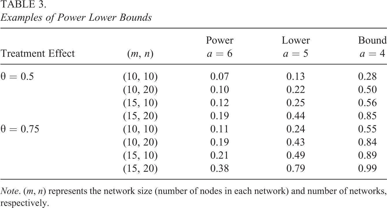
Note. (m, n) represents the network size (number of nodes in each network) and number of networks, respectively.

The upper bound is generally close to 1 because the lower bound for standard error $\frac{4}{n m (m - 1)}$ is quite small even for moderate sizes of m and n. Thus, the upper bound is not useful from a practical standpoint but provides a place for improvement in future methodological research. For sample size calculations, however, a lower bound is more important since power calculations are generally used to determine the minimum sample size needed to achieve specific power.

As expected, decreasing effect size decreases power and increasing the number of networks increases power. Recall that network size is also equally related to power (for a given value of a) and increasing the network size from 10 to 15 individuals greatly increases power. Note also that network size and number of networks both contribute in asymptotically driving $S E (\hat{θ})$ to zero, see Equation 5. This relationship is not true in a typical HLM power calculation (see Equation 1), since cluster size m does not drive the standard error to zero. By the same token, we have empirical evidence that a increases as m increases, but the exact relationship between m and a is unclear.

6. Simulations

We conduct a series of simulations, both to assess the analytical power bound results derived in Section 5 and to understand how these bounds can be used in practice. We first examine the distribution of the treatment effect estimator, since our results assume asymptotical normality of this estimator. Then, we compare empirical power estimates with the analytical lower bound. Regarding practical use, our primary goal is to further illuminate the relationship between power, network size, number of networks, and how a varies empirically as well.

The simulation study involved a combination of two treatment effects, three network sizes, and six different total numbers of networks. We specifically chose treatment effects, network sizes, and numbers of networks to cover a wide range of power estimates while focusing on network sizes that could be found in schools or classrooms. We assumed equal numbers of treated and untreated networks. The full design is given in Table 4.

Table 4.

Simulation Design

Treatment Effect	Network Size (m)	Number of Networks (n)
Treatment Effect	Network Size (m)	6	10	20	30	40	50
θ = 0.5
	10	x	x	x	x	x	x
	15	x	x	x	x	x	x
	20	x	x	x	x	x	x
θ = 0.75
	10	x	x	x	x	x	x
	15	x	x	x	x	x	x
	20	x	x	x	x	x	x

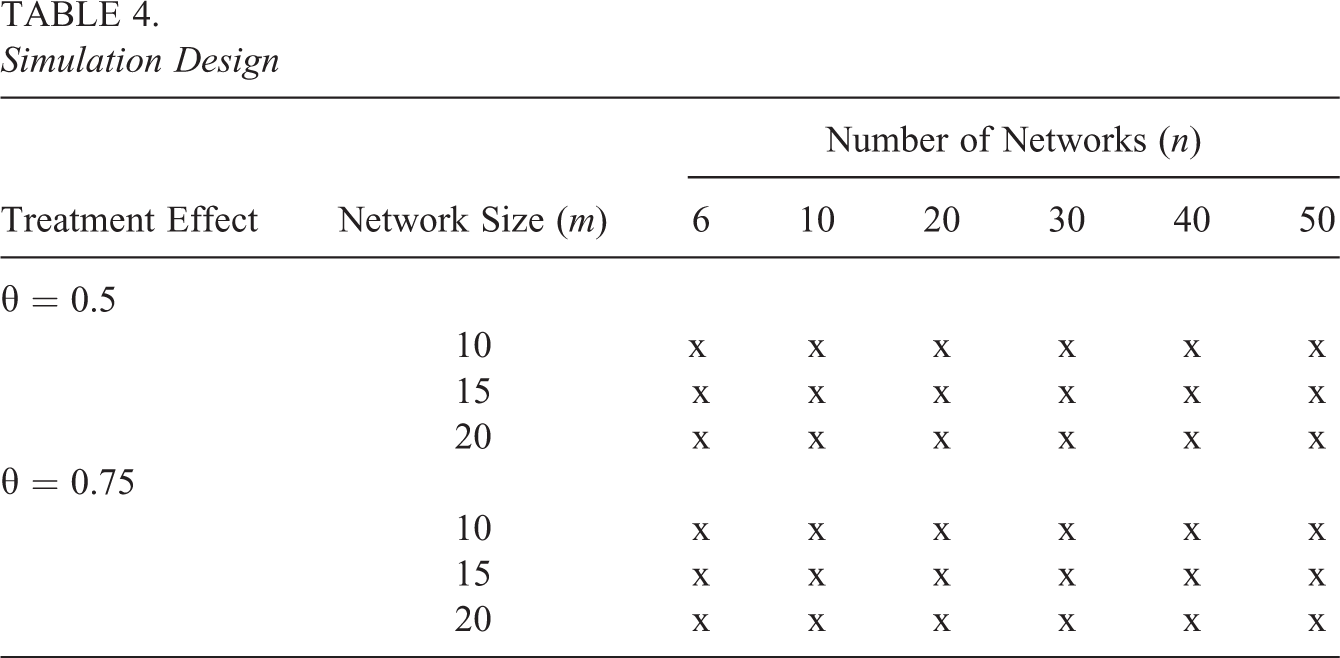
For each cell in Table 4, we simulated 100 data sets from the generative model.

\begin{array}{l} logit P [Y_{i j k} = 1] = 1.5 + θ T_{k} + | Z_{i k} - Z_{j k} | \\ Z_{i k} \sim M V N ((\begin{matrix} 0 \\ 0 \end{matrix}), (\begin{matrix} 3 & 0 \\ 0 & 3 \end{matrix})), i = 1, . . ., m, k = 1, . . ., n, \end{array}

where the intercept 1.5 was chosen to produce tie probabilities averaging near 0.25. Note that using the same value for β₀ does not imply that the mean tie probability is the same across networks. Recall network variability results from using different values of β₀ as well as from latent space positions, so there is some variability across networks in terms of tie probability. Admittedly, our aim was to keep the variability small which, depending on the context, may not be realistic, and additional work on the relationship between latent space/network tie probability variability and power is needed.

For each data set, we fit a similar HLSM to Equation 8 to the simulated data with uninformative priors, θ ∼ N(0, 100), β₀ ∼ N(0, 100), and latent space prior variance of 20I, using a Markov chain Monte Carlo algorithm coded in R (Sweet et al., 2013). For each model fit, we discarded the first 1,000 samples and retained every 25th draw from our remaining 9,000 samples for a θ posterior sample of 360.

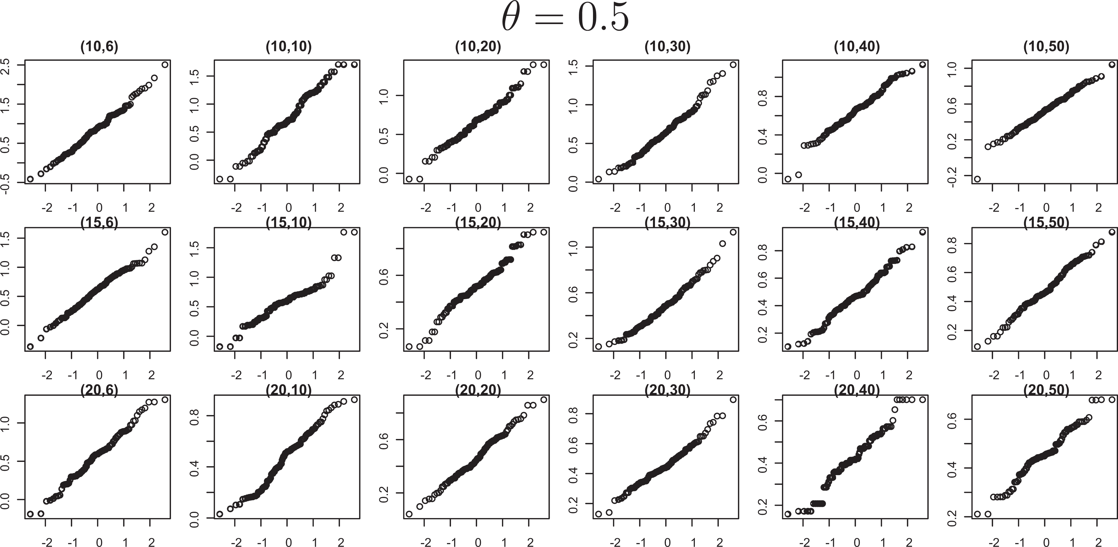
Because our power calculations are based on the asymptotic normal distribution of the posterior mode $\hat{θ}$ , we also compare the distribution of the 100 posterior modes to that of a normal distribution. Visual inspection of quantile-quantile plots suggests that posterior modes are approximately normal (Figure 3).

Figure 3.

Quantile-quantile plots for posterior modes suggest normality.

To evaluate our power lower bound formula, we compare our lower bound estimates with empirical power estimates. For each combination of (θ, m, n) shown in Table 4, we estimated power by taking the proportion of trials with detectable treatment effects, that is, the 95% equal–tailed credible interval for θ did not include 0.

Table 5 compares the relationship between the calculated lower bounds calculated using a = 4, a = 5, a = 6, and simulated power estimates. Regardless of treatment effect, increasing the number or size of networks generally increases power, and the larger treatment effect generates larger power estimates, as predicted by our formulas in Equations 5 and 7, respectively. We also include an estimate for level, that is, when the true treatment effect is 0.

Table 5.

Empirical Estimates for Power Are Similar to Analytical Power Lower Bounds

		θ = 0.5				θ = 0.75
Treatment	θ = 0 Level	Lower Bound			Power	Lower Bound			Power
(m, n)	Est.	a = 6	a = 5	a = 4	Est.	a = 6	a = 5	a = 4	Est.
(10, 6)	0.09	0.06	0.09	0.28	0.35	0.08	0.16	0.36	0.54
(10, 10)	0.05	0.07	0.13	0.28	0.36	0.11	0.24	0.55	0.64
(10, 20)	0.08	0.10	0.22	0.50	0.48	0.19	0.43	0.84	0.81
(10, 30)	0.07	0.14	0.31	0.67	0.69	0.26	0.60	0.95	0.85
(10, 40)	0.06	0.17	0.39	0.79	0.78	0.34	0.72	0.99	0.83
(10, 50)	0.03	0.21	0.47	0.88	0.74	0.41	0.82	≈1	0.98
(15, 6)	0.09	0.08	0.16	0.37	0.34	0.14	0.32	0.69	0.60
(15, 10)	0.07	0.12	0.25	0.56	0.52	0.21	0.49	0.89	0.71
(15, 20)	0.08	0.19	0.45	0.85	0.79	0.38	0.79	0.99	0.81
(15, 30)	0.13	0.27	0.61	0.96	0.80	0.53	0.92	≈1	0.98
(15, 40)	0.08	0.35	0.74	0.99	0.82	0.66	0.97	≈1	1.00
(15, 50)	0.09	0.42	0.83	≈1	0.91	0.76	0.99	≈1	1.00
(20, 6)	0.08	0.12	0.27	0.60	0.54	0.23	0.53	0.91	0.80
(20, 10)	0.03	0.18	0.41	0.82	0.60	0.35	0.75	0.99	0.83
(20, 20)	0.10	0.32	0.70	0.98	0.81	0.62	0.96	≈1	1.00
(20, 30)	0.09	0.45	0.86	≈1	0.95	0.79	≈1	≈1	1.00
(20, 40)	0.04	0.57	0.94	≈1	0.99	0.89	≈1	≈1	1.00
(20, 50)	0.07	0.6	0.98	≈1	1.00	0.95	≈1	≈1	1.00

We also see that for a given value of a, the size of each network m contributes more to power than the number of networks n as suggested by Equation 5. For example, when the true treatment effect is 0.5, the empirical power estimate for an experiment on 10 networks of size 10 is 0.36. Increasing the number of networks to 20 yields estimated power of 0.48 whereas increasing the network size to 20 yields power of 0.60. This pattern of network size influencing power more than network number is also true when the treatment effect is 0.75.

This relationship between network size, number of networks, and power is perhaps most apparent in Figure 4, which illustrates the analytical lower bounds for various values of a and the power recovered by the simulation studies. The x-axis is the total number of ties across all networks, nm(m − 1), and the power estimates follow a typical power curve, again suggesting that the number of possible ties and number of networks equally drive power, conditional on a.

Figure 4.

Plots of power versus sample size (total number of possible ties) show that empirical power estimates align with analytical lower bounds.

Figure 4 also illustrates how a influences the analytical power estimates and how these compare with empirical power estimates. There is evidence that a does in fact increase as network size increases, so that a = 4.5 may be appropriate for networks of size 10 but not size 20. This is unsurprising since larger networks have more ties and more opportunities to generate tie probabilities that are either very small or very large.

Our simulation study supports our analytical findings that power is driven by both network size and the number of networks and that increasing the size of the networks does more to improve power than increasing the number of networks. At the same time, increasing network size also increases the value of a. We find empirically that 5 is an appropriate value of a, given networks of size 20. In fact, using the empirical estimates generated by Table 2 of a = (4.5, 4.8, 5) for network sizes m = (10, 15, 20), Figure 4 suggests that the analytical lower bound appears to be both accurate and fairly precise.

7. Discussion

Interventions whose aim is to shape the social structure of a school should make use of social network data to detect effects and measure relational outcomes. Changes to the network and organizational structure are likely to be the first detectable result and can provide insight into whether and how the intervention was successful. Some statistical network models have been proposed for analyzing experimental network data, but there is a void in research on experimental design involving networks.

In this article, we have introduced the first formulas relating sample size and power for experiments on independent, isolated networks. To derive these formulas, we developed novel results regarding the posterior mode estimator for a network-level treatment effect in a simple HLSM; we proved that this estimator is both consistent and follows an asymptotic normal distribution centered at the true treatment effect. We then used the HLSM results to derive bounds for power which are based on the number of networks, the size of each network, the treatment effect, and the bound on tie probabilities a. We find similar relationships between sample size and power; one somewhat surprising result is the effect of network size on power which differs from the randomized control trial literature. We also ran a small simulation study to assess these intervals and the empirical estimates substantiate our analytical results.

Our empirical results also suggest that network size influences the constant a, larger networks require larger values of a which is unsurprising, given how sparse very large networks can be. Similarly, we found that we could estimate a empirically and that the power bounds calculated with these values of a aligned with empirical power estimates. Despite having bounds for power, we argue that our work is still useful for practice; researchers should use the lower bound for power analysis since that bound is most useful in calculating the minimum sample size needed to attain a predetermined level of power.

This article provides a novel yet solid foundation and direction for sample size calculations for network-level experiments. As the first of its kind, there are several areas for future exploration. First, we did not study the effects of network variability on power. In our simulation study, we let the average tie probability vary (as a result of variation in latent position distances), but we did not explore different levels of variability. Variability across networks in average tie probability would affect a and one extension of this work is to analytically determine the relationship between a and latent space position variance. Second, we also did not include covariates in our simulation study. The analytical formulas for power include covariates, and we believe that including meaningful covariates will decrease a but by how much and to what extent is unknown.

Additional future work includes application to other models; we have presented results for one network model, but there are other models that can accommodate interventions (Sweet, Thomas, & Junker, 2014). Furthermore, we will also consider ways of narrowing these power bounds analytically and this work is likely related to future analytical work on a. Finally, empirical results were very useful in refining this work and we believe simulations will continue to serve in both exploratory and confirmatory capacities to forward this work.

Finally, we conclude by discussing the practical applications of this work. To provide a context, let us briefly return to our examples from Section 2. The first example is based on real-world data; advice-seeking relationships in 2007 were compared to those in 2008, and Sweet and Zheng (2015) found a small negative effect (−0.22) of being a 2007 network. These networks had an average network size of 29 nodes per networks. Suppose we had instead networks of size 20 and a true effect of −0.22. Our calculations suggest that we would need 130 networks to discern such a small effect with at least 80% power which suggests we were lucky to find a significant effect. In addition, consider how the variability in network density (tie probability) likely affected power. These networks range in density—proportion of observed ties—from 0.07 to 0.39; this suggests that our value of a would increase. Moreover, the model that was fit in Sweet and Zheng (2015) did not include covariates which we believe would decrease a.

Our second example was that of a true experiment in which the intervention affects how staff members interact with each other such that intervention improves collaboration—revealed through networks—and teacher instructional quality improves. Suppose this study was powered to detect effects of the intervention on teacher instruction, but the treatment effect on teacher quality is not significant. One immediate question is whether the study was powered to detect effects on collaboration networks. Knowing whether the study was capable of detecting effects on the networks and of course knowing whether the intervention was effective at changing the networks allow researchers to better understand some of the mechanisms underlying the intervention. It is important to know if the intervention failed because collaboration was not better in the treated networks or if collaborative networks do not result in improved teaching quality.

This idea of a network acting as a mediator in an intervention is another avenue for future work and one that we are currently pursuing. Being able to model the process of intervention—network—teacher outcome would also greatly impact large-scale interventions involving teacher relationships and interactions. The very first step in this process, of course, is being able to adequately power an intervention on networks.

Footnotes

Declaration of Conflicting Interests

The author(s) declared the following potential conflicts of interest with respect to the research, authorship, and/or publication of this article.

Funding

The author(s) disclosed receipt of the following financial support for the research, authorship, and/or publication of this article: This work was supported by Program for Interdisciplinary Education Research Grant R305B040063 and Hierarchical Network Models for Education Research Grant R305D120004, Institute for Education Sciences, Department of Education.

Note

Supplemental Material

The online appendices are available at

References

Airoldi

Blei

Fienberg

Xing

(2008). Mixed membership stochastic blockmodels. The Journal of Machine Learning Research, 9, 1981–2014.

Ash

Doleans-Dade

(2000). Probability and measure theory. San Diego, CA: Academic Press.

Bloom

H. S.

Richburg-Hayes

Black

A. R.

(2007). Using covariates to improve precision for studies that randomize schools to evaluate educational interventions. Educational Evaluation and Policy Analysis, 29, 30–59.

Bradley

Gart

(1962). The asymptotic properties of ML estimators when sampling from associated populations. Biometrika, 49, 205–214.

Casella

Berger

(2002). Statistical inference. Pacific Grove, CA: Duxbury Press.

Chanda

(1954). A note on the consistency and maxima of the roots of likelihood equations. Biometrika, 41, 56–61.

Coalition for Evidence-Based Policy. (2013). Randomized controlled trials commissioned by the Institute of Education Sciences since 2002: How many found positive versus weak or no effects (Technical report). Washington, DC: Coalition for Evidence-Based Policy.

Cramér

(1946). Mathematical methods of statistics. Princeton, NJ: Princeton University Press.

Espelage

Low

(2009). Multi-site evaluation of second step: Student success through prevention (Second Step—SSTP) in preventing bullying and sexual violence. CDC Grant #1U01/CE001677.

10.

Frank

Strauss

(1986). Markov graphs. Journal of the American Statistical Association, 81, 832–842.

11.

Glennan

T. K.

Resnick

L. B.

(2004). Expanding the reach of education reforms perspectives from leaders in the scale-up of educational interventions. In Glennan

T. K.

Bodill

S. J.

Galegher

J. R.

Kerr

K. A.

(Eds.), School districts as learning organizations: A strategy for scaling education reform (pp. 517–563). Santa Monica, CA: RAND Corporation.

12.

Hoff

P. D.

Raftery

A. E.

Handcock

M. S.

(2002). Latent space approaches to social network analysis. Journal of the American Statistical Association, 97, 1090–1098.

13.

Hopkins

Lowenhaupt

Sweet

T. M.

(2015). Organizing instruction in new immigrant destinations: District infrastructure and subject-specific school practice. American Educational Research Journal, 52, 408–439. doi:10.3102/0002831215584780.

14.

Hord

Roussin

Sommers

(2010). Guiding professional learning communities: Inspiration, challenge, surprise and meaning. Thousand Oaks, CA: Corwin/Sage.

15.

Matsumura

Garnier

Resnick

(2010). Implementing literacy coaching: The role of school social resources. Educational Evaluation and Policy Analysis, 32, 249–272.

16.

McLaughlin

Talbert

(2006). Building school-based teacher learning communities: Professional strategies to improve student achievement (Vol. 45). New York, NY: Teachers College Press.

17.

Pitts

Spillane

(2009). Using social network methods to study school leadership. International Journal of Research & Method in Education, 32, 185–207.

18.

Raudenbush

(1997). Statistical analysis and optimal design for cluster randomized trials. Psychological Methods, 2, 173.

19.

Raudenbush

Bryk

(2002). Hierarchical linear models: Applications and data analysis methods (Vol. 1). Thousand Oaks, CA: Sage.

20.

Schervish

M. J.

(1997). Theory of statistics. New York, NY: Springer.

21.

Snijders

T. A. B.

Pattison

P. E.

Robins

G. L.

Handcock

M. S.

(2006). New Specification for exponential random graph models. Sociological Methodology, 36, 99–153.

22.

Spillane

Correnti

Junker

(2009). Learning leadership: Kernel routines for instructional improvement. IES Grant Proposal R305A100289.

23.

Spillane

Hopkins

Sweet

T. M.

(2015a). Exploring the relationship between teachers’ instructional ties and teachers’ instructional beliefs: Trying not to ‘Put the cart before the horse.’ Manuscript submitted for publication.

24.

Spillane

Hopkins

Sweet

T. M.

(2015b). Intra- and inter-school instructional interactions: Exploring conditions for instructional knowledge production within and between schools. American Journal of Education, 122, 71–110.

25.

Spillane

J. P.

Kim

C. M.

Frank

K. A.

(2012). Instructional advice and information providing and receiving behavior in elementary schools exploring tie formation as a building block in social capital development. American Educational Research Journal, 119, 72–102.

26.

Sweet

T. M.

Thomas

A. C.

Junker

B. W.

(2013). Hierarchical network models for education research: Hierarchical latent space models. Journal of Educational and Behavioral Statistics, 38, 295–318.

27.

Sweet

T. M.

Thomas

A. C.

Junker

B. W.

(2014). Hierarchical mixed membership stochastic blockmodels for multiple networks and experimental interventions. In Airoldi

Blei

Erosheva

Fienberg

(Eds.), Handbook on mixed membership models and their applications (Chap. 22, pp. 463–488). Boca Raton, FL: Chapman & Hall/CRC.

28.

Sweet

T. M.

Zheng

(2014a). Hierarchical mixed membership stochastic block model with network-level covariates. Presented at the Advances in Multilevel Modeling for Educational Research: Addressing Practical Issues Found in Real-World Applications Conference, College Park, MD.

29.

Sweet

T. M.

Zheng

(2014b). The hierarchical mixed membership stochastic blockmodel with network level covariates. Working Paper. Manuscript submitted for preparation.

30.

Sweet

T. M.

Zheng

(2015). Multilevel social network models: Incorporating network-level covariates into hierarchical latent space models. In Harring

Stapleton

Beretvas

(Eds.), Advances in multilevel modeling for educational research: Addressing practical issues found in real-world applications (pp. 361–389). Charlotte, NC: Information Age.

31.

Zijlstra

van Duijn

Snijders

(2006). The multilevel p 2 model. Methodology: European Journal of Research Methods for the Behavioral and Social Sciences, 2, 42–47.