Grade of Membership Response Time Model for Detecting Guessing Behaviors

Abstract

A response model that is able to detect guessing behaviors and produce unbiased estimates in low-stake conditions using timing information is proposed. The model is a special case of the grade of membership model in which responses are modeled as partial members of a class that is affected by motivation and a class that responds only according to the level of ability. Monte Carlo simulations were conducted to compare the proposed model with an approach that ignored guessing and an approach based on item filtering. In each simulated condition, the proposed model outperformed the other approaches by showing the lowest level of bias and the highest precision of item and persons estimates. Finally, the model was estimated using real life data from Programme for the International Assessment of Adult Competencies research (PIAAC). The results showed slight but expected corrections for the levels of proficiency in all countries.

Keywords

guessing item filtering mixture models partial membership models response time

1. Introduction

In a perfect measurement situation, a respondent would put his or her maximum effort into responding to all the test items, and the results would correspond to the true level of his or her ability. This condition might be found in high-stake testing; however, in low-stake tests, the motivation of the respondents might cause problems in the accurate estimation of item parameters and individual abilities. Respondents who are not motivated to answer the items may omit some or guess the answers without even bothering to read the question. In such situations, regular response models are likely to produce biased estimates of the item parameters because the probability of correct responses would depend not only on abilities but also on individual motivation (O’Neil, Sugrue, & Baker, 1995; Wise, Kingsbury, Hauser, & Ma, 2010).

The effect of test-taking motivation is well known and well documented. In empirical studies, researchers have found evidence of a positive, moderate-to-strong relationship between test performance and test-taking motivation (e.g., Sundre & Kitsantas, 2004; Thelk, Sundre, Horst, & Finney, 2009; Wise & DeMars, 2005; Wolf, Smith, & Birnbaum, 1995). A meta-analytic review of several studies concerning the relationship between test-taking motivation and test performance (Wise & DeMars, 2005) showed an effect size (standardized mean difference effect sizes) equal to 0.59. In this study, the motivated respondents performed better than the respondents who were not motivated by more than 0.5 of a standard deviation. This result clearly showed that in low-stake settings, the probability of correct response depends on both motivation and true ability. Therefore, estimations of cognitive ability in low-stake testing are likely to be biased.

Several types of strategies are used to mitigate the effects of low motivation. Table 1 provides a broad classification of such strategies. In general, these strategies can be divided into approaches that focus on the persons taking the test or on their responses to particular items. In both situations, low-motivated persons or items that were answered with low motivation (or guessed) are separated from highly motivated persons or from responses in which a maximum amount of effort was made. In general, such classifications are based on filtering or mixture modeling.

Table 1.

Strategies for Solving the Problem of Motivation in Low-Stake Testing

	Filtering	Mixture Modeling
Person	Self-report scale Person-fit statistics Response time	Population-level mixture models (IRT mixture modeling) HYBRID model
Response	Item-fit statistics Response time	Individual-level mixture models (Partial membership models) Grade of Membership Model

Note. IRT = item response theory.

In filtering, the test data gathered from persons who reported low levels of motivation are filtered or removed from the sample. Filtering might be applied to respondents or to only some responses. Person filtering is based on self-report scales, person-fit statistics, or response time (RT). Response filtering is usually based on item-fit statistics or on RTs in computer-based assessments (CBAs).

In recent years, computer-based testing and response filtering based on timing information have attracted the attention of researchers because these methods promise notable increases in the accuracy of estimates and the ease of application (Wise & Kong, 2005). However, these methods have limitations. One of the most problematic aspects of filtering is threshold identification, that is, identification of responses that are to be filtered out and that are qualified as valid responses. There are several ways to make these identifications (Schnipke & Scrams, 1997; Wise & Kong, 2005; Wise, Bhola, & Yang, 2006). However, none of these methods are perfect, and none could provide final solutions that were free of arbitrary decisions.

Moreover, filtering is based on the assumption that student motivations to answer questions are unrelated to true proficiency. If not, the filtering process might systematically bias the true proficiency distribution. If motivation and true proficiency were positively related, filtering out less motivated students would also serve to filter out lower proficiency students and consequently yield an overly high-proficiency estimate for the group.

Mixture modeling is a competitive strategy used to perform filtering in the context of low motivation and guessing behaviors. Population-level mixture models assume that the data are a mixture of different data sets from two or more latent populations or latent classes (LCs; Rost, 1991; von Davier & Yamamoto, 2007). Unlike the filtering approach, mixture modeling is focused on persons rather than on responses. An example of mixture modeling is the HYBRID model (Yamamoto, 1989; Yamamoto & Everson, 1997), which represents a discrete mixture-distribution model that allows different item response models to hold in the different components of the person’s mixture. Applied to guessing behavior, the HYBRID model could be reduced to two-class models in which one class of respondents use solution behaviors while another class of respondents uses only guessing behavior. Such strategy was employed by Mislevy and Verhelst (1990, p. 207); they used two-class model, under which a subject responds either in accordance with the Rasch model or guesses at random. For subjects in guessing class, probabilities of correct response were fixed at the reciprocals of the number of response alternatives to the items.

Individual-level mixture models (partial membership models), on the other hand, allow each individual to belong to multiple subpopulations at once with varying degrees of membership among individuals (Erosheva, 2002; Gruhl & Erosheva, 2013, p. 16). Partial membership models, like the grade of membership (GoM) model (Erosheva, 2002), were designed to allow individuals to be modeled as partial members of several different classes. In this model, in some measurements, persons with partial membership are allowed to behave as individuals in one class. In other measurements, they are allowed to behave as individuals in another class. In the present study, the GoM model is applied to guessing behaviors in data with timing information and combined with item response theory (IRT) models. The response will be restricted to two classes (solution response and guessing response). Timing information will be used to predict the class belonging of the responses. In general, this approach might be called IRT-GoM. However, as only a specific type of such IRT-GoM model (two classes with timing information) is tested in the article, the model is referred to as the GoM-RT model or simply RT model (RTM).

2. RTM

Applied to guessing behaviors, IRT-GoM model might be seen as an extension of the LC analysis or mixture response model. In a majority of applications, the LCs of such models are defined on individual level, that is, persons, respondents, students, and so on. In the model, Y_ij is the ith measurement for individual j, and categorical latent variable C_j is defined for each individual. The distribution of Y_ij is given by:

P (Y_{i j} = 1 | C_{j} = c) = f_{c} (y_{i j} | φ_{c}),

where f_c(y_ij|φ_c) is the class-specific response function with a vector of parameters φ _c . However, this classical formulation might be easily changed, at least conceptually. There are no obstacles to defining categorical latent variable C for each item, indexing it by both i and j. This brings us to GoM (Erosheva, 2005):

P (Y_{i j} = 1 | C_{i j} = c) = f_{c} (y_{i j} | φ_{c}) .

This specification allows that for some subjects, the measurements might behave differently than others but will follow the model defined for one of the distinct classes. Each item is assumed to arise from a set that is a mixture of C unobserved classes of unknown proportions π _c , with the assumption that the proportions of LCs in each response are greater than 0, and their sum is 1.

The IRT-GoM model applied to guessing behaviors might be simplified to a model with two LCs: (1) solution behaviors and (2) guessing behaviors. For simplicity, we assume that all observed variables are binary. The response model in the solution behaviors class in this case could be defined by the Rasch model:

P (Y_{i j} = 1 | C_{i j} = 1) = \frac{\exp (θ_{j} - β_{i})}{1 + \exp [(θ_{j} - β_{i})]},

where θ _j is a normally distributed continuous latent variable reflecting the ability of respondent and β _i is an item difficulty parameter.

The Rasch model was chosen because it is convenient. As specified above, this model can be estimated easily and relatively fast by generalized linear mixed modeling (De Boeck & Wilson, 2004) as a multilevel LC model (LCM; Vermunt, 2003; Vermunt & Magidson, 2005) using existing software like Mplus (Muthén & Muthén, 1998–2015).

The guessing class is defined by a situation where both ability and item-specific parameters are not related to the probability of correct response. This class is the defining situation where item was correctly guessed:

P (Y_{i j} = 1 | C_{i j} = 2) = 1.

The estimation of this model without any additional information is very challenging. The model with such specifications is similar to the Rasch model with a guessing parameter or the three-parameter logistic (3PL). In presented parameterization P(C_ij = 2) = π_ij might be interpreted as response-specific guessing parameter. However, RTM is more complex than these models because it results in a situation where guessing parameter varies across all responses, and not only between items (see Asparouhov & Muthén, 2008, p. 47). This situation requires additional information about the classification of items for successful estimation and identification of LCs. Given conditioning variable that brings information about class membership, the multinomial distribution of the class variable will be more concentrated around certain LCs as compared to the overall distribution (von Davier & Yamamoto, 2007, p. 110). Of course, it would be only work if conditioning variable is related to class membership. In case of presented model, we need to assume that RT is related to guessing.

This study follows Dyton and Macready (1988), who proposed modifying the basic LCM, and Smit, Kelderman, and Flier (1999, 2000), who proposed modifying mixture IRT models by positing a submodel for the proportion in the first LC π₁. In general, the submodel is written as:

P (C_{i j} = 1 | Z_{i j}) = π_{i j 1 | Z} = g (Z_{i j}, δ),

where π_1|Z is the proportion in the first LC conditional on the m covariates Z _ij = [Z_1;ij, Z_2;ij, … Z _m _;ij], g() is a monotone function that must be specified, and δ is the vector of the parameters characterizing the function. Because π_1|Z is defined on the [0,1] interval, g() must map Z _ij onto this interval. This might be achieved by utilizing the following logistic model:

\frac{π_{c | Z}}{1 - π_{c | Z}} = a + \sum_{m = 1}^{M} b_{m} Z_{i j m} .

Classification (i.e., whether the item was answered or guessed) could be predicted by sets of different additional predictors on the item level, such as item format, length, and position, or on the respondent level, such as characteristics and attitudes. This study focuses only on RT; therefore, the submodel of the proportion is defined as:

π_{i j | Z} = \frac{P (C_{i j} = 1 | {time}_{i j})}{1 - P (C_{i j} = 1 | {time}_{i j})} = a_{i j} + b_{i j} {time}_{i j} .

In RTM, it is assumed that the items are conditionally independent of the LC and the latent trait. It is also assumed that the latent trait is independent of the covariates that are conditional on the LC (for details, see Smit, Kelderman, & Flier, 1999, p. 23, 2000, p. 33). In other worlds, it is assumed that in the RTM, RT is not correlated with abilities after controlling for the categorical latent variable that defines the solution class and the guessing class. Hence, the RT is not related to the probability of correct responses in the solution class.

Combining all pieces of the model described in Equations 2 through 7, probability of correct response that partially belong to two classes might be written as:

P (Y_{i j} = 1 | C_{i j} = 1, 2) = (\frac{e x p (a_{i j} + b_{i j} {time}_{i j})}{1 + e x p (a_{i j} + b_{i j} {time}_{i j})}) + (1 - \frac{e x p (a_{i j} + b_{i j} {time}_{i j})}{1 + e x p (a_{i j} + b_{i j} {time}_{i j})}) \frac{\exp (θ_{j} - β_{i})}{1 + \exp [(θ_{j} - β_{i})]},

or in more compact representation, for π _ij _|Z defined as the probability of belonging to guessing class:

P (Y_{i j} = 1 | C_{i j} = 1, 2) = π_{i j | Z} + (1 - π_{i j | Z}) \frac{\exp (θ_{j} - β_{i})}{1 + \exp (θ_{j} - β_{i})} .

If response model in solution class behavior is specified as 2PL model, RTM model takes the form that is very similar to 3PL model, with the difference that in 3PL model, guessing parameter c_i is item-specific and no conditional variables are involved in its estimation, while in RTM, π_ij _|Z is response-specific and related to additional variables:

P (Y_{i j} = 1 | C_{i j} = 1, 2) = π_{i j | Z} + (1 - π_{i j | Z}) \frac{\exp [a_{i} (θ_{j} - β_{i})]}{1 + \exp [a_{i} (θ_{j} - β_{i})]} .

Under the local independence assumption, the total likelihood of the observed item responses represents the likelihood function and can be written as:

L = \prod_{j}^{J} \prod_{i}^{I} π_{i j | Z} + (1 - π_{i j | Z}) \frac{\exp (y_{i j} a_{i} (θ_{j} - β_{i}))}{1 + \exp [a_{i} (θ_{j} - β_{i})]} .

Under maximum likelihood (ML), the parameter estimates are the parameter values that maximize the likelihood of Equation 11, given the observed item responses. A natural way to solve the ML estimation problem is by means of the expectation–maximization (EM) algorithm (Dempster, Laird, & Rubin, 1977). Detailed description of application of EM algorithm that was used for estimated model (Equation 11) and similar models might be found in the work of Vermunt (2003).

The estimation of presented model presents a number of challenges. One of the biggest problems is multimodality of the likelihood while the EM algorithm only finds local modes. To avoid this problem, solutions implemented in Mplus were followed and algorithm that randomizes the starting values for the optimization routine was used. During the estimation, an initial set of random starting values was first selected and then partial optimization was completed for all starting value sets, which was followed by complete optimization for the best starting value sets. Results presented in this article were obtained by 16 initial sets and completing the best 4 (see Asparouhov & Muthén, 2008, pp. 48–49, for additional details). Assuming proper mode of likelihood function has been found, other issues inherent to mixtures (for details, see Airoldi, Blei, Erosheva, & Fienberg, 2014, pp. 9–10) seem to be less relevant for RTM and do not seriously threat validity of results.

Estimation of presented model has serious practical disadvantage, at least at the time when this article is written. It is very computable demanding because it requires numerical integration techniques combine with optimization routine based on random starts. Using modern computers and Mplus 7.2, it takes up to several hours to estimate models for 50 items and sample size of about 2,000 observations. If one wants to take data from large-scale assessment like Programme for the International Assessment of Adult Competencies (PIAAC) or Programme for International Student Assessment (PISA) including tens of countries (each of several thousands of observations), computation time could be presented in days or even weeks.

3. Simulations Design

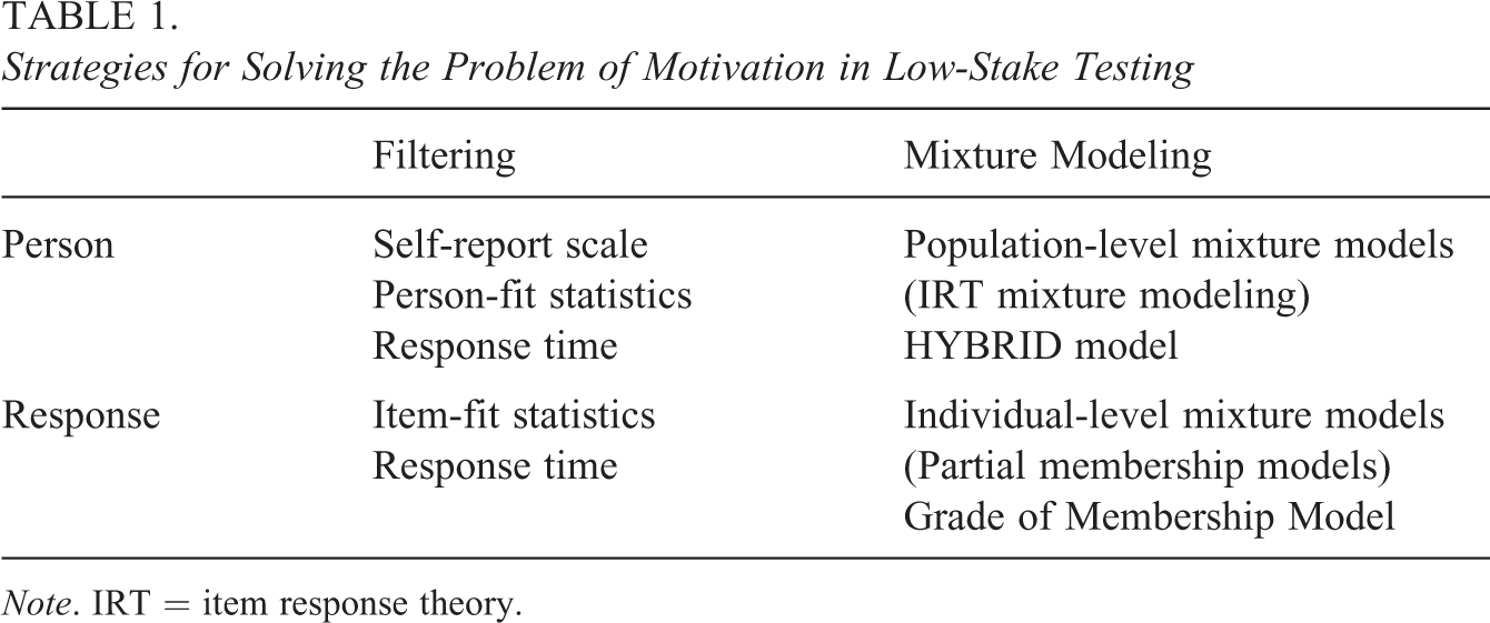
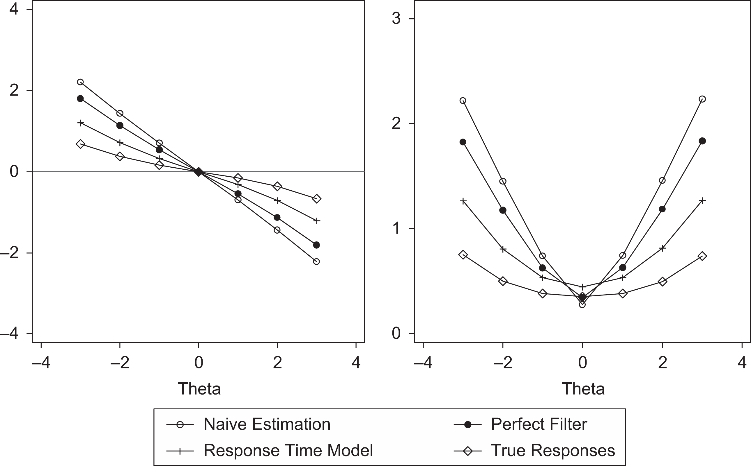
The Monte Carlo study was designed to validate the model by taking into account three factors: (1) separability of guessing and solution behaviors, (2) levels of guessing, and (3) correlation between guessing and latent trait. For the first factor, three conditions were specified: high, medium, and low. High separability was defined when the means of guessing and solution behavior times differed by 3.0 standard deviations. For medium separability, the difference was defined by 2.0 standard deviations. Low separability was defined by 1.0 standard deviation (see Figure 1). In the high-separability condition, the distribution of RT and guessing time barely overlapped. In the low-separability condition, two distributions almost fully overlapped. The high-separability condition represented a perfect situation when the distinction between solution and guessing behavior was easily made, and it was robust in a graphical examination. Although this situation is not likely to happen in real situations, it is a good starting point because even simple solutions, such as item filtering, should work well when virtually all guessing behaviors are identified. RTM is expected to be advantageous in situations where the identification of guessing behaviors is not straightforward because it does not require one to take so many arbitrary decisions while establishing the cut-off thresholds. Moreover, in RTM, all responses are kept providing some pieces of information, while in filtering process, when response is filtered out, some pieces of information are irretrievably lost.

Figure 1.

Different types of solution and guessing time distributions used in simulation studies.

The second factor indicates the level of guessing. Two levels of guessing were employed: 20% and 40%. Both levels are high and are be expected to occur in very low-stakes testing with little involvement of the respondents. It is well known that biases or the precision of estimates will increase with higher levels of guessing and decrease with lower levels of guessing. Because the main goal of the simulation is to compare different approaches, high levels of guessing were chosen in order to facilitate the interpretation of the results.

Finally, a third factor was employed to test the assumptions that need to be made in order for effective item filtering, but it is not obviously true in all situations (see Wise & DeMars, 2005). Two settings were specified for this factor. In the first setting, data were generated with a zero correlation between the probability of guessing and the latent trait. In the second setting, the correlation of 0.3 between guessing and the latent trait was generated.

Twelve settings were tested (3 × 2 × 2) and examined by using four approaches. In the first approach, the Rasch model was tested on observed data, ignoring the problem of guessing. As discussed in Section 4, this modeling is referred to as a naive approach. In the second approach, filtering using optimal threshold selection was used. As data were generated according to the known true model, the values of the thresholds that provided the highest rates identifying guessed responses and the lowest possible level of incorrect response classification according to the generating model were used. In Figure 1, these thresholds are identified by the intersection of the time density functions of the guessing and solution behavior. In this study, this approach is referred to as perfect filtering. The third approach uses the RMT as described by Equations 3, 4, and 7. Finally, the Rasch model is applied using true responses (i.e., in situation where guessing does not affect the data). This model was estimated as a reference model, the results of which were obtained without guessing behaviors.

The detailed description of data generation for the simulations is expressed in the following six points:

A total of 2,000 person-ability parameters (θs) for individuals were randomly drawn from a standard normal distribution.

Responses to 30 items for each individual were generated according to the Rasch model (item difficulties were sampled from a standard normal distribution). These responses are referred to as true responses.

For each true response, an indicator was generated indicating assignment to the solution class or to the guessing class (20% or 40% of guessing, depending on scenario). Assignment was generated either randomly or probability of guessing was related with ability. In the second scenario, 30 indicators of guessing were generated using 2PL model (similar to Step 2). For generating indicators of guessing, person-ability parameters from Step 1 were used. Difficulty and discrimination parameters were selected, such that the observed correlation between indicators of guessing and abilities equaled 0.3 (keeping assumed 20% or 40% of guessing).

If a true response was assigned to guessing class, new observed response uncorrelated with ability with probability of correct answer set to 0.2 was generated. If a true response was assigned to the solution class, it stayed the same for observed response. Therefore, observed responses reflect data that in real life are given to a researcher and are affected by guessing while true responses depict counterfactual situation showing what would happen if guessing does not exist.

Each response time or guessing time was sampled from different distributions of response time or guessing time.

The data estimation was conducted using Mplus 7.2 software in a generalized linear mixed modeling framework.

The procedure was repeated 400 times for each setting. No converged rate for each model was less than 10%. If one or more models did not converge for a particular replication, data set and all results were excluded from analysis and new replacement data generated.

4. Simulation Results

Bias and root mean square error (RMSE) were used to assess the accuracy of the parameter estimates in the 400 replications of the simulated settings. Bias is the average difference between an estimate and the true parameter value over the replications:

Bias (\hat{θ}) = \frac{1}{R} \sum_{r = 1}^{400} ({\hat{θ}}_{r} - θ),

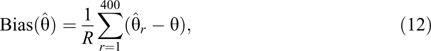
where ${\hat{θ}}_{r}$ is the estimated parameter for the rth replication, and θ is the true value of the parameters. RMSE indicates the overall accuracy of the parameter estimates:

RMSE (\hat{θ}) = \sqrt{\frac{1}{R} \sum_{r = 1}^{400} {({\hat{θ}}_{r} - θ)}^{2}} .

Both measures were reported by averaging each value over all items or ability parameter estimates in the data sets.

4.1 Item Parameter Estimates

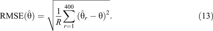
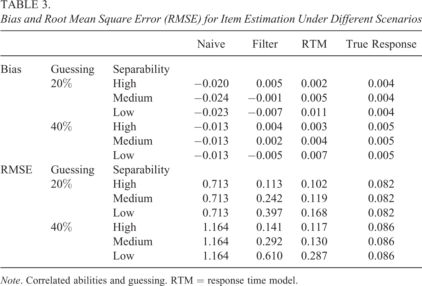
Table 2 presents results of the bias and RMSE for item difficulty under settings with no correlations between abilities and guessing. Each presented model is characterized by a very small overall bias. The reason that the average biases were so small is shown in Figure 2. These will be discussed later. The difference in estimation accuracy is shown in the RMSE results. All tested models behaved similar; the lower was separability, the higher was RMSE, and the higher was the proportion of guessing in the responses, RMSE was higher. Overall, RTM provided the smallest values of RMSE in all the settings presented in Table 2 (excluding the estimation on true responses). Perfect filtering provided accuracy similar to that given by RTM but only when separability was high. In medium and low separability, the RTM showed significantly greater accuracy than other tested models. The results of the naive approach confirmed the expectation that guessing behaviors would be a serious threat to the accuracy of the item parameters.

Table 2.

Bias and Root Mean Square Error (RMSE) for Item Estimation in Different Scenarios

			Naive	Filter	RTM	True Responses
Bias	Guessing	Separability
	20%	High	0.028	−0.004	−0.009	−0.006
		Medium	0.028	0.005	−0.010	−0.006
		Low	0.028	0.014	−0.016	−0.006
	40%	High	−0.068	−0.007	−0.001	−0.002
		Medium	−0.068	−0.017	0.001	−0.002
		Low	−0.068	−0.035	0.008	−0.002
RMSE	Guessing	Separability
	20%	High	0.751	0.109	0.099	0.084
		Medium	0.751	0.248	0.115	0.084
		Low	0.751	0.414	0.172	0.084
	40%	High	1.196	0.133	0.114	0.083
		Medium	1.196	0.298	0.131	0.083
		Low	1.196	0.643	0.405	0.083

Note. No correlation between abilities and guessing. RTM = response time model.

Figure 2.

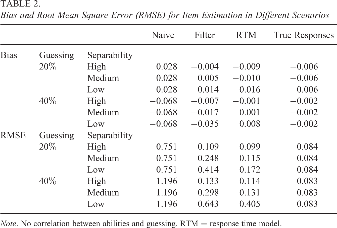
Relation between true item parameters and estimates using different methods. Low separability and 40% guessing. Correlated abilities and guessing.

Table 3 confirms the results obtained in settings where the correlation between latent traits was set to zero (Table 2). The results of the simulations in settings where relationships between guessing and proficiency estimates existed were similar to those shown in Table 2.

Table 3.

Bias and Root Mean Square Error (RMSE) for Item Estimation Under Different Scenarios

			Naive	Filter	RTM	True Response
Bias	Guessing	Separability
	20%	High	−0.020	0.005	0.002	0.004
		Medium	−0.024	−0.001	0.005	0.004
		Low	−0.023	−0.007	0.011	0.004
	40%	High	−0.013	0.004	0.003	0.005
		Medium	−0.013	0.002	0.004	0.005
		Low	−0.013	−0.005	0.007	0.005
RMSE	Guessing	Separability
	20%	High	0.713	0.113	0.102	0.082
		Medium	0.713	0.242	0.119	0.082
		Low	0.713	0.397	0.168	0.082
	40%	High	1.164	0.141	0.117	0.086
		Medium	1.164	0.292	0.130	0.086
		Low	1.164	0.610	0.287	0.086

Note. Correlated abilities and guessing. RTM = response time model.

Figure 2 shows the combined results of 400 simulations (30 items each) in the low-separability setting; 40% of the guessed responses and the correlation between ability and guessing was specified. The results of four types of estimation methods are scattered against the true parameters of items used in the data generating process. Figure 2 clearly explains the low values of the average bias reported for all models. The bias was symmetric and showed different signs on different sites of the item distribution for both the naive approach and item filtering. The item parameters shrank toward zero in both approaches. The great advantage of RTM over the naive and filtering approaches was that it provided results without any systematic bias in the distribution of all the item difficulties. This entailed a higher variation in item parameter estimation compared to estimation using true responses. However, it should be noted that the variation was not substantially higher than in the naive and filtering approaches.

4.2 Ability Estimates

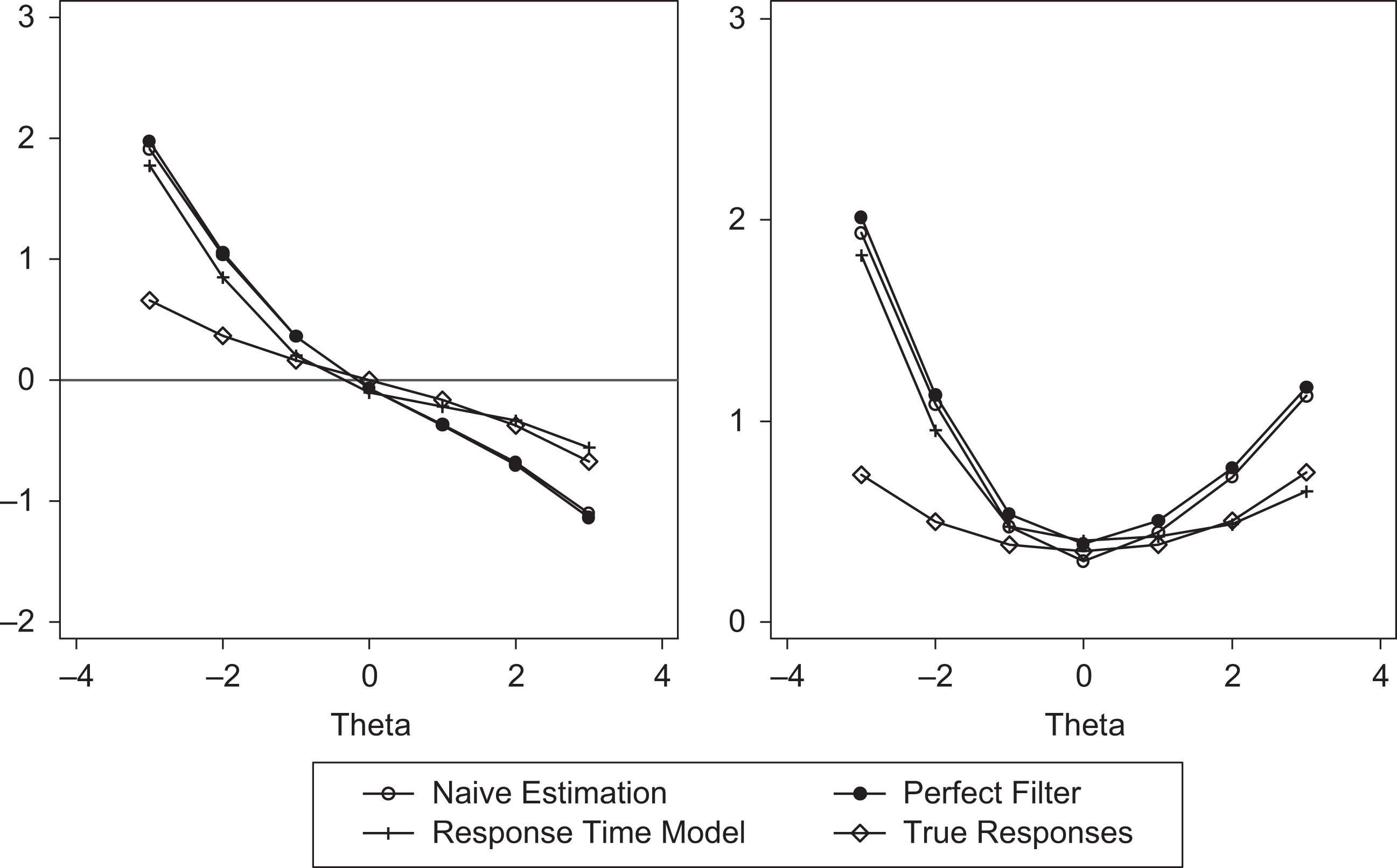
According to RMSE, the RTM performed the best in all settings. Figure 3 shows the bias and RMSE computed conditionally on ability distribution. The graph in Figure 3 shows the symmetrical nature of the bias and RMSE, which increased in high and low abilities. RTM also performed the best in this comparison.

Figure 3.

Bias and Root Mean Square Error (RMSE) for ability estimation under low separability and 40% guessing. No correlation between abilities and guessing.

In Table 4, the bias and RMSE for the ability parameters are presented in six scenarios. No correlation between abilities and guessing was specified. Similar to the results showing the average bias for items, bias for ability estimates is near zero. The RMSE measures showed differences between the selected estimation methods. According to RMSE, the RTM performed the best in all settings. Figure 3 shows the bias and RMSE computed conditionally for the ability distribution. This graph shows the symmetrical nature of the bias and RMSE, which increased for both high and low abilities. RTM also performed the best in this comparison.

Table 4.

Bias and Root Mean Square Error (RMSE) for Ability Estimation Under Different Scenarios

			Naive	Filter	RTM	True Response
Bias	Guessing	Separability
	20%	High	0.001	0.000	−0.001	0.000
		Medium	0.001	0.000	0.000	0.000
		Low	0.001	0.001	0.000	0.000
	40%	High	0.001	0.001	0.000	0.000
		Medium	0.001	0.001	0.001	0.000
		Low	0.001	0.002	0.001	0.000
RMS	Guessing	Separability
	20%	High	0.568	0.436	0.433	0.392
		Medium	0.568	0.464	0.445	0.392
		Low	0.568	0.500	0.457	0.392
	40%	High	0.715	0.489	0.485	0.392
		Medium	0.715	0.525	0.503	0.392
		Low	0.715	0.624	0.546	0.392

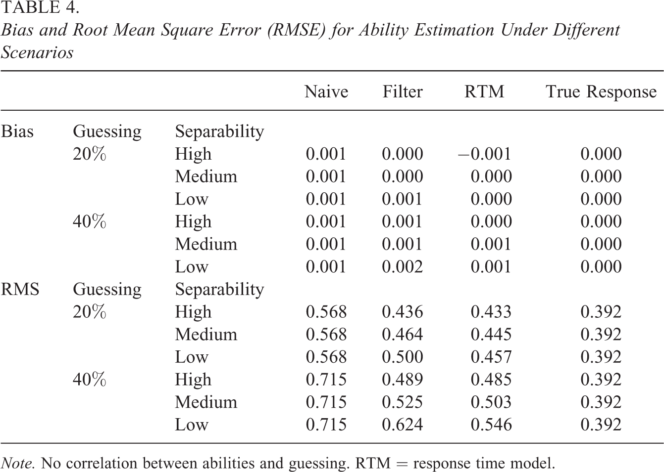
Note. No correlation between abilities and guessing. RTM = response time model.

Table 5 presents the bias and RMSE for the ability parameters in six scenarios where the correlation between abilities and guessing was specified. Similar to the previous results, the biases found in all methods approached zero. Only RMSE was differentiated in the investigated methods.

Table 5.

Bias and Root Mean Square Error (RMSE) for Ability Estimation Under Different Scenarios

			Naive	Filter	RTM	True Response
Bias	Guessing	Separability
	20%	High	−0.011	−0.015	−0.014	0.000
		Medium	−0.011	−0.013	−0.013	0.000
		Low	−0.011	−0.012	−0.011	0.000
	40%	High	−0.020	−0.024	−0.022	0.000
		Medium	−0.020	−0.022	−0.021	0.000
		Low	−0.020	−0.020	−0.017	0.000
RMSE	Guessing	Separability
	20%	High	0.409	0.447	0.448	0.393
		Medium	0.409	0.445	0.438	0.393
		Low	0.409	0.441	0.428	0.393
	40%	High	0.474	0.518	0.517	0.393
		Medium	0.474	0.519	0.508	0.393
		Low	0.474	0.538	0.475	0.393

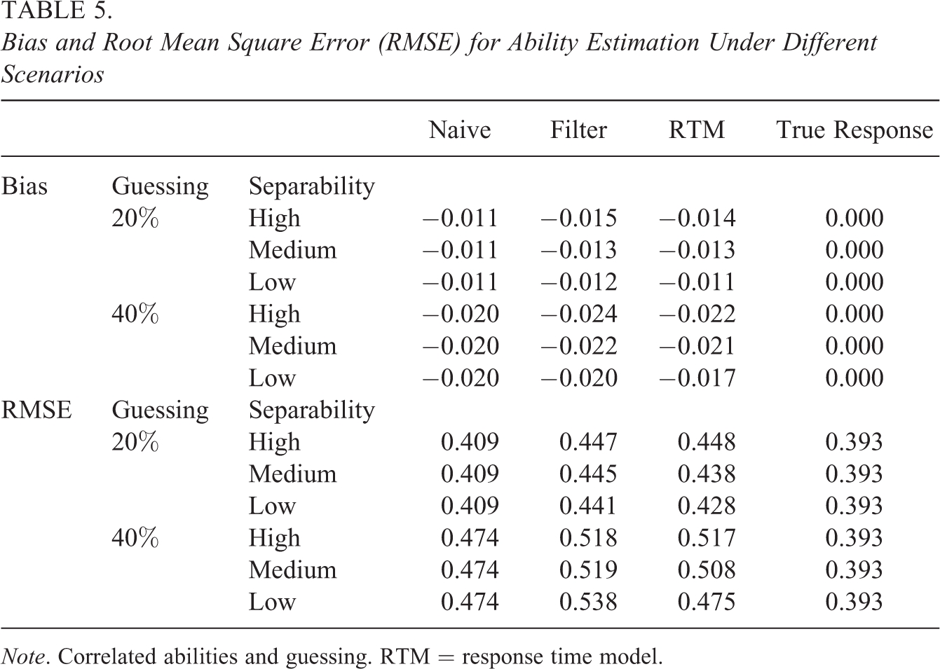
Note. Correlated abilities and guessing. RTM = response time model.

Figure 4 also shows bias and RMSE, which are plotted against levels of latent traits when the proportion of guessing equaled 40%, and latent trait was correlated with the guessing process. Because the correlation was negative in this setting (lower thetas have a higher probability of guessing), bias and RMSE were not perfect symmetrical. The person’s parameters for respondents with lower ability were estimated with lower precision. This happened because less information about ability estimation was provided for low-performing persons. Moreover, when ability is low, guessing looks very similar to actually trying, and RTM has low power to distinguish between two classes. It is noteworthy that all estimation methods produced high RMSE and high biases in the lower half of the θ distribution. In the upper half of the θ distribution, the naive approach and perfect filtering provided similar highly biased results with low accuracy. However, in this part of the distribution, RTM gave estimates similar to those obtained using true responses. These results are shown in Figure 5.

Figure 4.

Bias and Root Mean Square Error (RMSE) for ability estimation under low separability and 40% guessing. Correlated abilities and guessing.

Figure 5.

Relation between true item parameters and estimates using different methods. Low separability and 40% guessing. Correlated abilities and guessing.

In Figure 5, the scatterplots of the parameters of personal ability are plotted against the true level of latent traits in settings where the correlation between ability and guessing was set to 0.3, and the proportion of guessing was set to 0.4. All estimates in the lower part of the distribution were highly biased in all methods. In the upper part of the distribution, only RTM provided results similar to the true, not affected by guessing, data.

4.3 Detection of Guessing

In this section, results showing ability of RTM to identify a guessed versus motivated answer on individual responses are presented. Table 6 presents estimated proportion of guessing averaged over 400 replications (estimated guessing). Additionally, two indicators of errors in detecting guessing responses are presented: estimated percentage of solution strategies while true response was guessed (guessing wrongly classified) and estimated proportion of guessing behaviors among solution strategies (solution behaviors wrongly classified), both of those indicators were averaged over all replications. Results are presented for all simulation conditions.

Table 6.

Detection of Guessing Under Different Simulation Settings

Separability	Estimated Guessing	Guessing Wrongly Classified	Solution Behaviors Wrongly Classified	Estimated Guessing	Guessing Wrongly Classified	Solution Behaviors Wrongly Classified
	20% of guessing
	Abilities and guessing—Not correlated			Abilities and guessing—Correlated
High	20.30%	6.8%	2.10%	20.00%	8.9%	2.20%
Medium	21.70%	21.4%	7.50%	21.40%	23.3%	7.50%
Low	23.50%	33.7%	12.80%	23.00%	36.4%	12.80%
	40% of guessing
	Abilities and guessing—Not correlated			Abilities and guessing—Correlated
High	40.30%	3.6%	2.90%	39.60%	4.8%	2.90%
Medium	41.70%	11.7%	10.70%	40.90%	12.6%	10.10%
Low	46.70%	26.9%	29.20%	45.90%	27.7%	28.40%

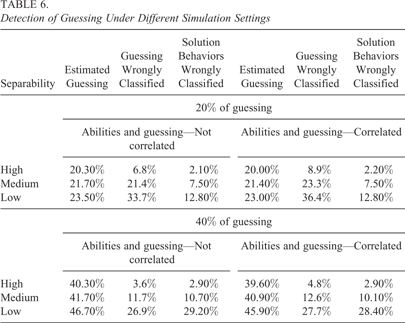
Overall results presented in Table 6 show that RTM provides a reasonably good tool for detecting guessing behaviors. With high separability (when response time is strongly related with guessing), estimated proportion of guessing and true proportion of guessing were virtually the same (with error smaller than 0.4%), both in the situation when abilities and guessing were correlated and when they were not. The proportions of wrongly classified responses were also small and independent of correlation between guessing and abilities. The model clearly loses its accuracy when separability becomes smaller. For medium separability, estimated proportion of guessing did not differ more than 1.7% from true proportion of guessing, while for low separability, overestimation of 6.7% was observed in condition with 40% of true guessing (in setting with no correlation between guessing and abilities).

The results presented in Table 6 are suggesting important advantage and practical usefulness of the RTM. Even if unbiased recovery of abilities is not possible in some scenarios (see Section 4.2), RTM could successfully detect at least the overall proportion of guessing. Of course, the better the predictors of guessing are, the more accurate result would be obtained.

5. Empirical Data: Example

The PIAAC was chosen to illustrate the application of the RTM. In PIAAC, approximately 166,000 adults aged 16 to 65 years were surveyed in the subregions of 24 countries/national. PIAAC has two main components: a background questionnaire and an assessment of literacy, numeracy, and problem-solving in a technology-rich environment. The questionnaire was administered first and then the respondents completed a cognitive assessment that took approximately 1 hr to complete. Depending on the respondents’ computer skills, the assessments were delivered on either a laptop computer or as a fill-in paper booklet (see Organization for Economic Co-operation and Development [OECD], 2013, and www.oecd.org/site/piaac for technical details).

For this study a numeracy scale was reestimated in all PIAAC countries, except Russia because of inconsistencies in the Russian data (see OECD, 2013). The original PIAAC scale was estimated by 2PL model that used both paper-and-pencil assessment and CBA, concurrently. Because RTM requires timing information that is available only in CBA, the respondents who completed paper booklets were excluded from this analysis. This exclusion reduced the initial sample size by 50%. Considerable variation in the percentage of CBA test takers among countries was present (for details, see OECD, 2013). On average, CBA test takers performed better; therefore, reduced sample is not directly comparable with initial PIAAC sample. Additionally, as some response times in the data were found to be implausible, very long response times (higher than 3 standard deviations above mean) were recorded as missing.

The original PIAAC results are presented on a scale where the country mean is around 250 and the standard deviation is around 50 (see www.oecd.org/site/piaac). The rescaled results using the Rasch model are presented in a logistic metric where the mean of the country with the lowest results was set at 0.

The RTMs described by Equations 9 and 10 were estimated on the PIAAC numeracy items and compared with the simple Rasch and 2PL models. In total, four models—Rasch, 2PL, Rasch-RTM, and 2PL-RTM—were estimated. The time variable for each response was operationalized as the difference between the mean response time for a particular item and the actual response. The multigroup structure was reflected by using the Rasch and 2PL model to estimate the country-specific means. Table 7 shows that according to Akaike information criterion and Bayesian information criterion measures, simple models ignoring guessing fit data significantly worse than RTMs (2PL model fits slightly better than Rasch). Among RTMs, 2PL-RTM showed considerably better fit than Rasch-RTM.

Table 7.

Measures of Fit for the Rasch Model and RTM Estimated Using the PIAAC Numeracy Items

	AIC	BIC
Rasch	1,887,491.587	1,888,429.206
2PL	1,876,084.337	1,877,659.538
Rasch-RTM	1,691,814.038	1,692,746.028
2PL-RTM	1,569,686.504	1,571,249.344

Note. AIC = Akaike information criterion; BIC = Bayesian information criterion; 2PL = two-parameter logistic; RTM = response time model; PIAAC = Programme for the International Assessment of Adult Competencies.

Table 8 shows the results of the original scale and estimated four models. It also shows the proportion of guessing responses estimated by the RTMs. As 2PL-RTM fits best to the data, the description of the results focuses on this model. The results clearly revealed some variability in the estimated proportions of the guessed items from country to country. The average proportion was 9.36% (higher than for Rasch-RTM which was 7.4%). Italy, Sweden, France, Cyprus, and Flanders showed the largest estimates of guessing behaviors (more than 10%) of responses while Korea, Japan, and Poland showed the lowest proportion at smaller than 5%. However, adjusting the scale for guessing did not change the country ranking dramatically between 2PL and 2PL-RTM estimation (the country-level correlation between two scales equals 0.995). The main difference was that the RTM results showed higher variation between countries. These results are supported by the simulated results that showed a higher bias in the naive approach on the edges of the distributions. RTM-2PL therefore provides better picture of cross-country differences in average results.

Table 8.

Country Means in PIAAC Numeracy Scale Using Different Approaches

	PIAAC	Rasch	2PL	Rasch-RTM		2PL-RTM
Country	Mean	Mean	Mean	Guessing (%)	Mean	Guessing (%)	Mean
Japan	288	1.272	1.090	11.5	1.327	4.1	1.240
Finland	282	0.973	0.761	5.2	0.991	7.9	0.945
Flanders (Belgium)	280	0.713	0.546	13.8	0.696	12.9	0.656
The Netherlands	280	0.793	0.580	8.4	0.816	9.4	0.710
Sweden	279	0.820	0.649	8.5	0.837	14.3	0.786
Norway	278	0.767	0.617	7.5	0.755	7.8	0.714
Denmark	278	0.798	0.621	7.9	0.805	9.0	0.739
Slovak Republic	276	0.769	0.629	5.3	0.769	9.8	0.665
Czech Republic	276	0.704	0.525	5.0	0.703	10.9	0.621
Austria	275	0.771	0.571	11.1	0.756	9.7	0.682
Estonia	273	0.664	0.540	6.2	0.671	7.7	0.598
Germany	272	0.682	0.506	5.9	0.659	7.2	0.604
Australia	268	0.557	0.456	6.9	0.574	7.4	0.536
Canada	265	0.400	0.289	7.0	0.412	9.7	0.341
Cyprus	265	0.319	0.244	6.3	0.367	13.2	0.236
Korea	263	0.476	0.471	4.7	0.421	3.7	0.548
England/Northern Ireland (UK)	262	0.317	0.246	7.0	0.314	9.4	0.309
Poland	260	0.414	0.366	4.0	0.409	4.7	0.397
Ireland	256	0.261	0.203	7.0	0.281	10.4	0.213
France	254	0.198	0.125	8.4	0.273	13.9	0.143
United States	253	0.083	0.089	7.1	0.013	7.6	0.124
Italy	247	0.033	0.035	9.7	0.137	15.1	−0.003
Spain	246	0.000	0.000	5.9	0.000	9.5	0.000

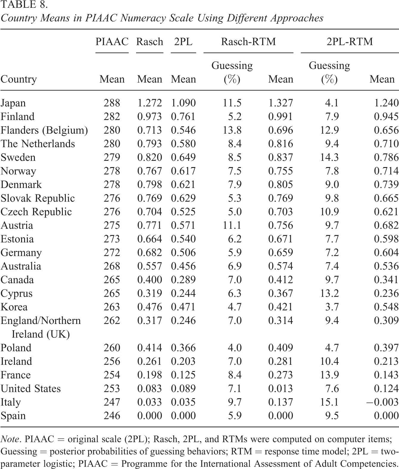
Note. PIAAC = original scale (2PL); Rasch, 2PL, and RTMs were computed on computer items; Guessing = posterior probabilities of guessing behaviors; RTM = response time model; 2PL = two-parameter logistic; PIAAC = Programme for the International Assessment of Adult Competencies.

Small changes in country position indicated that random guessing was not strongly related to ability. In fact, the correlation between estimated ability and probability of guessing in the PIAAC data on respondent level was very small at −0.13; thus, it did not substantially alter the results for the countries.

Overall, the RTMs fit to the real data better than other models that ignore guessing. Country rankings remain very similar, but this does not indicate that the presented models are not more accurate. If we compare Rasch model with 2PL model, also the differences in the country rankings are not very large but it does not mean that 2PL model brings no improvement over Rasch model. RTMs introduced important correction to model that ignores guessing showing higher between countries variation in means and minor corrections in rankings.

6. Summary and Discussion

This article reported a study that tested a new method based on the GoM model. The RTM has substantial promise as a method for managing the problems of guessing behaviors in low-stake test situations. The results demonstrated that ignoring the problem of guessing seriously biased the results and that the new RTM outperformed the existing methods in all simulated conditions.

RTM seems to be well suited to many situations involving low-stake tests, including large-scale assessments, such as PISA, PIAAC, or Progress in International Reading Literacy Study (PIRLS), where motivation might influence the results of particular students and particular groups. Using RTM on PIAAC data did not drastically change the results. Instead, it provided a small correction, which led to an even more precise estimation of group differences. However, it is not guaranteed that for different data, such as on younger respondents in PISA or PIRLS, the corrections also would be so small. This is an empirical question. If RTM is not used as the ultimate model for producing final results, it should be at least used to test the robustness of other models and assumptions about guessing.

Large-scale assessments are not the only area in which RTM may prove to be a valuable solution. Item banking, equating, and linking studies in which some parts of research are conducted under lower motivation conditions might lead to more precise and unbiased estimates of item parameters and ability distributions. RTM could be used not only in testing context but also in personality scales, attitude surveys, and all measurement situations where motivation is suspected to be low. Using appropriate data, this model could also be used to deepen the understanding of the process of guessing. With proper item-level and respondent-level covariates, future research could investigate the interactions between factors that trigger guessing behaviors. This knowledge could be used to design measurement instruments that minimalize the provocation of guessing.

The greatest advantage of the RTM is that it might be estimated using existing software and ML estimation. Appendices A and B present the syntax for the Mplus computer program showing the RTMs used in this study. The disadvantage of the proposed solution is that even with fast modern computers, the estimation of the model is very slow. It took 48 hr to estimate the results for Rasch model presented in Table 8, days for 2PL-RTM, and almost 6 months to conduct the Monte Carlo study. Optimizing the estimation of the model involves serious work. The most problematic assumption of the presented models is that latent traits are independent of covariates conditional on the LC, that is, response time is not correlated with abilities after controlling for the categorical latent variables, defining solution, and guessing class. In some situations, this assumption could be considered implausible. Fortunately, the RTM could be easily expanded to abolish this assumption by redefining the response model in the solution behaviors class. The latent linear logistic test model (LLTM) could be easily used to incorporate the time variable into the response function. Alternatively, the latent regression LLTM (De Boeck & Wilson, 2004) could be specified when a greater number of LC predictors were correlated with ability on both individual and item levels. Future research should perform further simulations to prove whether such steps would reduce potential biases.

It is also worth it to emphasize that guessing behavior is a complicated phenomenon of interaction between person, item, and testing occasion characteristics. Guessing can be a rational strategy of a motivated respondent who is not able to solve the problem, consequently being a solution response behavior. Guessing may result from lack of motivation to make an effort to solve the problem, which would otherwise be within reach of the respondents’ skills. In this article, only the latter case was considered as “guessing behavior.” This type of guessing was connected with the assumption that longer response time implies less guessing, that is, less-motivated respondents are going fast through the items to the end of the test.

Footnotes

Appendix A

Appendix B

Declaration of Conflicting Interests

The author(s) declared the following potential conflicts of interest with respect to the research, authorship, and/or publication of this article.

Funding

The author(s) disclosed receipt of the following financial support for the research, authorship, and/or publication of this article: This work has been prepared under the Project From School to Work: Individual and Institutional Determinants of Educational and Occupational Career Trajectories of Young Poles, which is funded by the Polish National Science Centre, as part of the grant competition Maestro 3 (UMO-2012/06/A/HS6/00323).

References

Airoldi

E. M.

Blei

D. M.

Erosheva

E. A.

Fienberg

S. E.

(2014). Introduction to mixed membership models and methods. In Airoldi

E. M.

Blei

Erosheva

E. A.

Fienberg

S. E.

(Eds.), Handbook of mixed membership models and their applications (pp. 3–14). Boca Raton, FL: Chapman & Hall/CRC.

Asparouhov

Muthén

(2008). Multilevel mixture models. In Hancock

G. R.

Samuelsen

K. M.

(Eds.), Advances in latent variable mixture models (pp. 27–51). Charlotte, NC: IAP.

Dayton

C. M.

Macready

G. B.

(1988). Concomitant-variable latent-class models. Journal of the American Statistical Association, 83, 173–178.

De Boeck

Wilson

(2004). A framework for item response models (pp. 3–41). New York, NY: Springer.

Dempster

A. P.

Laird

N. M.

Rubin

D. B.

(1977). Maximum likelihood from incomplete data via the EM algorithm. Journal of the Royal Statistical Society. Series B (methodological), 39, 1–38.

Erosheva

E. A.

(2002). Grade of membership and latent structure models with application to disability survey data (Doctoral dissertation). Office of Population Research, Princeton University, Princeton, NJ.

Erosheva

E. A.

(2005). Comparing latent structures of the Grade of Membership, Rasch, and latent class models. Psychometrika, 70, 619–628.

Gruhl

Erosheva

E. A.

(2013). A tale of two (types of) memberships: Comparing mixed and partial membership with a continuous data example. In Airoldi

E. M.

Blei

Erosheva

E. A.

Fienberg

S. E.

(Eds.), Handbook of mixed membership models and their applications (pp. 15–38). Chapman & Hall/CRC.

Mislevy

R. J.

Verhelst

(1990). Modeling item responses when different subjects employ different solution strategies. Psychometrika, 55, 195–215.

10.

Muthén

L. K.

Muthén

B. O.

(1998–2015). Mplus User's Guide. Seventh Edition. Los Angeles, CA: Muthén & Muthén.

11.

Organization for Economic Co-operation and Development. (2013). OECD skills outlook 2013: first results from the survey of adult skills. Paris: Author. Retrieved from http://dx.doi.org/10.1787/9789264204256-en

12.

O’Neil

H. F.

Sugrue

Baker

E. L.

Jr (1995). Effects of motivational interventions on the National Assessment of Educational Progress mathematics performance. Educational Assessment, 3, 135–157.

13.

Rost

(1991). A logistic mixture distribution model for polychotomous item responses. British Journal of Mathematical and Statistical Psychology, 44, 75–92.

14.

Schnipke

D. L.

Scrams

D. J.

(1997). Modeling item response times with a two-state mixture model: A new method of measuring speededness. Journal of Educational Measurement, 34, 213–232.

15.

Smit

Kelderman

van der Flier

(1999). Collateral information and mixed Rasch models. Methods of Psychological Research Online, 4, 19–32.

16.

Smit

Kelderman

van der Flier

(2000). The mixed Birnbaum model: Estimation using collateral information. Methods of Psychological Research Online, 5, 31–43.

17.

Sundre

D. L.

Kitsantas

(2004). An exploration of the psychology of the examinee: Can examinee self-regulation and test-taking motivation predict consequential and non-consequential test performance? Contemporary Educational Psychology, 29, 6–26.

18.

Thelk

A. D.

Sundre

D. L.

Horst

S. J.

Finney

S. J.

(2009). Motivation matters: Using the Student Opinion Scale to make valid inferences about student performance. The Journal of General Education, 58, 129–151.

19.

Vermunt

J. K.

Magidson

(2005). Factor analysis with categorical indicators: A comparison between traditional and latent class approaches. In Van der Ark

Croon

M. A.

Sijtsma

(Eds.), New developments in categorical data analysis for the social and behavioral sciences (pp. 41–62). Mahwah, NJ: Lawrence Erlbaum.

20.

von Davier

Yamamoto

(2007). Mixture-distribution and HYBRID Rasch models. In von Davier

Carstensen

C. H.

(Eds.), Multivariate and mixture distribution Rasch models (pp. 99–115). New York, NY: Springer.

21.

Wise

S. L.

DeMars

C. E.

(2005). Low examinee effort in low-stakes assessment: Problems and potential solutions. Educational Assessment, 10, 1–17.

22.

Wise

S. L.

Kong

(2005). Response time effort: A new measure of examinee motivation in computer-based tests. Applied Measurement in Education, 18, 163–183.

23.

Wise

S. L.

Bhola

D. S.

Yang

S. T.

(2006). Taking the time to improve the validity of low-stakes tests: The effort-monitoring CBT. Educational Measurement: Issues and Practice, 25, 21–30.

24.

Wise

S. L.

Kingsbury

G. G.

Hauser

(2010, 5). An investigation of the relationship between time of testing and test-taking effort. Paper presented at the annual meeting of the National Council on Measurement in Education, Denver, CO.

25.

Wolf

L. F.

Smith

J. K.

Birnbaum

M. E.

(1995). Consequence of performance, test, motivation, and mentally taxing items. Applied Measurement in Education, 8, 341–351.

26.

Yamamoto

(1989). A Hybrid model of IRT and latent class models. ETS Research Report Series. Princeton, New Jersey: Educational Testing Service.

27.

Yamamoto

Everson

(1997). Modeling the effects of test length and test time on parameter estimation using the HYBRID model. In Rost

Langeheine

(Eds.), Applications of latent trait and latent class models in the social sciences (pp. 89–98). New York, NY: Waxmann Verlag GmbH.