Estimation of Indirect Effects in the Presence of Unmeasured Confounding for the Mediator–Outcome Relationship in a Multilevel 2-1-1 Mediation Model

Abstract

To assess the direct and indirect effect of an intervention, multilevel 2-1-1 studies with intervention randomized at the upper (class) level and mediator and outcome measured at the lower (student) level are frequently used in educational research. In such studies, the mediation process may flow through the student-level mediator (the within indirect effect) or a class-aggregated mediator (the contextual indirect effect). In this article, we cast mediation analysis within the counterfactual framework and clarify the assumptions that are needed to identify the within and contextual indirect effect. We show that unlike the contextual indirect effect, the within indirect effect can be unbiasedly estimated in linear models in the presence of unmeasured confounders of the mediator–outcome relationship at the upper level that exert additive effects on mediator and outcome. When unmeasured confounding occurs at the individual level, both indirect effects are no longer identified. We propose sensitivity analyses to assess the robustness of the within and contextual indirect effect under lower and upper-level confounding, respectively.

Keywords

mediation multilevel 2-1-1 settings indirect effect counterfactual framework

To assess the impact of instructional methods on students’ performance, cluster-randomized trials have become the gold standard in educational psychology. Such designs are useful when entire classes are the focus of the intervention. They allow one, for instances, to estimate the causal relationship between teacher behavior and students’ engagement in learning and achievement. Unraveling this causal relationship may further deepen the understanding into the underlying processes. For example, Eccles’s expectancy-value model of achievement motivation (Wigfield & Eccles, 2000) links instructional style, motivational factors, and achievement, whereby performances are assumed to be influenced by students’ motivational beliefs, which themselves are influenced by students’ perceptions of teachers’ behavior. Mediation analysis allows one to test such theories and can disentangle the effect of a treatment or intervention T on an outcome Y into the effect going through a mediating variable M, called the mediator, and the remaining direct effect.

Multilevel models that account for the hierarchical nature of educational data are typically used to address mediation in cluster-randomized trials (MacKinnon, 2008). When the treatment is randomized at the upper (or second) level, but the mediator and outcome are measured at the lower (or first) level, this multilevel mediation setting is sometimes referred to as a 2-1-1 setting. There is currently much debate on how mediation may operate in this setting. Pituch and Stapleton (2012) nicely summarize the two prevailing opposing views. On the one hand, Preacher and colleagues (Preacher, Zyphur, & Zhang, 2010; Zhang, Zyphur, & Preacher, 2009) argue that “The effect of T on Y must be a strictly Between; because T is constant within a given group, variation in T cannot influence individual differences within a group” (Preacher et al., 2010, p. 210). In other words, they assert that a student-level variable cannot mediate the association between an intervention at the teacher level and an outcome measured at the student level and regard any association between the student-level mediator and outcome as irrelevant. These authors therefore purely focus on mediation processes at the cluster-level (left panel of Figure 1) or cluster-level only mediation. Other scholars (Krull & Mackinnon, 2001; Pituch & Stapleton, 2012; VanderWeele, 2010) argue that a teacher-level treatment may impact a student-level outcome through a student-level mediator. This is referred to as cross-level mediation. These authors allow that the effect of the intervention on the outcome may be mediated not only by a variable at the student level but also through a class-level aggregate of this mediator (right panel of Figure 1). We take the latter view and, in this article, particularly focus on the estimation of the indirect effect through the student-level mediator that will be referred to as the within indirect effect.

Figure 1.

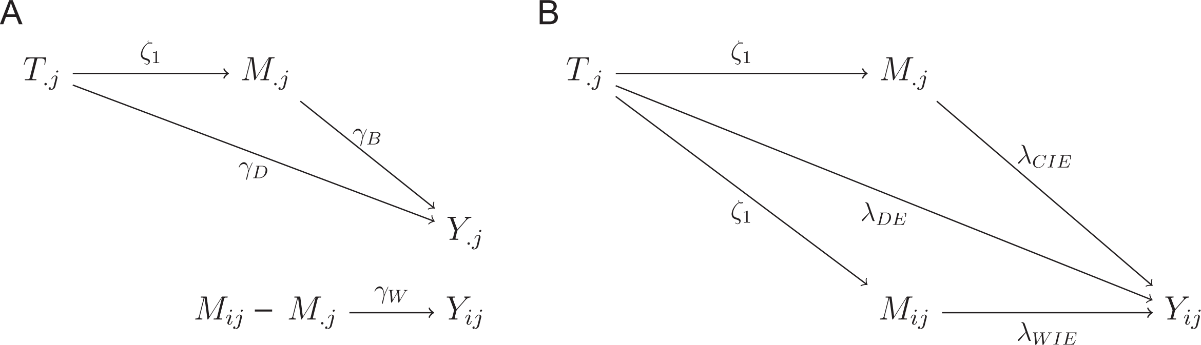
(A) The indirect effect in a 2-1-1 setting following the view of Zhang, Zyphur, and Preacher (2009). (B) The indirect effect in a 2-1-1 setting following the view of Pituch and Stapleton (2012).

The rationale for focusing on the within indirect effect can be understood from the illustrating example that we will use throughout this article. In a randomized experimental study, De Naeghel, Van Keer, Vansteenkiste, Haerens, and Aelterman (in press) evaluated the impact of a need-supportive teacher training grounded on self-determination theory. The experimental condition consisted of 12 teachers participating in a teacher professional development workshop (throughout this article referred to as “training”) aimed at providing the knowledge and skills necessary to implement an autonomy-supportive and structuring teaching style, whereas the control condition included 25 teachers who continued their current teaching repertoire. The researchers hypothesized that need-supportive teachers would change the autonomous reading motivation in fifth-grade students, which in turn would change reading frequency. Reading motivation was measured using the self regulation questionnaire (SRQ)-Reading Motivation (De Naeghel, Van Keer, Vansteenkiste, & Rosseel, 2012). To obtain a score for autonomous motivation, the average over the 17 items of this questionnaire, each measured on a 5-point Likert-type scale, was calculated. The reading frequency of students was measured as the average over 4 items on a 4-point Likert-type scale (1 = (almost) never, 2 = sometimes, 3 = often, 4 = (almost) always). For both measures, a pretest and posttest were obtained from 628 fifth-grade students from 37 classes in total. Note that it is an unbalanced design with an average group size of 17 (min = 7, max = 28). We consider for both autonomous reading motivation and reading frequency the change between scores on posttest and pretest. Since the researchers hypothesized that the effect of the need-supportive teaching style on individual reading performance change occurs via the individual autonomous motivation change of each student, we concur with Pituch and Stapleton (2012) that the cluster-level only mediation approach would not be well suited for this example. In the cross-level approach that we will consider, two mediated effects are of interest: the first through the individual change in autonomous motivation of the student and the second through the class-level aggregate of this mediator. This can be understood upon noting that the association between a student-level mediator and the outcome within a class, known as the within-group association, may be different from the association between the class means of the mediator and the outcome, known as the between-group association. This may be due to confounding factors; for example, classes may differ among each other in terms of factors such as socioeconomic status of the students, education level, and so on, which may be related to the outcome too. However, there may also be a difference because the between-group association measures a truly different effect. In many cases, there is thus no reason to assume that the within effects and between effects are similar; the contextual effect is formally defined as the difference between these two effects. While it is clear that in our motivating example, we are primarily interested in the effect of the teacher’s training on the student’s reading frequency through the change in the student’s reading motivation, interest in other settings may lie in the contextual indirect effect (e.g., Nagengast & Marsh, 2012).

In this article, we will clarify the assumptions under which the within and contextual indirect effects in the cross-level approach can be identified. We will therefore cast mediation analysis within the counterfactual framework. This framework has proved its usefulness in making the assumptions needed to identify direct and indirect effects in simple settings with independent observations more explicit. With a few notable exceptions (VanderWeele, 2010; VanderWeele, Hong, Jones, & Brown, 2013), such investigations are mostly absent in multilevel mediation settings as the one described here (Preacher, 2015). One particular complication in this context is interference, which is present when the treatment received by one individual may affect the outcomes of other individuals. This complication is not addressed by most of the literature on causal inference, which relies on an assumption of “no interference” (Tchetgen & VanderWeele, 2012). In particular, within Rubin’s (1976) causal framework, an assumption referred to as the “Stable Unit Treatment Value Assumption” includes a no-interference assumption. Under no interference, there is a single value of each potential outcome associated with each intervention for each student, regardless of how interventions are assigned and of which interventions are received by other students. Rubin (1980) cautioned that this assumption becomes problematic in educational settings, for example, where interventions are given to students who interact with each other in class. In our setting, when students in the same class experience higher autonomous motivation due to a need-supportive teacher, not only the individual change in autonomous motivation but also the changed autonomous motivation as a group may lead to a higher reading frequency in each student. Building on work by Hong and Raudenbush (2006) and VanderWeele, Hong, Jones, and Brown (2013), we present a potential outcome framework for causal inference in which not only one’s own but also the treatment of classmates can affect students’ potential outcome. This framework will enable us to obtain identification results for within and contextual indirect effects.

This article is further organized as follows: We first describe the multilevel approach proposed by Pituch and Stapleton (2012) aiming to estimate the within and contextual indirect effect and contrast it with an approach based on regression of differences (the ROD approach). The latter approach is also referred to as the “fixed effect” approach, the most common approach in the econometrics literature for handling upper-level confounding in panel data (Hausman & Taylor, 1981). Inspired by the work of Raudenbush and Willms (1995), the fixed effect approach has recently been introduced in the educational setting by Castellano, Rabe-Hesketh, and Skrondal (2014) for cross-sectional data. These authors show that this approach is preferable over more common approaches in educational research that estimate contextual effects by including class means of student covariates in addition to student-level covariates, particularly when there are unmeasured common causes of the predictor and outcome at the class level. In this article, we elaborate on their findings in the mediation setting and assess the impact of unmeasured confounding (i.e., unmeasured common causes) of the M-Y relationship at the upper and lower level on the estimation of within and contextual indirect effects. We show that in the presence of unmeasured upper-level M-Y confounders that exert an additive effect on mediator and outcome, the within indirect effect can still be unbiasedly estimated by both approaches in the linear models that we consider. We further derive bias expressions for the Pituch and Stapleton estimator of the contextual indirect effect in the presence of unmeasured upper-level M-Y confounding. In the presence of unmeasured lower-level M-Y confounding, the within indirect effect is no longer identified. We therefore propose a sensitivity analysis within the ROD framework that allows us to explore how the estimated within indirect effect is affected by violations of the no unmeasured lower-level M-Y confounding assumption. When interest lies in the contextual indirect effect, a sensitivity analysis in the Pituch and Stapleton framework can be performed to assess the impact of upper-level M-Y confounding. The ROD approach and the sensitivity analysis are illustrated with our motivating example. For ease of exposition, we focus primarily on simple settings with no interactions (i.e., no treatment mediator, treatment baseline covariate, or mediator baseline covariate interactions) but illustrate later how ideas extend to more complex settings involving such interactions. We end with a discussion.

Identification of the Direct and Indirect Effects in a 2-1-1 Model

The Counterfactual Framework

We first introduce some notation for the observed variables in a randomized 2-1-1 multilevel setting. Assume there is a random sample of K classes with sample sizes n ₁, n ₂, …, n_K . Let T_.j denote a binary treatment variable for group j (j = 1, … , K), which takes the value 1 for the experimental condition and 0 for the control condition. M_ij and Y_ij represent the mediator and outcome of student i (i = 1, … , n_j ) in group j, respectively. The vector C_ij collects all measured baseline covariates at individual and group level and contains information about cluster membership. For example, if measured, the number of years of teacher experience and the distance between the student’s home and the closest public library could be considered as covariate at, respectively, the group and individual level.

To define total, direct, and indirect effects in the 2-1-1 multilevel mediation setting, we will rely on the counterfactual framework of causal inference (Pearl, 2001; Robins & Greenland, 1992). A counterfactual or potential outcome Y_ij (t) is the outcome that would be observed in individual i (i = 1, … , n_j ) of cluster j (j = 1, … , K) if (possibly contrary to the fact) the group-level treatment T_.j in cluster j is set to t. Given a binary treatment, each individual has two potential outcomes, Y_ij (1) and Y_ij (0). In order to observe at least one of the potential outcomes for each subject, we need to make the consistency assumption for the outcome, which implies that the potential outcome for a given treatment T = t equals the observed outcome for subjects that are exposed to treatment t (VanderWeele, 2008). This assumption holds by design in randomized studies but may be more questionable with less manipulable treatments that are often seen in observational studies. While the individual total causal effect, defined as Y_ij (1) − Y_ij (0), cannot be calculated since individuals are only observed under a single intervention, the average total causal effect of treatment E(Y_ij (1) − Y_ij (0)) is identified as E(Y_ij|T_.j=1)−E(Y_ij|T_.j=0) in randomized trials; this latter difference can easily be estimated based on the observed data. We further make the intact cluster assumption (Hong & Raudenbush, 2008), which implies that the cluster to which individuals belong does not change because of the interventions at the cluster level. In educational research, this assumption generally holds since the intervention does not lead to reorganization of class groups. Note that for observational studies, one would additionally need to assume that there are no unmeasured confounders for the treatment–outcome relation. Similarly, let M_ij (1) and M_ij (0) represent the counterfactuals for the mediator under experimental and control condition, which can be used to define the causal effect on the mediator. In a randomized trial, the latter is identified as E(M_ij|T_.j=1)−E(M_ij|T_.j=0) when making the consistency assumption for the mediator and can be unbiasedly estimated based on the observed data.

To define direct and indirect effects, we need to introduce additional counterfactuals that are more complex than in the simple setting with independent observations. Spillover effects occur when the exposure of one individual affects the outcomes of other individuals. This phenomenon of spillover, also referred to as “interference,” is common whenever an outcome depends upon social interactions between individuals (VanderWeele, 2015). Similar to VanderWeele et al. (2013), we relax the no-interference assumption at the individual level by explicitly accounting for contextual effects through a function $f (M_{- i j}^{*})$ of all individual mediator values in cluster j excluding the mediator value of individual i. Although any function could be used, we will simply consider the average value of the mediator over all individuals in group j, other than i, which is denoted as M _−ij. In our illustrating example, M _−ij indicates the average change in autonomous reading motivation since the first measurement of all classmates of student i in class j. We introduce the nested counterfactual $Y_{i j} (t, M_{i j} (t^{'}), M_{- i j} (t^{*}))$ as the potential outcome that would have been observed in individual i of cluster j if treatment in cluster j was set to t and the student’s mediator M_ij and the mediators M _−ij of the classmates to the value that would have been observed under treatment t′ and t*, respectively. Further, let Y_ij (t, m, g) denote the counterfactual outcome for individual i in group j if T_.j (e.g., teacher training), M_ij (e.g., individual change in autonomous reading motivation), and M _−ij (e.g., average change in autonomous reading motivation) were set to, respectively, t, m, and g. While we do relax the no-interference assumption at the individual level, we still need to make the no interference between units—assumption at the group level implying that an individual’s mediator and outcome do not depend on the treatment assigned to clusters other than the individual’s own cluster (VanderWeele, 2010). This will for example be satisfied if each class belongs to a different school, and schools are sufficiently geographically separated.

With the definition of these nested counterfactuals, the average total causal effect can be decomposed into a natural direct effect (NDE) and a natural indirect effect (NIE):

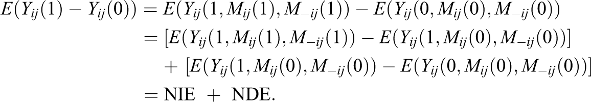
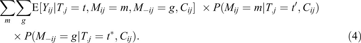
\begin{matrix} E (Y_{i j} (1) - Y_{i j} (0)) = E (Y_{i j} (1, M_{i j} (1), M_{- i j} (1)) - E (Y_{i j} (0, M_{i j} (0), M_{- i j} (0)) \\ = [E (Y_{i j} (1, M_{i j} (1), M_{- i j} (1)) - E (Y_{i j} (1, M_{i j} (0), M_{- i j} (0))] \\ + [E (Y_{i j} (1, M_{i j} (0), M_{- i j} (0)) - E (Y_{i j} (0, M_{i j} (0), M_{- i j} (0))] \\ = NIE + NDE. \end{matrix}

In our example, the NDE reflects the difference in reading frequency change for a need-supportive teacher versus a control teacher, while fixing the autonomous motivation of the student and the average autonomous motivation of his or her classmates to the level that would have been observed under the control condition. A simple way to view this is to note that values change for Y’s first arguments, but not for second and third, implying that Y is influenced by T only directly. The NIE reflects the difference in reading frequency change when the autonomous motivation of the student and the average autonomous motivation of his or her classmates changes from the level that would have been observed with a need-supportive trained teacher to the level that would have been observed in the control group, while fixing the intervention to the experimental condition otherwise. Now the first argument of Y is fixed, but the second and third argument change and hence the NIE reflects all of the effect of the intervention on the outcome going through the individual and classmates’ autonomous motivation. It can be further decomposed into a contextual indirect effect, Equation 1, and a within indirect effect, Equation 2:

N I E = E (Y_{i j} (1, M_{i j} (1), M_{- i j} (1)) - E (Y_{i j} (1, M_{i j} (0), M_{- i j} (0))

= E (Y_{i j} (1, M_{i j} (1), M_{- i j} (1)) - E (Y_{i j} (1, M_{i j} (1), M_{- i j} (0))

+ E (Y_{i j} (1, M_{i j} (1), M_{- i j} (0)) - E (Y_{i j} (1, M_{i j} (0), M_{- i j} (0))

The within indirect effect reflects the difference in reading frequency change when the autonomous motivation of the student changes from the level that would have been observed with a need-supportive teacher to the level that would have been observed in the control group, while fixing the intervention to the experimental condition and the average autonomous motivation of his or her classmates to the level that would have been observed with a teacher of the control group. The contextual indirect effect reflects the difference in reading frequency change when the average autonomous motivation of his or her classmates changed from the level that would have been observed with a teacher in the need-supportive group to the level in the control group, while fixing the intervention to the experimental condition and the autonomous motivation of the individual student to the level that would have been observed with a need-supportive trained teacher.

Identification Assumptions

Throughout, we will interpret the causal diagram in Figure 1 (right) as a nonparametric structural equation model with independent errors (Pearl, 2001). Following VanderWeele et al. (2013), Table 1 then provides a summary of different causal assumptions that suffice to identify natural direct and indirect (within and contextual) effects in our setting; note that alternative assumptions may also suffice (Pearl, 2014). We first discuss those assumptions.

Table 1.

Assumptions for the Identification of Causal Effects in the Presence of Contextual Indirect Effects in a 2-1-1 Multilevel Setting (VanderWeele et al., 2013)

	Assumption	Interpretation
A1	$\forall t, m, g : Y_{i j} (t, m, g) ╨ T_{. j} \| C_{i j}$	No unmeasured confounding for treatment–outcome relationship
A2	$\forall t : {M_{i j} (t), M_{- i j} (t)} ╨ T_{. j} \| C_{i j}$	No unmeasured confounding for treatment–mediator relationship at group and individual level
A3	$\forall t, m, g : Y_{i j} (t, m, g) ╨ {M_{i j}, M_{- i j}} \| T_{. j} = t, C_{i j}$	No unmeasured confounding for mediator–outcome relationship at group and individual level
A4	$\forall t, t^{'}, m, g : Y_{i j} (t, m, g) ╨ {M_{i j} (t^{'}), M_{- i j} (t^{'})} \| C_{i j}$	No confounders of mediator–outcome relationship are affected by treatment (no intermediate confounding)
A5	$\forall t^{'}, t^{} : M_{i j} (t^{'}) ╨ M_{- i j} (t^{}) \| C_{i j}$	Information on the mediator value of individuals in class j excluding individual i that would be observed under treatment t* gives no information on the mediator value that would be observed for individual i in class j under treatment t′

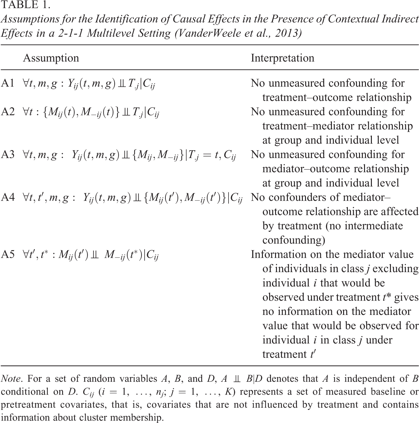
Note. For a set of random variables A, B, and D, A ╨ B|D denotes that A is independent of B conditional on D. C_ij (i = 1, …, n_j ; j = 1, …, K) represents a set of measured baseline or pretreatment covariates, that is, covariates that are not influenced by treatment and contains information about cluster membership.

A1, A2, A3, and A4 encode assumptions about the absence of unmeasured confounders for the relations between treatment, mediator, and/or outcome. They are called ignorability assumptions. Although these assumptions are rarely explicitly stated in educational research literature, it is key to realize that a randomized treatment only implies that Assumptions A1 and A2 hold, but does not guarantee that Assumption A3 is satisfied. One may indeed think of several factors at the student and/or class level that influence both the mediator and the outcome. Conditioning on such factors, contained in a set of baseline covariates C, may make the assumption of no unmeasured confounding for the mediator–outcome relationship more plausible. Assumption A4 is violated if some confounders of the M-Y relationship are affected by treatment. This assumption would for example not hold if training leads to a higher number of reading hours in the class, and the latter influences both the change in reading motivation and the change in reading. Assumption A5 states that information on the counterfactual M_ij (t′) provides no information on the counterfactual M_−ij (t*) conditional on observed covariates. This assumption will be violated if there is an unmeasured covariate, for instance, learning attitude of an individual student, which influences both the individual reading motivation and the motivation of other students in the class.

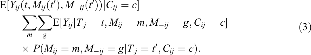
If the ignorability Assumptions A1, A2, A3, and A4 hold, the average counterfactual outcome $Y_{i j} (t, M_{i j} (t^{'}), M_{- i j} (t^{'}))$ conditional on C_ij is identified (VanderWeele et al., 2013) and is given by:

\begin{array}{l} E [Y_{i j} (t, M_{i j} (t^{'}), M_{- i j} (t^{'})) | C_{i j} = c] \\ = \sum_{m} \sum_{g} E [Y_{i j} | T_{. j} = t, M_{i j} = m, M_{- i j} = g, C_{i j} = c] \\ \times P (M_{i j} = m, M_{- i j} = g | T_{. j} = t^{'}, C_{i j} = c) . \end{array}

The expression in Equation 3 can be used to identify the NDE and the NIE.

If in addition Assumption A5 holds, then the average counterfactual outcome $Y_{i j} (t, M_{i j} (t^{'}), M_{- i j} (t^{*}))$ conditional on C_ij is identified (VanderWeele et al., 2013) and given by:

\sum_{m} \sum_{g} E [Y_{i j} | T_{. j} = t, M_{i j} = m, M_{- i j} = g, C_{i j}] \times P (M_{i j} = m | T_{. j} = t^{'}, C_{i j}) \times P (M_{- i j} = g | T_{. j} = t^{*}, C_{i j}) .

This expression can be used to identify the within indirect effect, Equation 2, and the contextual indirect effect, Equation 1.

Modeling Assumptions

Besides the above causal assumptions, we will also need to make modeling assumptions throughout the article. For ease of exposition, we start by considering the following simple data generating mechanisms for the mediator and outcome:

M_{i j} = β_{0} + β_{1} T_{. j} + β_{2} C_{i j} + u_{j} + r_{i j},

Y_{i j} = θ_{0} + θ_{1} T_{. j} + θ_{2} M_{i j} + θ_{3} M_{. j} + θ_{4} C_{i j} + u_{j}^{*} + ∊_{i j}^{*},

with M_.j equal to the class average of the mediator. We consider the outcome of student i in class j to depend on his or her own mediator but also on the class average M_.j, rather than the average of the classmates M_−ij . In groups of size 20 or more, M_−ij will be typically approximately equal to M_.j. Although M_ij and M_.j are not independent, we will further follow the view of VanderWeele et al. (2013) and replace M_−ij by the average of M_ij for all individuals in class j, M_.j, in the remainder of this article. This does not fundamentally change the estimators that we will discuss later (see the online Appendix B1, available at http://jeb.sagepub.com/supplemental) but simplifies the required calculations.

In Equations 5 and 6, the parameters β₀ and θ₀ represent the intercepts, β₁ and θ₁ represent the direct effect of treatment on, respectively, the mediator and outcome, θ₂ the effect of the individual mediator on outcome, θ₃ the effect of the class mean of the mediator on outcome, and β₂ and θ₄ the effect of (a vector of) measured baseline covariates (student- and/or class level-specific) on mediator and outcome. u_j , $u_{j}^{*}$ , r_ij and $∊_{i j}^{*}$ represent the upper-level and lower-level zero mean error terms, respectively, and each of them separately is assumed to be independent and identically distributed (across levels of i and j). Further, lower-level residuals are assumed to be independent of upper-level residuals.

Note that we allow unmeasured factors u_j such as teacher or class characteristics that influence both M_ij and M_.j. For example, if M_ij represents autonomous reading motivation of individual i in class j and M_.j the average autonomous motivation over all classmates, it is unlikely that those are independent, given the same teacher training. Furthermore, as it is often unlikely that all common causes of the mediator and outcome at the class level are measured, we will require that $u_{j}^{*} ╨ u_{j}$ . While Castellano et al. (2014) refer to such unmeasured common causes as Level 2 endogeneity, we use the term “unmeasured upper-level confounding” and make the following modeling assumption:

M1: Unmeasured upper-level confounders of the association between mediator and outcome exert an additive effect on both the mediator and the outcome, that is, their effects do not interact with treatment and/or mediator.

We do, however, assume that $∊_{i j}^{*} ╨ r_{i j}$ , implying that there is no unmeasured confounding for the mediator–outcome relationship at the lower level in line with Assumption A3. In the “Unmeasured Confounding of the M-Y Relationship” subsection, we propose a sensitivity analysis that will allow us to assess the impact of violations of the latter assumption on the estimation of indirect effects.

A second and third important modeling assumption implied by the data generating mechanisms in Equations 5 and 6 can be phrased as follows:

M2: There is no heterogeneity between classes in the effect of treatment on mediator and in the effect of treatment and mediator on outcome.

and

M3: There is no heterogeneity between individuals in the same class in the effect of treatment on mediator and in the effect of treatment and mediator on outcome.

In other words, we assume homogeneous effects across classes M2 and across individuals in the same class M3, given the observed data. The data generating mechanisms in Equations 5 and 6 do not allow for such moderation of the treatment effect by baseline covariates (neither at the student nor at the class level) for both mediator and outcome, as well as moderation of the mediator–outcome relationship, and assumes constant effects for all students in all classes. The fourth modeling assumption is:

M4: Treatment and mediator do not interact on the additive scale in their effect on the outcome.

For ease of exposition, we start from this simple setting without interactions, but later we show how to allow for such moderated mediation.

Derivation of Direct and Indirect Effects in Linear Models

We now derive the natural direct and indirect effects under the linear models in Equations 5 and 6 that obey Modeling Assumptions M1–M4. With a slight abuse of notation, let C_ij include u_j and $u_{j}^{*}$ in the assumptions in Table 1 (rationale explained below), then Assumptions A1–A4 are met under those models. In particular, using Equation 3, the NDE (under the linear models in Equations 5 and 6) equals,

E [Y_{i j} (1, M_{i j} (0), M_{. j} (0)) | C_{i j}] - E [Y_{i j} (0, M_{i j} (0), M_{. j} (0)) | C_{i j}] = θ_{1},

while the NIE equals

E [Y_{i j} (1, M_{i j} (1), M_{. j} (1)) | C_{i j}] - E [Y_{i j} (1, M_{i j} (0), M_{. j} (0)) | C_{i j}] = β_{1} (θ_{2} + θ_{3}) .

Interestingly, the direct and indirect effects do not depend on u_j and $u_{j}^{*}$ in this particular linear setting. Under models in Equations 5 and 6, Assumption A5 additionally holds, so we can also derive the natural contextual indirect effect,

E [Y_{i j} (1, M_{i j} (1), M_{. j} (1)) | C_{i j}] - E [Y_{i j} (1, M_{i j} (1), M_{. j} (0)) | C_{i j}] = β_{1} θ_{3},

and the natural within indirect effect:

E [Y_{i j} (1, M_{i j} (1), M_{. j} (0)) | C_{i j}] - E [Y_{i j} (1, M_{i j} (0), M_{. j} (0)) | C_{i j}] = β_{1} θ_{2} .

More details on these derivations can be found in the online Appendix B2 (available at http://jeb.sagepub.com/supplemental). Again, none of these conditional effects depend on u_j or $u_{j}^{*}$ in this linear setting, and marginal effects obtained by averaging over u_j or $u_{j}^{*}$ are thus identical. In the next section, we investigate under which conditions these effects are identified.

Methods for Multilevel Mediation Analysis

The Method of Pituch and Stapleton

The method of Pituch and Stapleton (2012), further abbreviated as PS method, considers two separate multilevel models:

M_{i j} = ζ_{0} + ζ_{1} T_{. j} + ζ_{2} C_{i j} + τ_{j} + υ_{i j},

Y_{i j} = λ_{0} + λ_{D E} T_{. j} + λ_{W I E} M_{i j} + λ_{C I E} M_{. j} + λ_{4} C_{i j} + τ_{j}^{*} + υ_{i j}^{*},

with $τ_{j}$ and $τ_{j}^{*}$ upper-level error terms and $υ_{i j}$ and $υ_{i j}^{*}$ lower-level error terms, all with mean zero and independent from the predictors in the model, $τ_{j}^{*} ╨ τ_{j}$ and $υ_{i j}^{*} ╨ υ_{i j}$ . Both random intercept models are fitted separately using restricted maximum likelihood estimation, hereby assuming normal distributions for error terms and random effects, to obtain estimators ${\hat{ζ}}_{1}$ , ${\hat{λ}}_{DE}$ , ${\hat{λ}}_{WIE}$ , and ${\hat{λ}}_{CIE}$ for the path coefficients of interest $ζ_{1}$ , $λ_{DE}$ , $λ_{WIE}$ , and $λ_{CIE}$ .

As shown in the right panel of Figure 1 (leaving out C_ij for clarity), the PS method aims to distinguish between the contextual indirect effect (estimated as ${\hat{ζ}}_{1} {\hat{λ}}_{CIE}$ ) and the individual indirect effect (estimated as ${\hat{ζ}}_{1} {\hat{λ}}_{WIE}$ ). Under the data generating models in Equations 5 and 6, and assuming $u_{j} ╨ u_{j}^{*}$ , it is easy to show that $E [{\hat{ζ}}_{1}] = β_{1}$ , $E [{\hat{λ}}_{DE}] = θ_{1}$ , $E [{\hat{λ}}_{WIE}] = θ_{2}$ , and $E [{\hat{λ}}_{CIE}] = θ_{3}$ in large samples. This method thus delivers asymptotically unbiased estimators for the direct and indirect effects of interest under the identification Assumptions A1 through A5 and Modeling Assumptions M1 through M4. In the remainder of this article, bias refers to asymptotic bias.

To unbiasedly estimate the contextual indirect and the direct effect separately, as one aims to do with the PS method, we thus require the strong assumption that $u_{j} ╨ u_{j}^{*}$ (the bias under violation of this independence assumption will be derived later). In the next section, we propose the ROD method, which uses a different parametrization and yields meaningful causal interpretations of the estimated parameter effects, even in the presence of unmeasured upper-level confounding for the mediator–outcome relationship.

The ROD Method

We here propose an alternative strategy to the PS method that effectively eliminates unmeasured upper-level confounding by applying cluster-mean centering (Castellano, Rabe-Hesketh, & Skrondal, 2014). Consider the data generating models in Equations 5 and 6, without the assumption that u_j and $u_{j}^{*}$ are independent. It is easy to see that:

Y_{i j} - Y_{. j} = θ_{2} (M_{i j} - M_{. j}) + θ_{4} (C_{i j} - C_{. j}) + (∊_{i j}^{*} - ∊_{. j}^{*}) .

Hence, by regressing the group-centered outcome (Y_ij−Y_.j) on the group-centered mediator (M_ij−M_.j) and baseline confounders (C_ij−C_.j), that is,

Y_{i j} - Y_{. j} = δ_{WIE} (M_{i j} - M_{. j}) + δ_{4} (C_{i j} - C_{. j}) + e_{i j},

unmeasured confounding at the group level is elegantly canceled out. This strategy thus identifies θ₂; even if $u_{j}$ and $u_{j}^{*}$ are not independent. An estimator for δ_WIE is obtained by fitting model in Equation 10 using ordinary least squares (OLS) regression. When moreover β₁ estimated using the same approach as PS and next multiplied by the just obtained estimator of δ_WIE, one obtains an unbiased estimate of the within indirect effect (β₁θ₂) while allowing for unmeasured M-Y confounding at the group level. Hence, the within indirect effect can be unbiasedly estimated under less stringent conditions. Indeed, Assumptions A3 and A5 can be weakened in the linear case with additive effects, in the sense that C_ij may include unmeasured upper-level confounders for the M-Y relationship that exert an additive effect on mediator and outcome. We refer to these weakened assumptions as Assumptions A3.B and A5.B.

Next, along the lines of Goetgeluk, Vansteelandt, and Goetghebeur (2008) and Loeys, Moerkerke, Raes, Rosseel, and Vansteelandt (2014), one may obtain an estimator of the effect of the treatment on the outcome not going through this individual mediator (Figure 2) by removing the effect of the individual mediator on the outcome and regressing this new outcome on the treatment:

Figure 2.

Second step of the regression of difference method: by subtracting δ_WIE M_ij of Y_ij we take away the edge between M_ij and Y_ij .

Y_{i j} - {\hat{δ}}_{WIE} M_{i j} = {δ^{'}}_{0} + δ_{DE} T_{. j} + ξ_{i j} .

An estimator for δ_DE, denoted as ${\hat{δ}}_{D E}$ , can be obtained using OLS under model in Equation 11. Following Moerkerke, Loeys, and Vansteelandt (2015), it can be shown that under data generating models in Equations 5 and 6, $E ({\hat{δ}}_{DE}) = θ_{1} + β_{1} θ_{3}$ , that is, a combination of the direct effect and the contextual indirect effect (see the online Appendix B3, available at http://jeb.sagepub.com/supplemental). Throughout this article, we will refer to this as the combined direct effect. While this combination of the direct and contextual indirect effect can be unbiasedly estimated when u_j and $u_{j}^{*}$ are dependent, the separate effects can only be unbiasedly estimated with the PS method under the assumption of no unmeasured M-Y confounding, Assumption A3. So the estimator of the combined direct effect is robust against upper-level M-Y confounding.

Since one fits Equations 9 and 11 consecutively, standard errors for ${\hat{δ}}_{WIE}$ and ${\hat{δ}}_{DE}$ are more difficult to obtain. Indeed, it is important to realize that when estimating $δ_{DE}$ and $δ_{WIE}$ , the standard error for ${\hat{δ}}_{DE}$ must account for the imprecision of ${\hat{δ}}_{WIE}$ . We will refer to the approach that ignores this uncertainty as the naive approach. For this latter approach, we have to use hierarchical modeling (e.g., random intercept model) to obtain standard errors for ${\hat{δ}}_{WIE}$ . To deal with the imprecision of ${\hat{δ}}_{WIE}$ when estimating the standard error of ${\hat{δ}}_{DE}$ , one can rely either on robust standard errors based on the sandwich estimator (Stefanski & Boos, 2002) or on bootstrap. The former provides consistent estimates of the covariance matrix for parameter estimates, even when the model is misspecified. The derivation of the standard errors for ${\hat{δ}}_{DE}$ and ${\hat{δ}}_{WIE}$ based on a robust sandwich estimator is shown in the online Appendix B4 (available at http://jeb.sagepub.com/supplemental), and its performance is assessed in the simulation study in the next section. In the simulations, we also consider two bootstrap approaches: bootstrapping of cases (Davison & Hinkley, 1997) and bootstrapping of residuals (Pituch & Stapleton, 2008). While the latter relies on the specified model to derive the (upper and lower) residuals, the former accounts for the hierarchical structure of the data by resampling on the class level. For the bootstrapping of cases, we use 95% percentile bootstrap confidence interval (CI), obtained by simply taking the 2.5th and 97.5th percentile of the bootstrap estimates as upper and lower bound. We will further refer to this approach as the nonparametric percentile-based bootstrap of cases (NPBS-C). It has been argued though that resampling of cases may not be very efficient when the number of classes is small (Davison & Hinkley, 1997). Pituch and Stapleton (2008) studied the performance of bootstrapping residuals for testing indirect effects in multilevel mediation models and found the bias-corrected parametric percentile bootstrap to perform among the best. We will refer to this method as the parametric percentile-based bootstrap of residuals (PPBS-R). In the parametric approach, one repeatedly draws samples from the estimated distribution of the residuals. For technical details on the implementation of the PPBS-R, we refer the interested reader to the five-step procedure and the additional bias adjustment described in that article. By considering percentile bootstrap, both the NPBS-C and the PPBS-R avoid assumptions on the distribution of the estimated quantity of interest, which may be particularly important when products of coefficients are involved such as for the indirect and combined direct effect. Pituch and Stapleton only studied the performance of different bootstrap procedures for the indirect effect, but we will use the PPBS-R here for all effects of interest in our setting.

The ROD method described above closely corresponds to the two steps of the Hausman–Taylor (HT) estimator introduced by Castellano et al. (2014) in the educational setting. Similar to our procedure but not specifically for a mediation context, the idea is to first eliminate the upper-level confounding by estimating the within effect of interest with a fixed effect estimator (Step 1) and next to consider the between-level effect that is appropriately adjusted for this within effect (Step 2). We refer the interested reader to appendix A of Castellano et al. (2014) for more technical details. The procedure for the HT estimator also produces valid standard errors. In the four steps of the procedure of the HT estimator, one obtains naive estimators in the first two steps, but next both parameters are reestimated simultaneously in the next two steps, so that the uncertainty in the estimate of δ_WIE is not ignored when estimating the standard error of ${\hat{δ}}_{DE}$ (Castellano et al., 2014). This procedure is implemented in the pht function in the plm R package (Croissant & Millo, 2008). Importantly, the ROD method is more easy to implement, as it simply relies on OLS for estimation and standard errors can be based on sandwich estimator.

Unmeasured Confounding of the M–Y Relationship

In this section, we obtain expressions for the bias of different estimators in the different methods under lower and upper-level confounding of the M-Y relationship. To this end, we consider an alternative formulation for the data generating mechanism models in Equations 5 and 6:

M_{i j} = β_{0} + β_{1} T_{. j} + u_{j} + r_{i j},

Y_{i j} = θ_{0} + θ_{1} T_{. j} + θ_{2} M_{i j} + θ_{3} M_{. j} + η u_{j} + {u^{'}}_{j} + ρ r_{i j} + ∊_{i j},

with now both ${u^{'}}_{j} ╨ u_{j}$ and $∊_{i j} ╨ r_{i j}$ . For ease of notation and calculations, we have dropped the baseline covariates C_ij from the models. Results can, however, easily be generalized to models containing C_ij . Parameters η and ρ capture unmeasured M-Y confounding at the upper level and lower level, respectively. This parametrization results in simple bias expressions for the ROD and PS estimators under such confounding, and therefore allows to derive relatively straightforward sensitivity analyses.

We first assess the bias of the estimator for δ_WIE in the model in Equation 10 of the ROD approach under data generating mechanisms in Equations 12 and 13. Replacing r_ij in Equation 13 by $M_{i j} - β_{0} - β_{1} T_{. j} - u_{j}$ (from Equation 12), one finds that:

Y_{i j} = (θ_{0} - ρ β_{0}) + (θ_{1} - ρ β_{1}) T_{j} + (θ_{2} + ρ) M_{i j} + θ_{3} M_{j} + η u_{j} + {u^{'}}_{j} - ρ u_{j} + ∊_{i j}

and Y_{. j} = (θ_{0} - ρ β_{0}) + (θ_{1} - ρ β_{1}) T_{j} + (θ_{2} + ρ) M_{. j} + θ_{3} M_{j} + η u_{j} + {u^{'}}_{j} - ρ u_{j} + ∊_{. j} .

The ROD approach thus yields:

Y_{i j} - Y_{. j} = (θ_{2} + ρ) (M_{i j} - M_{. j}) + ∊_{i j} - ∊_{. j},

and δ_WIE in the ROD approach will reflect the effect θ₂ + ρ under models in Equations 12 and 13 and hence, there is no bias under upper-level M-Y confounding (η ≠ 0).

We next develop a sensitivity analysis in the ROD framework that enables analysts to investigate the robustness of the within indirect effect estimator ${\hat{δ}}_{WIE}$ against violation of the no unmeasured M-Y confounding at the individual level (Assumption A3.B). More specifically, we will explore here how the estimated within indirect effect varies for a range of different values of the unknown ρ. Given a value of ρ, the parameter of interest θ₂ is then estimated by ${\hat{δ}}_{WIE} - ρ$ . Because ρ can take on any real value, we will rather use the correlation between the lower-level residual error terms in Equations 12 and 13 as a sensitivity parameter, that is, ρ* = cor(ρr_ij + ∊ _ij , r_ij ). This is similar in spirit to the sensitivity analysis proposed by Imai, Keele, and Tingley (2010) that is developed outside the multilevel context. In fact, we start with the same sensitivity parameter as Imai et al. (2010), but we decompose the error terms in such a way that we model the unmeasured confounding explicitly. Doing so, we obtain the simple bias expressions described above and we can propose a sensitivity analysis that is easier to generalize. It can easily be shown that:

ρ^{*} = \frac{ρ σ_{r}}{\sqrt{ρ^{2} σ_{r}^{2} + σ_{∊}^{2}}},

where $σ_{r}^{2}$ denotes the variance of r_ij and $σ_{∊}^{2}$ the variance of ∊ _ij . Using ρ* rather than ρ as sensitivity parameter, we can rewrite Equation 15:

ρ = \frac{ρ^{*}}{\sqrt{1 - ρ^{* 2}}} \frac{σ_{∊}}{σ_{r}} .

Upon noting that $var (∊_{i j}) = var (\frac{∊_{i j} - ∊_{. j}}{\sqrt{1 - \frac{1}{n_{j}}}})$ and $var (r_{i j}) = var (\frac{r_{i j} - r_{. j}}{\sqrt{1 - \frac{1}{n_{j}}}})$ , it follows that $σ_{∊}^{2}$ can be estimated in the ROD method as the sample variance of:

\frac{(Y_{i j} - Y_{. j}) - δ_{WIE} (M_{i j} - M_{. j})}{\sqrt{1 - \frac{1}{n_{j}}}},

where δ_WIE can be replaced by ${\hat{δ}}_{WIE}$ , and $σ_{r}^{2}$ as the sample variance of:

\frac{M_{i j} - M_{. j}}{\sqrt{1 - \frac{1}{n_{j}}}} .

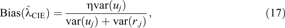
In practice, we proceed as follows. We first estimate δ_WIE, $σ_{r}^{2}$ , and $σ_{∊}^{2}$ at ρ* = 0. Next, we vary the level of ρ*, derive ρ using Equation 16, and estimate the within indirect effect for every value of ρ as ${\hat{ζ}}_{1} ({\hat{δ}}_{WIE} - ρ)$ . Note that the effect of the intervention on the mediator (β) can still be unbiasedly estimated by ${\hat{ζ}}_{1}$ from Equation 7 under unmeasured M-Y confounding at the lower level.

Next we consider the PS approach. In balanced designs, the estimators for the within indirect effect and the combined direct effect are mathematically equivalent to those obtained from the ROD method. In unbalanced designs, the within indirect effect is still mathematically equivalent but no longer the combined direct effect. This follows from the fact that the generalized least squares (GLS) estimator and OLS estimator for fixed effect parameters from linear mixed models are identical in balanced designs (Searle, Casella, & McCulloch, 2006, p. 160; Zyskind & Martin, 1969). Closed-form expressions for the GLS estimators from a linear mixed model with only a random intercept in unbalanced designs reveal that the GLS estimator for within-cluster effects (i.e., effects for cluster mean–centered predictors) is equal to the OLS estimator in unbalanced designs but no longer for between-cluster effects (Demidenko, 2013, Zyskind, 1967). The PS approach further disentangles the combined direct effect into the direct and contextual indirect effect but yields biased estimators for those effects in the presence of unmeasured upper-level M-Y confounding (under Assumption A3.B). We now quantify this bias. Assuming Equations 12 and 13 with η ≠ 0 but ρ = 0, the following expressions for the large sample bias of the PS estimators for θ₁ and θ₃ based on Equations 7 and 8 can be derived (see the online Appendix B5, available at http://jeb.sagepub.com/supplemental):

Bias ({\hat{λ}}_{CIE}) = \frac{η var (u_{j})}{var (u_{j}) + var (r_{. j})},

Bias ({\hat{λ}}_{DE}) = - \frac{η β_{1} var (u_{j})}{var (u_{j}) + var (r_{. j})} .

These expressions are derived under the assumption of the same number of students within each class, but the qualitative findings also hold as the number of students varies between classes. It is interesting to note that since the effect of the treatment on the mediator (i.e., β₁ under the data generating mechanisms in Equations 5 and 6) is still unbiasedly estimated by ${\hat{ζ}}_{1}$ , the estimator for the effect of the treatment not going through the individual mediator is unbiased, that is, $E ({\hat{λ}}_{D E} + {\hat{ζ}}_{1} {\hat{λ}}_{C I E}) = θ_{1} + β_{1} θ_{3}$ . As outlined in the online Appendix B5 (available at http://jeb.sagepub.com/supplemental), bias expression in Equation 17 can be used to develop a sensitivity analysis for the contextual indirect effect under the upper-level unmeasured confounding (Assumption A3.B). When unmeasured confounding is present at both levels, the total bias is obtained by adding the different expressions. A sensitivity analysis to check robustness against both types of confounding simultaneously may however become intractable.

Simulation Study

Using simulations, we assess the finite sample performance of the estimators of the direct and indirect effect estimators using the PS method and the ROD method and contrast the empirical bias under upper- or lower-level M-Y confounding with the above-derived bias expressions. We also compare the performance of six approaches to estimate the imprecision of the estimated within indirect effect and the combined direct effect. More specifically, we assess the empirical coverage of the 95% CIs of these effects using the naive approach, HT approach, the sandwich estimator, the NPBS-C, and the PPBS-R.

Using realistic assumptions about the number of classes and students, we explore four different scenarios using data generating mechanisms in Equations 12 and 13:

no M-Y confounding and a contextual indirect effect (η = 0, ρ = 0, and θ₃ = 0.3).

upper-level M-Y confounding but no contextual indirect effect (η = 0.2, ρ = 0, and θ₃ = 0).

upper-level M-Y confounding and contextual indirect effect (η = 0.2, ρ = 0, and θ₃ = 0.2).

upper- and lower level M-Y confounding and contextual indirect effect (η = 0.2, ρ = 0.4, and θ₃ = 0.2).

The following parameter choices were further made. The intraclass correlation coefficient for generating the mediator and the outcome in the clusters equals 0.2, β₁ = 0.1, θ₁ = 0.2, and θ₂ = 0.2. Sample size and group size vary as in Pituch and Stapleton (2012): 40 groups (gr = 40)/20 individuals (ind = 20), gr = 40, ind = 10 and gr = 20, ind = 20 and gr = 20, ind = 10. Note that similar results are obtained for unbalanced designs but not reported here.

Interest lies in estimation of the following effects:

the direct effect θ₁,

the within indirect effect β₁θ₂,

the contextual indirect effect β₁θ₃, and

the combined direct effect θ₁ + β₁θ₃.

Those four effects are estimated using the PS method (2012), while only the second and fourth are estimated using the ROD method. Each setting was repeated 1,000 times. R Version 3.1 was used to simulate and analyze the data (R Core Team 2015).

Results

Results are summarized in Table 2. Under setting (A), the PS method yields unbiased estimators of the direct $({\hat{λ}}_{DE})$ , the within $({\hat{ζ}}_{1} {\hat{λ}}_{WIE})$ , and the contextual indirect effect $({\hat{ζ}}_{1} {\hat{λ}}_{CIE})$ , as expected. The ROD method yields unbiased estimators of the within indirect effect $({\hat{ζ}}_{1} {\hat{δ}}_{WIE})$ and the combined direct effect $({\hat{δ}}_{DE})$ . As mentioned before, the estimators for the within indirect effect and the combined direct effect obtained by both methods are mathematically equivalent. This holds for this setting but also for all settings hereafter.

Table 2.

Results of the Simulation Studies When (A) no M-Y confounding is present, (B) upper-level M-Y Confounding Is Present but No Contextual Indirect Effect, (C) Upper-Level M-Y Confounding and Contextual Indirect Effect Are Present, and (D) Upper- And Lower-Level M-Y Confounding and Contextual Indirect Effect Are Present

			ROD Method				PS Method
N	G	θ₂	$B_{δ_{WIE}}$	${\hat{δ}}_{WIE}$	$B_{δ_{DE}}$	${\hat{δ}}_{DE}$	${\hat{ζ}}_{1}$	$B_{λ_{WIE}}$	${\hat{λ}}_{WIE}$	$B_{λ_{CIE}}$	${\hat{λ}}_{CIE}$	$B_{λ_{DE}}$	${\hat{λ}}_{DE}$	${\hat{λ}}_{DE} {+ \hat{ζ}}_{1} {\hat{λ}}_{CIE}$
Target parameter				θ₂		θ₁ + β₁θ₃	β₁		θ₂		θ₃		θ₁	θ₁ + β₁θ₃
True value				0.2		0.2 + 0.6θ₃	0.6		0.2		θ₃		0.2	0.2 + 0.6θ₃
						(A) η = ρ = 0 and θ₃ = 0.3
200	20	.2	0	.203	0	.380	.615	0	.203	0	.304	0	.190	.380
400	20	.2	0	.197	0	.384	.615	0	.197	0	.308	0	.196	.384
400	40	.2	0	.199	0	.386	.610	0	.199	0	.295	0	.207	.386
800	40	.2	0	.200	0	.376	.604	0	.200	0	.298	0	.198	.376
						(B) η = 0.2, ρ = 0, and θ₃ = 0
200	20	.2	0	.203	0	.196	.615	0	.203	.143	.148	−.086	.103	.196
400	20	.2	0	.197	0	.202	.615	0	.197	.167	.175	−.100	.094	.202
400	40	.2	0	.199	0	.204	.610	0	.199	.143	.138	−.086	.121	.204
800	40	.2	0	.200	0	.196	.604	0	.200	.167	.165	−.100	.098	.196
						(C) η = 0.2, ρ = 0, and θ₃ = 0.2
200	20	.2	0	.203	0	.320	.615	0	.203	.343	.348	−.086	.103	.320
400	20	.2	0	.197	0	.325	.615	0	.197	.367	.375	−.100	.094	.325
400	40	.2	0	.199	0	.326	.610	0	.199	.343	.338	−.086	.121	.326
800	40	.2	0	.200	0	.317	.604	0	.200	.367	.365	−.100	.098	.317
						(D) η = 0.2, ρ = 0.4, and θ₃ = 0.2
200	20	.2	.4	.603	−.24	.080	.601	.4	.603	−.143	.059	−.154	.042	.080
400	20	.2	.4	.599	−.24	.087	.595	.4	.599	−.167	.042	−.140	.064	.087
400	40	.2	.4	.599	−.24	.077	.615	.4	.599	−.143	.059	−.154	.043	.077
800	40	.2	.4	.601	−.24	.078	.602	.4	.601	−.167	.037	−.140	.055	.078

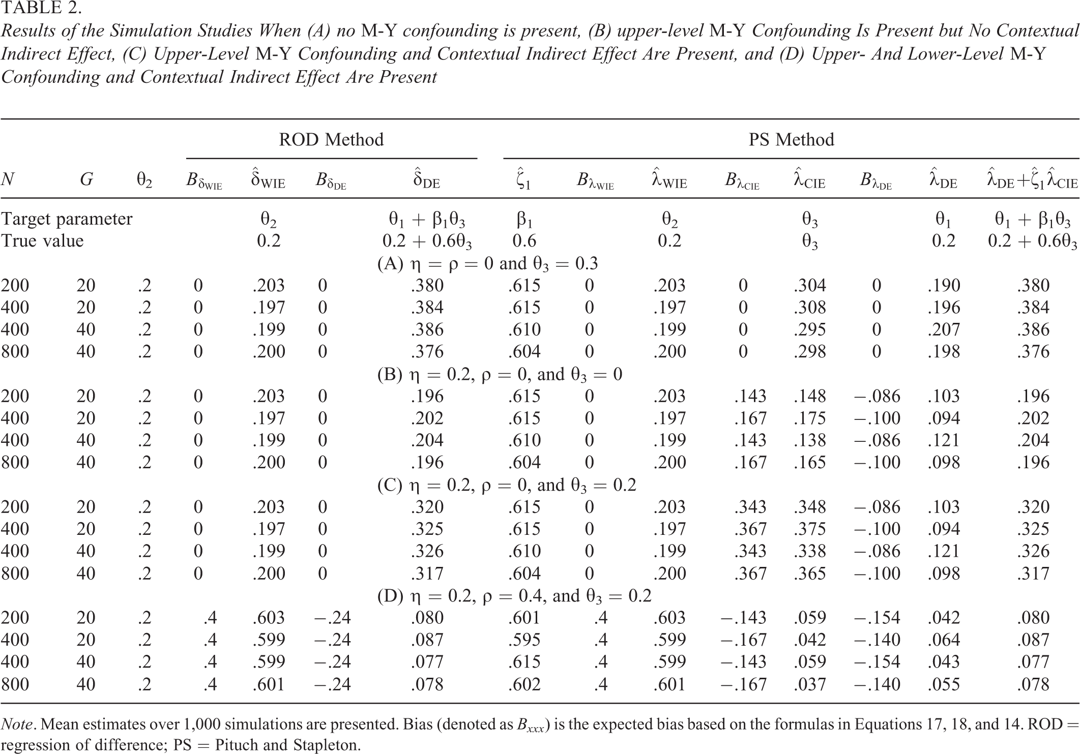
Note. Mean estimates over 1,000 simulations are presented. Bias (denoted as B_xxx ) is the expected bias based on the formulas in Equations 17, 18, and 14. ROD = regression of difference; PS = Pituch and Stapleton.

Under setting (B), the ROD method leads to unbiased estimators for the within indirect effect and the direct effect, that is, $E ({\hat{δ}}_{DE}) = θ_{1}$ , since there is no contextual indirect effect in this setting. For the PS method, we see, however, that both ${\hat{λ}}_{CIE}$ and ${\hat{λ}}_{DE}$ are biased estimators for θ₃ and θ₁. The method yields a nonexistent (positive) contextual indirect effect and a biased direct effect, and the observed bias for both estimators approximately corresponds to the expected bias based on Equations 17 and 18. This illustrates that the PS method cannot distinguish between a contextual indirect effect and unmeasured M-Y confounding at the group level.

Under setting (C), the estimator ${\hat{δ}}_{DE}$ unbiasedly estimates the combined direct effect. The PS method again yields biased estimates of the direct and contextual indirect effect.

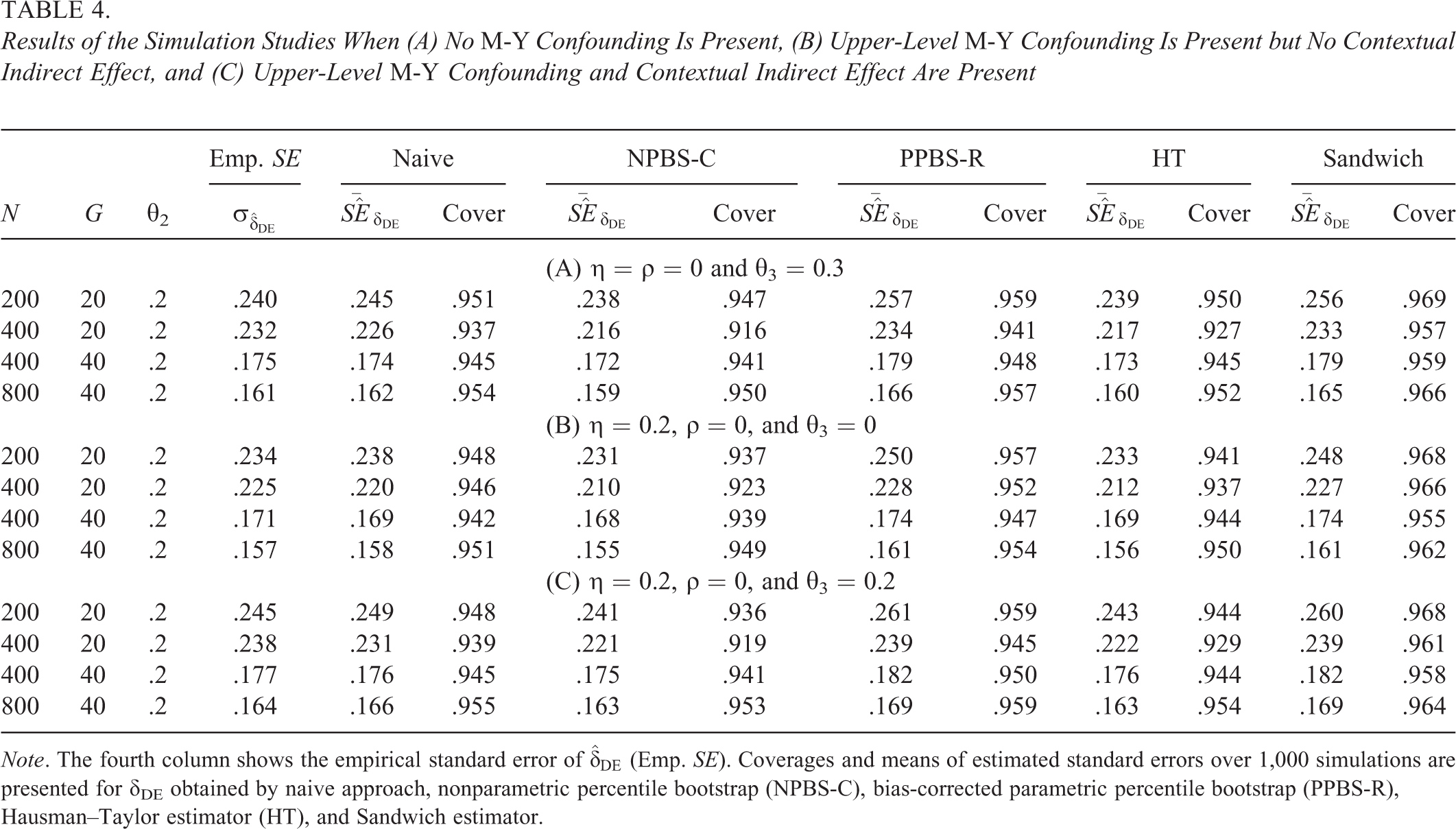
Under setting (D), all parameters of interest are estimated with bias under both approaches. We find that the bias for the estimators obtained by the PS method can be calculated as the sum of the bias formulas under upper- and lower-level confounding, that is, $Bias ({\hat{λ}}_{CIE}) = (17) + (23)$ and $Bias ({\hat{λ}}_{DE}) = (18) + (24)$ (see the online Appendix B5, available at http://jeb.sagepub.com/supplemental).

So far, we solely focused on the bias of the estimators from the ROD and PS methods. Next, we explore the coverages of the 95% CI of the ROD estimators and compare five different methods. Table 3 shows the mean of the estimated standard errors and the coverage of the 95% CI for δ_WIE under those five approaches. Scenario (D) was dropped, as the estimator for θ₂ is biased in this setting. The NPBS-C (using 2,000 bootstraps) tends to underestimate the variability of ${\hat{δ}}_{WIE}$ , resulting in undercoverage of the 95% CI, while the PPBS-R performs well, even in small sample sizes. The underestimation of the variability of the NPBS-C might be attributed to the small number of groups from which one can resample. Further, the naive approach and the HT approach perform well in terms of coverage. The sandwich estimator approach tends to show small undercoverage. Results for the combined direct effect are shown in Table 4. The results of ${\hat{δ}}_{DE}$ for both bootstrap approaches are roughly in line with those of ${\hat{δ}}_{WIE}$ . Further coverages for the HT approach are close to 95%, while the sandwich estimator-based approach turns out to be slightly conservative. Surprisingly, the coverage of 95% CI of the naive approach is also close to 95%. We also explore the coverage of the CI for the estimator of the within indirect effect. While the estimator of the within indirect effect is obtained as the product of estimators ${\hat{ζ}}_{1}$ and ${\hat{δ}}_{W I E}$ , its standard error is obtained using the Sobel formula $(s_{a b} = \sqrt{a^{2} s_{b}^{2} + s_{a}^{2} b^{2}})$ and Wald-type CI are constructed, except for the NPBS-C and PPBS-R which rely on the percentiles. Results are shown in Table B6 (see the online Appendix B6, available at http://jeb.sagepub.com/supplemental). We find that the coverage for the naive approach, the NPBS-C, the HT-estimator, and the sandwich estimator tend to be too low, while the coverages of the PPBS-R are close to 95%.

Table 3.

Results of the Simulation Studies When (A) No M-Y Confounding Is Present, (B) Upper-Level M-Y Confounding Is Present but No Contextual Indirect Effect, and (C) Upper-Level M-Y Confounding and Contextual Indirect Effect Are Present

			Emp. SE	Naive		NPBS-C		PPBS-R		HT		Sandwich
N	G	θ₂	$σ_{{\hat{δ}}_{WIE}}$	${\bar{\hat{S E}}}_{δ_{WIE}}$	Cover	${\bar{\hat{S E}}}_{δ_{WIE}}$	Cover	${\bar{\hat{S E}}}_{δ_{WIE}}$	Cover	${\bar{\hat{S E}}}_{δ_{WIE}}$	Cover	${\bar{\hat{S E}}}_{δ_{WIE}}$	Cover
						(A) η = ρ = 0 and θ₃ = 0.3
200	20	.2	.075	.071	.935	.071	.920	.076	.947	.075	.948	.074	.932
400	20	.2	.050	.050	.950	.048	.926	.052	.957	.052	.958	.051	.940
400	40	.2	.053	.050	.942	.051	.933	.053	.957	.053	.953	.052	.939
800	40	.2	.037	.035	.939	.035	.926	.036	.940	.036	.942	.036	.936
						(B) η = 0.2, ρ = 0, and θ₃ = 0
200	20	.2	.075	.071	.935	.071	.920	.076	.947	.075	.948	.074	.932
400	20	.2	.050	.050	.950	.048	.926	.052	.957	.052	.958	.051	.940
400	40	.2	.053	.050	.942	.051	.933	.053	.957	.053	.953	.052	.939
800	40	.2	.037	.035	.939	.035	.926	.036	.940	.036	.942	.036	.936
						(C) η = 0.2, ρ = 0, and θ₃ = 0.2
200	20	.2	.075	.071	.935	.071	.920	.076	.947	.075	.948	.074	.932
400	20	.2	.050	.050	.950	.048	.926	.052	.957	.052	.958	.051	.940
400	40	.2	.053	.050	.942	.051	.933	.053	.957	.053	.953	.052	.939
800	40	.2	.037	.035	.939	.035	.926	.036	.940	.036	.942	.036	.936

Note. The fourth column shows the empirical standard error of ${\hat{δ}}_{WIE}$ (Emp. SE). Coverages and means of estimated standard errors over 1,000 simulations are presented for δ_WIE obtained by naive approach, nonparametric percentile bootstrap (NPBS-C), bias-corrected parametric percentile bootstrap (PPBS-R), Hausman–Taylor estimator (HT), and Sandwich estimator.

Table 4.

			Emp. SE	Naive		NPBS-C		PPBS-R		HT		Sandwich
N	G	θ₂	$σ_{{\hat{δ}}_{DE}}$	${\bar{\hat{S E}}}_{δ_{DE}}$	Cover	${\bar{\hat{S E}}}_{δ_{DE}}$	Cover	${\bar{\hat{S E}}}_{δ_{DE}}$	Cover	${\bar{\hat{S E}}}_{δ_{DE}}$	Cover	${\bar{\hat{S E}}}_{δ_{DE}}$	Cover
						(A) η = ρ = 0 and θ₃ = 0.3
200	20	.2	.240	.245	.951	.238	.947	.257	.959	.239	.950	.256	.969
400	20	.2	.232	.226	.937	.216	.916	.234	.941	.217	.927	.233	.957
400	40	.2	.175	.174	.945	.172	.941	.179	.948	.173	.945	.179	.959
800	40	.2	.161	.162	.954	.159	.950	.166	.957	.160	.952	.165	.966
						(B) η = 0.2, ρ = 0, and θ₃ = 0
200	20	.2	.234	.238	.948	.231	.937	.250	.957	.233	.941	.248	.968
400	20	.2	.225	.220	.946	.210	.923	.228	.952	.212	.937	.227	.966
400	40	.2	.171	.169	.942	.168	.939	.174	.947	.169	.944	.174	.955
800	40	.2	.157	.158	.951	.155	.949	.161	.954	.156	.950	.161	.962
						(C) η = 0.2, ρ = 0, and θ₃ = 0.2
200	20	.2	.245	.249	.948	.241	.936	.261	.959	.243	.944	.260	.968
400	20	.2	.238	.231	.939	.221	.919	.239	.945	.222	.929	.239	.961
400	40	.2	.177	.176	.945	.175	.941	.182	.950	.176	.944	.182	.958
800	40	.2	.164	.166	.955	.163	.953	.169	.959	.163	.954	.169	.964

Note. The fourth column shows the empirical standard error of ${\hat{δ}}_{DE}$ (Emp. SE). Coverages and means of estimated standard errors over 1,000 simulations are presented for δ_DE obtained by naive approach, nonparametric percentile bootstrap (NPBS-C), bias-corrected parametric percentile bootstrap (PPBS-R), Hausman–Taylor estimator (HT), and Sandwich estimator.

Illustration

We now illustrate the ROD method and the sensitivity analysis with our motivating example. Interest lies in the effect of a need-supportive teaching style on change in reading frequency, and the extent to which this effect can be explained by a change in the students’ autonomous reading motivation. Before we start the data analysis, we discuss the plausibility of our causal assumptions. Assumptions A1 and A2 hold by randomization. If one is willing to assume that the effect of variables that affect both the reading frequency and the autonomous reading motivation (such as native language) is constant over time (i.e., at the pre- and postmeeting), such variables are no longer associated with the change in reading frequency and the change in autonomous reading motivation. By looking at the change, one can thus allow for unmeasured confounders that have a time-constant effect. However, if there are additional unmeasured covariates which have a different effect on pre- and postmeasurements of mediator and outcome, Assumption A3 would still be violated. Assumption A4 requires that there are no variables (such as the number of reading hours in the class) that depend on the need-supportive teaching style and that are associated with the change in reading frequency and the change in autonomous reading motivation, while Assumption A5 requires that the potential motivation of an individual student under some exposure is independent from the potential motivation of his or her friends under an assumed exposure in the same class. While both assumptions may not hold unconditionally, it is reasonable to assume that both assumptions may still hold conditional on unobserved class characteristics (such as the atmosphere in the class). That is sufficient to still identify the within indirect effect, provided that additive effects of these unmeasured class characteristics can be assumed. Further, it should be noted that schools are geographically separated but that in some schools, more than one class participated in this study, which may imply that the “no interference between classes” assumption may not fully hold. If part of the effect of the intervention on reading frequency is mediated by the reading motivation in other classrooms (hereby assuming an additive effect), but we ignore this and consider only the effect mediated through a child’s own classroom, then the direct effect will capture both the true NDE and the between-classes spillover-mediated effect (VanderWeele et al., 2013). As the ROD method only aims to disentangle the within indirect effect and the remaining “combined” direct effect, it is not impacted by violation of the no interference between classes assumption.

The total effect of the intervention on reading frequency, obtained by using a linear mixed model for the change in reading frequency with a fixed effect for intervention and a random intercept for each class, equals 0.093 (95% CI [−0.032, 0.217]). In other words, students of the treatment group have a change in reading frequency which lies 0.093 units above the change in the control group. Given that reading frequency is measured on a 4-point Likert-type scale, this difference is rather small and corresponds to approximately a 0.16 standard deviation increase. Interestingly, a −0.079 decrease and a 0.014 increase in reading frequency were observed in the control and intervention condition, respectively. In the traditional causal steps approach of the Baron and Kenny (1986) framework for mediation, a significant test for the total effect is considered a prerequisite for the test for the indirect effect. However, several scholars (Loeys, Moerkerke, & Vansteelandt, 2015; Shrout & Bolger, 2002) have argued that when primary interest lies in the mediation effect, the need for a significant total effect may be abandoned. We therefore continue to disentangle this nonsignificant total effect. Analyzing the data using the ROD method leads to a significant within indirect effect of training on reading frequency through autonomous reading motivation (0.048, 95% CI [0.010, 0.086]). Further, the estimate for the combined direct effect (δ_DE) is 0.042 (95% CI [−0.085, 0.170]) and is statistically nonsignificant (95% CI for the within indirect effect and the combined direct effect are based on the sandwich estimator). These estimates indicate that treatment leads to a higher change in reading frequency through the change of individual autonomous reading motivation (effect of 0.048) and to a higher change in reading frequency through the combination of all other paths (effect of 0.042). Again, these effects are rather small, given the 4-point Likert-type scale of reading frequency. We also analyze the data with the PS method. We find the same estimate and CI for the within indirect effect of training on reading frequency (0.048, 95% CI [0.012, 0.089], based on PPBS-R). The contextual indirect effect (0.043, 95% CI [−0.005, 0.119]) and the direct effect (−0.002, 95% CI [−0.120, 0.116]) are not statistically significant. It should be noted that these estimated effects rely on the absence of upper-level M-Y confounding. If we calculate the combined direct effect as the sum of the two latter effects, we obtain a similar but not identical estimate as the one obtained by the ROD method (0.042, 95% CI [−0.080, 0.153]).

While the ROD method and the PS method yield an unbiased estimator for the within indirect effect with unmeasured M-Y confounding at the class level (Assumption A3.B), this no longer holds in the presence of such confounding at the student level. As there might still be unmeasured common causes of change in autonomous reading motivation and change in reading frequency at the individual level, over and beyond such common causes at the group level, we perform a sensitivity analysis as outlined in the previous section. Figure 3 presents the results of the sensitivity analysis. For negative values of ρ*, the within indirect effect remains statistically significant. However, in this study, negative values are less realistic, given that one may expect that unmeasured common causes would impact change in autonomous reading motivation and change in reading frequency in the same direction. For instance, the distance between home and closest public library, which was unmeasured, may have an impact on reading motivation and on reading frequency. For positive values of ρ*, the indirect effect decreases with increasing ρ* becomes nonsignificant for ρ* > 0.23 and equals 0 when ρ* = 0.29. For very large values of ρ*, the indirect effect is again statistically significant but negative. However, we expect ρ* to be relatively small in our study. Indeed, as noted before, by studying the change in autonomous motivation and reading frequency rather than the posttest measurements, effects of potential confounders for autonomous motivation and reading frequency that are constant over time are canceled out. As an example, consider parent commitment, which was measured in this study. While parent commitment is strongly correlated with posttest autonomous motivation and reading frequency (correlation = .33 and .48, respectively), it is weakly correlated with the change from baseline in those measures (correlation = .09 and .14). The latter correlations imply a sensitivity parameter value equal to .01, and an analysis that explicitly adjusted for parent commitment indeed had a negligible impact on the within indirect effect. Although we cannot preclude confounding of the relation between change in autonomous motivation and change in reading frequency at the individual level, we thus conclude that for (expected) small positive correlations, the positive indirect effect is still significant but for (rather unexpected) moderate positive correlations, it would no longer be statistically significant.

Figure 3.

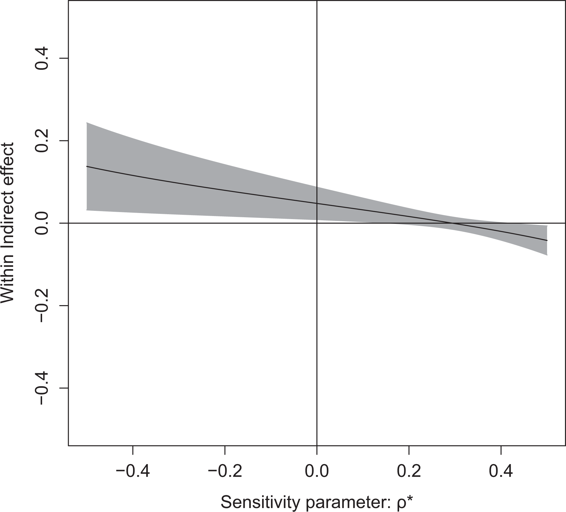
Effect of teacher training on reading frequency that is mediated by autonomous reading motivation and the individual level (with corresponding 95% confidence interval) for a range of different sensitivity parameters, ρ*.

Estimation of Indirect Effects in the Presence of Interactions

In practice, it is not always realistic to assume that there are no interactions between treatment, mediator, and/or covariates. For illustrative purposes, we will focus here on a setting with a treatment–mediator interaction (which implies that Modeling Assumption M4 is no longer necessary), and instead of models in Equations 5 and 6 consider the following set of data generating models (with C_ij dropped for clarity):

M_{i j} = β_{0} + β_{1} T_{. j} + u_{j} + r_{i j},

Y_{i j} = θ_{0} + θ_{1} T_{. j} + θ_{2} M_{i j} + θ_{3} M_{. j} + θ_{4} T_{. j} M_{i j} + θ_{5} T_{. j} M_{. j} + {u^{'}}_{j} + ∊_{i j},

with ∊ _ij ╨ r_ij , but not necessarily ${u^{'}}_{j} ╨ u_{j}$ . In the presence of such T-M interaction, we first need to extend our definitions of causal effects. The natural direct and indirect effects we defined before are referred to as “pure direct effect” and “total indirect effect” by Robins and Greenland (1992). For the NDE, we compared average outcome under treatment versus control, in both cases setting the individual and group-averaged mediator to what it would have been in the absence of treatment (i.e., “the pure direct effect”). We might instead compare treatment to control, now in both cases setting the mediators to the level they would have taken under treatment (i.e., “the total direct effect”). Similarly, we distinguish the “pure” from “total” indirect effect. In the absence of T-M interactions, the pure and total (in-)direct effects are the same. The total effect can be decomposed either into a total indirect effect and a pure direct effect or into a total direct effect and a pure indirect effect. Recently, VanderWeele (2013) derived a three-way decomposition of the total effect in a pure direct, pure indirect, and interactive-mediated effect. The latter is a counterfactual measure of additive interaction. In Table 5, we extend those definitions to allow for spillover effects and also decompose the total effect into the sum of these three effects. The pure indirect effect and the interactive-mediated effect are then further decomposed into a within and contextual part. Under data generating mechanisms in Equations 19 and 20, the identification assumptions are met, and corresponding causal effects are shown in the last column of Table 5.

Table 5.

Counterfactual Definitions of Causal Effects in the Presence of T-M Interactions in a 2-1-1 Multilevel Setting

Causal Effect	Counterfactual Definition	Value
Total	$E [Y_{i j} (1, M_{i j} (1), M_{. j} (1))] - E [Y_{i j} (0, M_{i j} (0), M_{. j} (0))]$
Pure direct	$E [Y_{i j} (1, M_{i j} (0), M_{. j} (0))] - E [Y_{i j} (0, M_{i j} (0), M_{. j} (0))]$	$θ_{1} + (θ_{4} + θ_{5}) β_{0}$
Pure indirect	$E [Y_{i j} (0, M_{i j} (1), M_{. j} (1))] - E [Y_{i j} (0, M_{i j} (0), M_{. j} (0))]$	$β_{1} (θ_{2} + θ_{3})$
Interactive mediated	$E [Y_{i j} (1, M_{i j} (1), M_{. j} (1))] - E [Y_{i j} (1, M_{i j} (0), M_{. j} (0))]$ $- E [Y_{i j} (0, M_{i j} (1), M_{. j} (1))] + E [Y_{i j} (0, M_{i j} (0), M_{. j} (0))]$	$β_{1} (θ_{4} + θ_{5})$
Pure within indirect	$E [Y_{i j} (0, M_{i j} (1), M_{. j} (1))] - E [Y_{i j} (0, M_{i j} (0), M_{. j} (1))]$	β₁θ₂
Pure contextual indirect	$E [Y_{i j} (0, M_{i j} (0), M_{. j} (1))] - E [Y_{i j} (0, M_{i j} (0), M_{. j} (0))]$	β₁θ₃
Interactive within mediated	$E [Y_{i j} (1, M_{i j} (1), M_{. j} (1))] - E [Y_{i j} (1, M_{i j} (0), M_{. j} (1))]$ $- E [Y_{i j} (0, M_{i j} (1), M_{. j} (1))] + E [Y_{i j} (0, M_{i j} (0), M_{. j} (1))]$	β₁θ₄
Interactive contextual mediated	$E [Y_{i j} (1, M_{i j} (0), M_{. j} (1))] - E [Y_{i j} (1, M_{i j} (0), M_{. j} (0))]$ $- E [Y_{i j} (0, M_{i j} (0), M_{. j} (1))] + E [Y_{i j} (0, M_{i j} (0), M_{. j} (0)]$	β₁θ₅

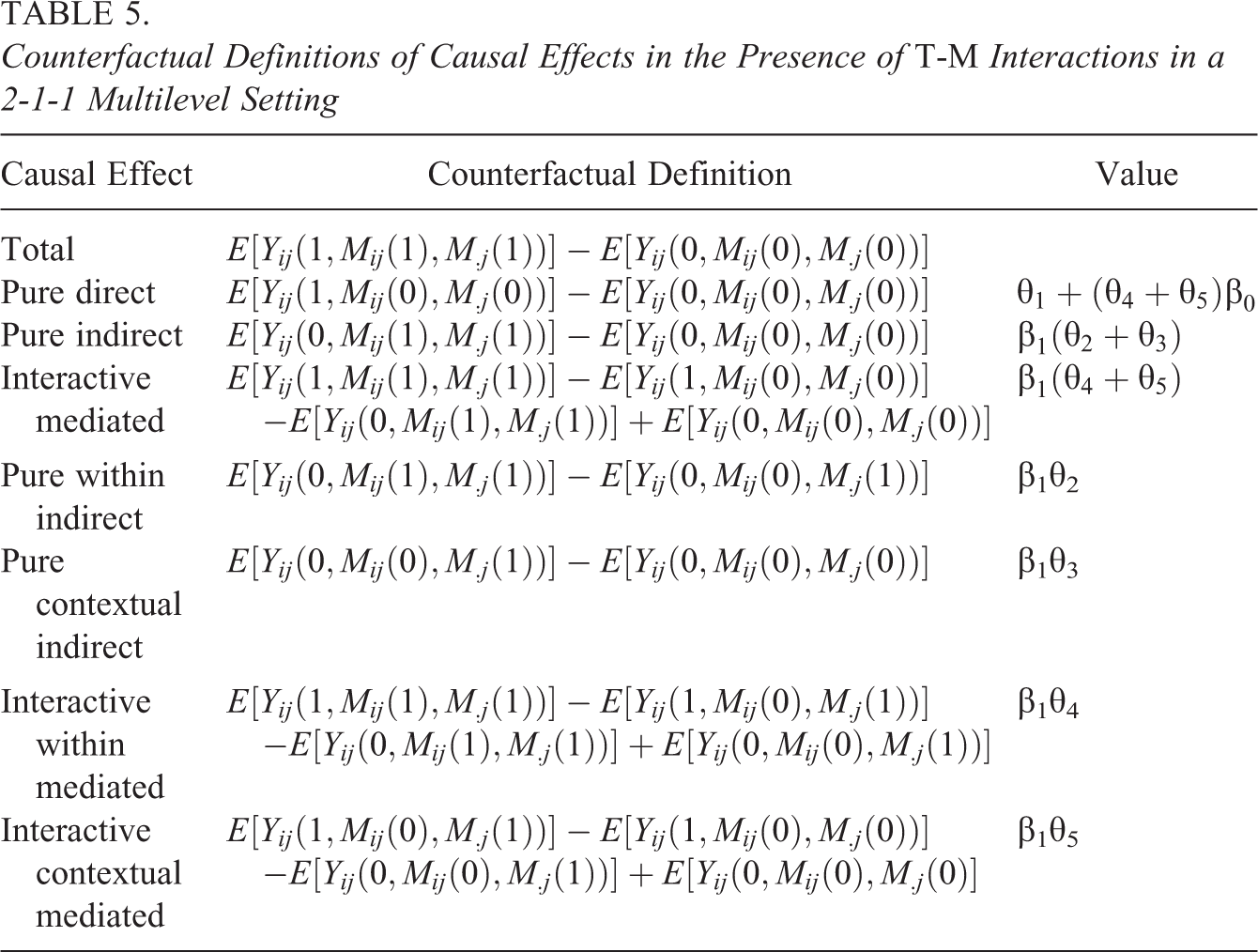
Upon noting that under the model in Equation 20:

Y_{i j} - Y_{. j} = θ_{2} (M_{i j} - M_{. j}) + θ_{4} T_{. j} (M_{i j} - M_{. j}) + (∊_{i j} - ∊_{. j}),

it is easy to see that using the ROD approach, whereby one regresses the group-centered outcomes on the group-centered mediators and its interaction with treatment, one can easily obtain unbiased estimators of the pure within indirect effect and the interactive within-mediated effect. Denoting those estimators by ${\hat{δ}}_{WIE}$ and ${\hat{δ}}_{WIA}$ , we can remove the effect of the individual mediator (M_ij ) on the outcome and regress this new outcome on treatment, that is,

Y_{i j} - {\hat{δ}}_{WIE} M_{i j} - {\hat{δ}}_{WIA} T_{. j} M_{i j} = {δ^{'}}_{0} + δ_{DE} T_{. j} + ξ_{i j} .

Using similar arguments as before, it can be shown that ${\hat{δ}}_{DE}$ is an unbiased estimator of the sum of the pure indirect effect, the pure contextual indirect effect, and the interactive contextual-mediated effect.

Discussion and Conclusion

In this article, we have clarified under which assumptions causal direct, within, and contextual indirect effects can be identified in the 2-1-1 setting. When focusing on the linear setting in particular, we have shown that the within indirect effect can still be identified when additionally allowing for unmeasured common causes of mediator and/or outcome at the class level that have an additive effect. This result extends the findings of Castellano et al. (2014) to the mediation setting. Similar to their fixed effects approach, we proposed the ROD method as an easy-to-implement strategy to estimate the within indirect effect under those assumptions. The second step of our approach also straightforwardly yields an unbiased estimator of the “combined direct effect,” which we defined as the sum of the direct effect and the contextual indirect effect. While neither of the latter two can be identified under upper-level M-Y confounding, their sum is identified under our set of assumptions. In contrast, the PS method aims to estimate those two effects separately, but as shown in this article, stronger assumptions are required to this end. As the within indirect effect can no longer be identified under unmeasured lower-level M-Y confounding, we introduced a sensitivity analysis that allows analysts to assess the robustness of that effect against the presence of such confounders. Similarly, a sensitivity analysis can be used to check the robustness of estimates for the contextual indirect effect of the PS approach in the presence of upper-level confounding. Of note, the ROD approach and the PS approach yield mathematically equivalent estimators for the within indirect effect and the combined direct effect in balanced designs. In unbalanced designs, only the within indirect effect is exactly the same, but simulations (results not shown) revealed negligible differences for the combined direct effect estimators of the two approaches when the linearity and normality assumptions hold.

We have restricted our study to the linear multilevel setting with continuous mediators and outcomes. This type of model is most common in educational research. Mediation analysis from a causal perspective in the more general multilevel setting has received little attention so far in the literature (Preacher, 2015). One of the rare exceptions is the R mediation package (Tingley, Yamamoto, Hirose, Keele, & Imai, 2014). This approach relies on the mediation formula (Imai, Keele, & Tingley, 2010) and will yield unbiased estimators for the direct effect and within indirect effects under the identification Assumptions A1 through A5 outlined in this article when models for mediator and outcome are correctly specified but may suffer from the same weaknesses as the PS method under unmeasured upper-level M-Y confounding (i.e., under Assumptions 3.B). Moreover, the easy-to-implement sensitivity analysis assessing the robustness against unmeasured M-Y confounding that can be performed with the mediation package in the simple setting with independent observations is not yet available in the hierarchical setting. Throughout, we have primarily focused on models with no interactions but gave an introduction on how the proposed ROD method can be elegantly extended to allow for M-Y interactions for example. Researchers should be aware that properties and interpretation of the different estimators rely on the assumption that models are correctly specified. Throughout the article, we assume for example that, conditional on covariates, causal effects are constant across students. When interactions are omitted, for instance, between treatment and covariates, the obtained effects are still indicative as average effects across covariate levels (Liu & Gustafson, 2008), provided that appropriate adjustment for confounders of the M-Y relationship is made.

Another important assumption made in this article is the absence of measurement error. It is well known that, similar to unmeasured confounding, measurement error in the mediator and/or outcome may introduce bias in the direct and indirect effect estimators (Cole & Preacher, 2014; Hoyle & Kenny, 1999; Ledgerwood & Shrout, 2011). Multilevel structural equation modeling (MSEM) offers much flexibility in terms of including latent variables and accounting for measurement error for upper-level covariates (Preacher, Zhang, & Zyphur, 2011). As Lüdtke et al. (2008) pointed out, the appropriateness of multilevel latent covariate or multilevel manifest covariate (MMC) approaches, which treat class-level constructs as latent and observed, respectively, depends on the research question and the nature of the upper-level construct under study. For example, if all students within a class are asked to rate the autonomous motivation of their class as a whole or his or her own autonomous motivation, respectively, the aggregated upper-level construct may be considered as a reflective or formative construct, respectively. Treating the class average motivation as observed, the MMC approach may result in biased estimates of contextual effects for the former. More importantly though, the within effect that we are particularly interested in can still be unbiasedly estimated for either type of the two constructs. Note that throughout the simulation studies, we did not analyze the data with MSEM, because under the scenario of no measurement error the method yields on average the same estimates as the approach of PS, but with more imprecision (Lüdtke et al., 2008).

Finally, in the cluster randomized trials discussed here, only two levels were considered: the student and the class level. However, in a study where schools are randomly assigned to instructional methods, multiple teachers within a given school may be involved. If the student outcome is of interest and each teacher is responsible for a single class, three levels would have to be considered: student, class, and school. While methods are available for the analysis of such three-level data (Pituch, Murphy, & Tate, 2009; Preacher, 2011), the identification assumptions for the different causal effects of interest in such setting remain to be clarified.

Footnotes

Declaration of Conflicting Interests

The authors declared no potential conflicts of interest with respect to the research, authorship, and/or publication of this article.

Funding

The computational resources (Stevin Supercomputer Infrastructure) and services used in this work were provided by the VSC (Flemish Supercomputer Center), funded by Ghent University, the Hercules Foundation and the Flemish Government - department EWI. The authors would like to thank the Flemish Research Council (FWO) (Grant G.0111.12).

Supplemental Material

The online appendices are available at

References

Baron

R. M.

Kenny

D. A.

(1986). The moderator-mediator variable distinction in social psychological research: Conceptual, strategic, and statistical considerations. Journal of Personality and Social Psychology, 51, 1173–1182. doi:10.1037/0022-3514.51.6.1173

Castellano

K. E.

Rabe-Hesketh

Skrondal

(2014). Composition, context, and endogeneity in school and teacher comparisons. Journal of Educational and Behavioral Statistics, 39, 333–367. doi:10.3102/1076998614547576

Cole

D. A.

Preacher

K. J.

(2014). Manifest variable path analysis: Potentially serious and misleading consequences due to uncorrected measurement error. Psychological Methods, 19, 300–315. doi:10.1037/a0033805

Croissant

Millo

(2008). Panel data econometrics in R: The plm package. Journal of Statistical Software, 27. Retrieved from http://th.archive.ubuntu.com/cran/web/packages/plm/vignettes/plm.pdf

Davison

A. C. A. C.

Hinkley

D. V.

(1997). Bootstrap methods and their application. Cambridge, England: Cambridge University Press.

Demidenko

(2013). Mixed models: Theory and applications with r. Hoboken, NJ: John Wiley. doi:10.1002/9781118651537

De Naeghel

Van Keer

Vansteenkiste

Haerens

Aelterman

(in press). Promoting elementary school students autonomous reading motivation: Effects of a teacher professional development workshop. Journal of Educational Research, in press.

De Naeghel

Van Keer

Vansteenkiste

Rosseel

(2012). The relation between elementary students’ recreational and academic reading motivation, reading frequency, engagement, and comprehension: A self-determination theory perspective. Journal of Educational Psychology, 104, 1006–1021. doi:10.1037/a0027800

Goetgeluk

Vansteelandt

Goetghebeur

(2008). Estimation of controlled direct effects. Journal of the Royal Statistical Society Series B: Statistical Methodology, 70, 1049–1066. doi:10.1111/j.1467-9868.2008.00673.x

10.

Hausman

J. A.

Taylor

W. E.

(1981). Panel data and unobservable individual effects. Econometrica, 49, 1377–1398. doi:10.2307/1911406

11.

Hong

Raudenbush

S. W.

(2006). Evaluating kindergarten retention policy. Journal of the American Statistical Association, 101, 901–910. doi:10.1198/016214506000000447

12.

Hong

Raudenbush

S. W.

(2008). Causal inference for time-varying instructional treatments. Journal of Educational and Behavioral Statistics, 33, 333–362. doi:10.3102/1076998607307355

13.

Hoyle

R. H.

Kenny

D. A.

(1999). Sample size, reliability, and tests of statistical mediation. In Hoyle

(Ed.), Statistical strategies for small sample research (pp. 195–222). Thousand Oaks, CA: Sage.

14.

Imai

Keele

Tingley

(2010). A general approach to causal mediation analysis. Psychological Methods, 15, 309–334. doi:10.1037/a0020761

15.

Krull

J. L.

Mackinnon

D. P.

(2001). Multivariate behavioral multilevel modeling of individual and group level mediated effects. Multivariate Behavioral Research, 36, 249–277. doi:10.1207/S15327906MBR3602

16.

Ledgerwood

Shrout

P. E.

(2011). The trade-off between accuracy and precision in latent variable models of mediation processes. Journal of Personality and Social Psychology, 101, 1174–1188. doi:10.1037/a0024776

17.

Liu

Gustafson

(2008). On average predictive comparisons and interactions. International Statistical Review, 76, 419–432. doi:10.1111/j.1751-5823.2008.00056.x

18.

Loeys

Moerkerke

Raes

Rosseel

Vansteelandt

(2014). Estimation of controlled direct effects in the presence of exposure-induced confounding and latent variables. Structural Equation Modeling: A Multidisciplinary Journal, 21, 396–407. doi:10.1080/10705511.2014.915372

19.

Loeys

Moerkerke

Vansteelandt

(2015). A cautionary note on the power of the test for the indirect effect in mediation analysis. Frontiers in Psychology, 5, 1–8. doi:10.3389/fpsyg.2014.01549

20.

Lüdtke

Marsh

H. W.

Robitzsch

Trautwein

Asparouhov

Muthén

(2008). The multilevel latent covariate model: A new, more reliable approach to grouplevel effects in contextual studies. Psychological Methods, 13, 203–229. doi:10.1037/a0012869

21.

MacKinnon

(2008). Introduction to statistical mediation analysis. New York, NY: Taylor & Francis Group.

22.

Moerkerke

Loeys

Vansteelandt

(2015). Structural equation modeling versus marginal structural modeling for assessing mediation in the presence of post-treatment confounding. Psychological Methods, 20, 204–220. doi:10.1037/a0036368

23.

Nagengast

Marsh

H. W.

(2012). Big fish in little ponds aspire more: Mediation and cross-cultural generalizability of school-average ability effects on self-concept and career aspirations in science. Journal of Educational Psychology, 104, 1033–1053. doi:10.1037/a0027697

24.

Pearl

(2001). Direct and indirect effects. In Breese

Koller

(Eds.), Proceedings of the seventeenth conference on uncertainty in artificial intelligence (pp. 411–420). San Francisco, CA: Morgan Kaufmann.

25.

Pearl

(2014). Interpretation and identification of causal mediation. Psychological Methods, 19, 459–481. doi:10.1037/a0036434

26.

Pituch

K. A.

Murphy

D. L.

Tate

R. L.

(2009). Three-level models for indirect effects in school- and class-randomized experiments in education. The Journal of Experimental Education, 78, 60–95. doi:10.1080/00220970903224685

27.

Pituch

K. A.

Stapleton

L. M.

(2008). The performance of methods to test upper-level mediation in the presence of nonnormal data. Multivariate Behavioral Research, 43, 237–267. doi:10.1080/00273170802034844

28.

Pituch

K. A.

Stapleton

L. M.

(2012). Distinguishing between cross- and cluster-level mediation processes in the cluster randomized trial. Sociological Methods & Research, 41, 630–670. doi:10.1177/0049124112460380

29.

Preacher

K. J.

(2011). Multilevel SEM strategies for evaluating mediation in three-level data. Multivariate Behavioral Research, 46, 691–731. doi:10.1080/00273171.2011.589280

30.

Preacher

K. J.

(2015). Advances in mediation analysis: A survey and synthesis of new developments. Annual Review of Psychology, 66, 825–852. doi:10.1146/annurev-psych-010814-015258

31.

Preacher

K. J.

Zhang

Zyphur

M. J.

(2011). Alternative methods for assessing mediation in multilevel data: The advantages of multilevel SEM. Structural Equation Modeling: A Multidisciplinary Journal, 18, 161–182. doi:10.1080/10705511.2011.557329

32.

Preacher

K. J.

Zyphur

M. J.

Zhang

(2010). A general multilevel SEM framework for assessing multilevel mediation. Psychological Methods, 15, 209–233. doi:10.1037/a0020141

33.

Raudenbush

S. W.

Willms

(1995). The estimation of school effects. Journal of Educational and Behavioral Statistics, 20. Retrieved from http://jeb.sagepub.com/content/20/4/307.short

34.

R Core Team. (2015). R: A language and environment for statistical computing [Computer software manual]. Vienna, Austria. Retrieved from http://www.R-project.org/

35.

Robins

J. M.

Greenland

(1992). Identifiability exchangeability effects for direct and indirect effects. Epidemiology, 3, 143–155. doi:10.1097/00001648-199203000-00013

36.

Rubin

D. B.

(1976). Inference and missing data. Biometrika, 63, 581–592. doi:10.1093/biomet/63.3.581

37.

Rubin

D. B.

(1980). Comment on: “Randomization analysis of experimental data in the Fisher randomization test” by D. Basu. Journal of the American Statistical Association, 75, 591–593. doi:10.1080/01621459.1980.10477517

38.

Searle

S. R.

Casella

McCulloch

C. E.

(2006). Variance components (Vol. 391). New York, NY: John Wiley.

39.

Shrout

P. E.

Bolger

(2002). Mediation in experimental and nonexperimental studies: New procedures and recommendations. Psychological Methods, 7, 422–445. doi:10.1037//1082-989X.7.4.422

40.

Stefanski

L. A.

Boos

D. D.

(2002). The calculus of m-estimation. The American Statistician, 56, 29–38. doi:10.1198/000313002753631330

41.

Tchetgen

E. J. T.

VanderWeele

T. J.

(2012). On causal inference in the presence of interference. Statistical Methods in Medical Research, 21, 55–75. doi:10.1177/0962280210386779

42.

Tingley

Yamamoto

Hirose

Keele

Imai

(2014). Mediation: R package for causal mediation analysis. Journal of Statistical Software, 59, 1–38. Retrieved from http://www.jstatsoft.org/v59/i05/

43.

VanderWeele

T. J.

(2008). Ignorability and stability assumptions in neighborhood effects research. Statistics in Medicine, 27, 1934–1943. doi:10.1002/sim

44.

VanderWeele

T. J.

(2010). Direct and indirect effects for neighborhood-based clustered and longitudinal data. Sociological Methods & Research, 38, 515–544. doi:10.1177/0049124110366236

45.

VanderWeele

T. J.

(2013). A three-way decomposition of a total effect into direct, indirect, and interactive effects. Epidemiology, 24, 224–232. doi:10.1097/EDE.0b013e318281a64e

46.

VanderWeele

T. J.

(2015). Explanation in causal inference: Methods for mediation and interaction. New York, NY: Oxford University Press.

47.

VanderWeele

T. J.

Hong

Jones

S. M.

Brown

J. L.

(2013). Mediation and spillover effects in group-randomized trials: a case study of the 4Rs educational intervention. Journal of the American Statistical Association, 108, 469–482. doi:10.1080/01621459.2013.779832

48.

Wigfield

Eccles

(2000). Expectancy-value theory of achievement motivation. Contemporary Educational Psychology, 25, 68–81. doi:10.1006/ceps.1999.1015

49.

Zhang

Zyphur

M. J.

Preacher

K. J.

(2009). Testing multilevel mediation using hierarchical linear models. Organizational Research Methods, 12, 695–719. doi:10.1177/1094428108327450

50.

Zyskind

(1967). On canonical forms, non-negative covariance matrices and best and simple least squares linear estimators in linear models. The Annals of Mathematical Statistics, 38, 1092–1109. doi:10.1214/aoms/1177698779

51.

Zyskind

Martin

F. B.

(1969). On best linear estimation and general Gauss-Markov theorem in linear models with arbitrary nonnegative covariance structure. SIAM Journal on Applied Mathematics, 17, 1190–1202. doi:https://dx-doi-org.web.bisu.edu.cn/10.1137/0117110

Supplementary Material

Please find the following supplemental material available below.

For Open Access articles published under a Creative Commons License, all supplemental material carries the same license as the article it is associated with.

For non-Open Access articles published, all supplemental material carries a non-exclusive license, and permission requests for re-use of supplemental material or any part of supplemental material shall be sent directly to the copyright owner as specified in the copyright notice associated with the article.

0.00 MB

0.28 MB