
Abstract
When cluster randomized experiments are analyzed as if units were independent, test statistics for treatment effects can be anticonservative. Hedges proposed a correction for such tests by scaling them to control their Type I error rate. This article generalizes the Hedges correction from a posttest-only experimental design to more common designs used in practice. We show that for many experimental designs, the generalized correction controls its Type I error while the Hedges correction does not. The generalized correction, however, necessarily has low power due to its control of the Type I error. Our results imply that using the Hedges correction as prescribed, for example, by the What Works Clearinghouse can lead to incorrect inferences and has important implications for evidence-based education.
Model misspecification occurs when group randomized studies are analyzed as if units were independent. This kind of model misspecification is known to lead to test statistics that can be anticonservative (see, e.g., Raudenbush & Bryk, 2002). Recently, a series of papers considering this problem in the context of meta-analysis have sought to correct these test statistics by scaling them to control their Type I error (Hedges, 2007, 2009; Hedges & Rhoads, 2011). The usefulness of these corrections is potentially limited, however, because none of these corrections were developed to accommodate the case where the model from the original study included covariates other than the fixed effect of treatment. This could be an important limitation in practice. For example, the What Works Clearinghouse (WWC), the government agency responsible for reviewing and rating education studies, has a policy that requires the use of these types of corrections to any study that randomized by group but did not account for group membership in the analysis (WWC, 2014).
To assess how frequently these types of Hedges corrections are being used, we reviewed every WWC intervention report published on their website (http://ies.ed.gov/ncee/wwc/) as of mid-May 2015. The WWC has attempted to review 558 interventions in areas ranging from math to literacy to dropout prevention by examining 10,585 research studies of those interventions. Due to the rigorous nature of the WWC research standards, only 160 of the 558 interventions have at least one study that passes the WWC research standards. Table 1 displays the breakdown of these 160 intervention reports, with at least one study by the nine topic areas considered by the WWC. Across all the topic areas, over two in five intervention reports (68 of the 160) rely on at least one corrected study and one in five (34 of the 160) rely entirely on the results of corrected studies. Furthermore, the studies corrected by the WWC are almost always of the type where, as we will show, the Hedges correction is expected to perform poorly. In a random sample of 20 corrected studies, for example, 19 included covariates other than the fixed effect of treatment in their analyses. Finally, these misspecified studies are not merely an artifact of the past: Over one third of all studies corrected by the WWC were published in the last 10 years.
Number of WWC Intervention Reports With at Least One Study (160 Reports) Cross-Classified by Topic Area and Extent of Corrected Studies Present Within the Intervention Report
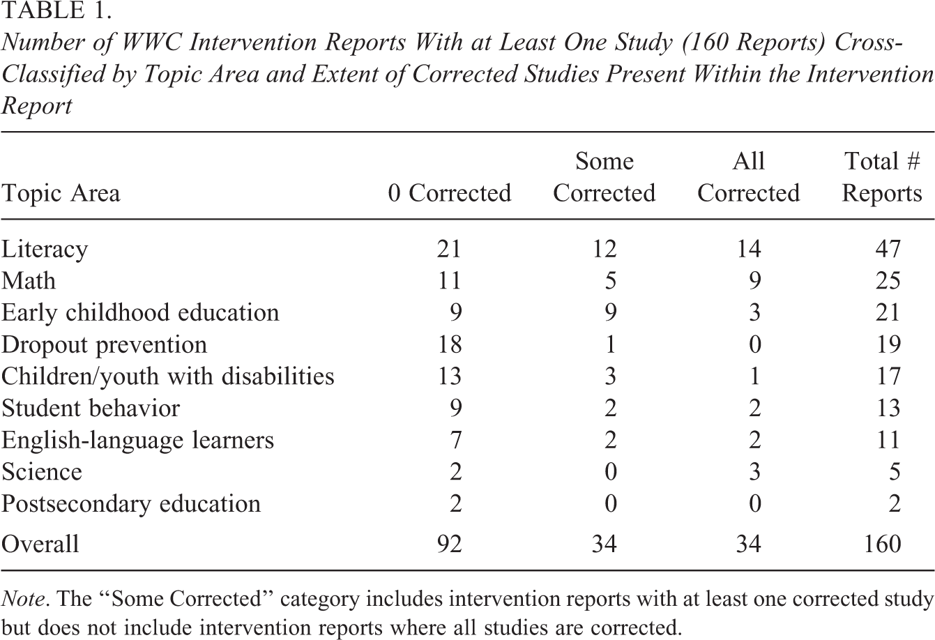
Note. The “Some Corrected” category includes intervention reports with at least one corrected study but does not include intervention reports where all studies are corrected.
This article will extend the Hedges correction to a more general class of models in order to (a) characterize the performance of the Hedges correction when it is applied to situations with additional fixed effects and (b) explore the limits of correcting significance tests with the generalized correction strategy. This article is organized as follows: The next section introduces the general mixed effects model, which we will use to extend the Hedges correction. The second section presents several new results: a derivation of a generalized Hedges correction, its distributional properties, and a limited-information test statistic based on achievable bounds of the correction that can be used in practical situations. The third section explores the relationships between the Hedges, WWC, and generalized corrections, and the fourth section considers the power implications of correcting significance tests. The fifth section outlines the implication of these new results for education policy and the sixth section closes with a discussion.
A Mixed Effects Model and the Hedges Correction
Consider the following the normal mixed effects model:

where
Consider this model for the case where there are two treatment conditions i = 1, 2 and Ji
schools per treatment condition. Let the number of students in school (i, j) be denoted as Kij
and let

where

where

where

where the random effect of school membership has induced a correlation in the error term
We simplify the notation by aggregating the (i, j) groups together:
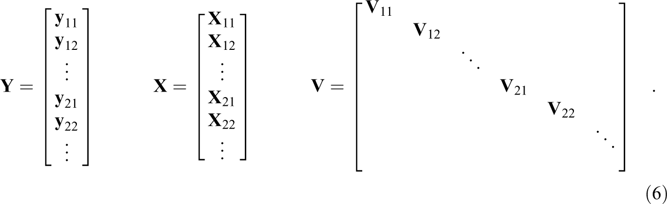
This allows us to express Equation 2, or any other mixed model with homogeneous variance, as:

without explicitly tracking the (i, j) block structure.
The model studied by Hedges (2007) is a special case of the model in Equation 7 where (a) the only fixed effect included in the model is the fixed effect of treatment and (b) the ICC of school membership is assumed known. When the value of the ICC is known, the optimal approach for parameter estimation and hypothesis testing is generalized least squares (GLS; Graybill, 1976). In the special case when the ICC is known to be zero, the ordinary least squares (OLS) estimates and tests are identical to their GLS counterparts. In the general case, however, where the ICC is not zero, OLS estimates have higher mean squared errors and OLS test statistics are anticonservative.
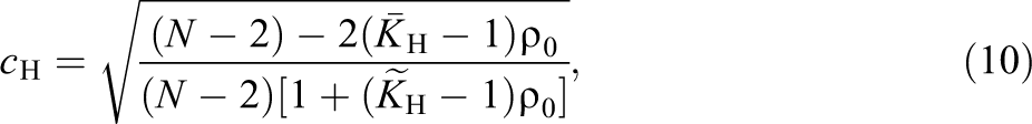
Hedges (2007) considered the consequences of calculating a t-test for the hypothesis of no treatment effect using OLS when the ICC is nonzero, that is, an independent two-sample t-test. For this case, Hedges derived the distribution of the OLS t-test when the data were generated with a given, known ICC denoted by ρ0. He then used that distribution to derive a constant factor such that the constant factor times the OLS t-statistic is approximately t distributed. In the case of balanced data, where N is the total number of observations and K is the number of students in every school, the correction is given by:
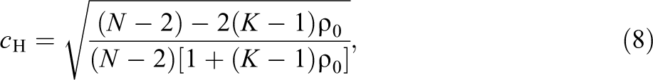
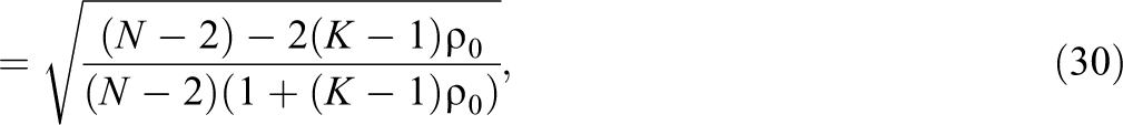
such that if we denote t OLS as the OLS t-test, then c H⋅t OLS is approximately t distributed with:

degrees of freedom. Note that h can be much less than the N − 2 degrees of freedom that would normally be assumed. For example, when N ≫ (Kρ0)2, h is approximately
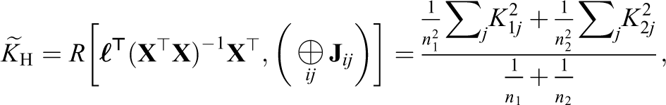
In the case of unbalanced data, the Hedges correction has a similar form. Let Kij be the number of students in school (i, j), as in Equation 2. Let the number of students in treatment condition i be ni = ∑ j Kij and define two measures of a typical school size as:
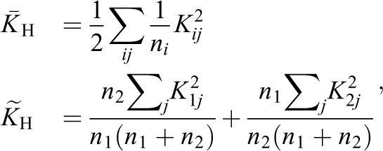
such that both
such that c H ⋅ t OLS is approximately t distributed with often far fewer than N − 2 degrees of freedom (Hedges, 2007, equation 16, p. 166).
The Hedges correction, however, is somewhat impractical to use for unbalanced data because it requires that the size of every group be known, and a complete enumeration of group sizes is rarely present in study reports. Due to this complexity, the WWC uses a simplified version of c
H where
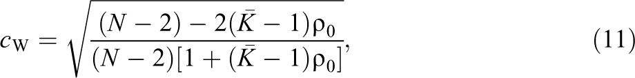
such that a corrected t-test is simply c
W ⋅ t
OLS. The WWC assumes this corrected test has the same degrees of freedom as in the balanced case of Equation 9 except that K is replaced with
To illustrate the potential consequences of this type of misspecification in the context of a group randomized experiment, we present an educational intervention that was analyzed incorrectly by the original authors and corrected by the WWC. In this case, the simplified Hedges correction used by the WWC is a poor approximation to a reanalysis of the data for two reasons: First, the WWC chose the ICC two times larger than the ICC that would have been estimated from original data, and second, the originally reported test statistic accounted for fixed teacher effects and the Hedges correction does not account for fixed effects beyond that of treatment.
The specific experiment we consider was conducted by Carnegie Learning, Inc. in Moore, Oklahoma, to study the effectiveness of their Cognitive Tutor Algebra I curriculum during the 2000–2001 school year. For this motivating example, we focus on the main academic outcome measured in the study, the end of year student scores on the Educational Testing Service (ETS) Algebra I exam. The study included 255 students taught in 16 classrooms by six teachers in three schools. Further details on the experiment can be found in the initial report by Morgan and Ritter (2002). We thank Steve Ritter of Carnegie Learning, Inc. for providing us with a copy of the original data.
Notably, the experiment used a within-teacher design. Each class period that a participating teacher taught was randomly assigned to either a Cognitive Tutor condition or a control condition. Once the teacher-to-period assignments were made, the schools used their “standard procedures” to enroll students in periods where Algebra was offered. Empirically, this kind of registrar-based assignment is equivalent to group randomized assignment, as the students who are assigned to the same class period by the registrar may share characteristics (Slavin, 2008). This clustering of students within classrooms may lead to correlated outcomes which will violate the assumptions of commonly used analysis of variance and analysis of covariance models. A class of models that accounts for clustering of students within classrooms are mixed effects models, specifically the two-level hierarchical model with a nonzero ICC for the effect of classroom membership in Equation 2.
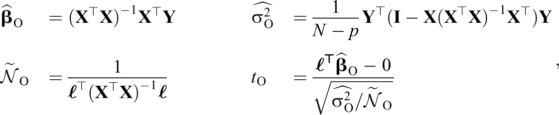
We consider two different approaches to analyzing the Moore experiment: Approach A, a marginal analysis that considers only treatment assignment and ignores the within-teacher nature of the experimental design; and Approach B, a within-teacher analysis that models teacher effects as fixed. Within each approach, we consider two ways to calculate a test statistic for the hypothesis of no treatment difference: Case 1, a test statistic based on the (mistaken) assumption that the ICC (ρ) is zero; and Case 2, a test statistic that accounts for the nonzero ICC estimated from the data using a two-level hierarchical model
Table 2 displays the results of Cases 1 and 2 as columns and Approaches A and B as rows. As expected, the misspecified t-statistics in the Case 1 column are much larger than the REML t-statistics in the Case 2 column. This anticonservative effect of model misspecification is most noticeable for the Approach B t-statistics in the second row. The misspecified Case 1B test statistic is significant at the .01 level, while the REML Case 2B t-statistic is only significant at the .10 level.
The t-Statistics Test No Treatment Difference and Are Coded Graphically for Significance Based on a Two-Sided Test
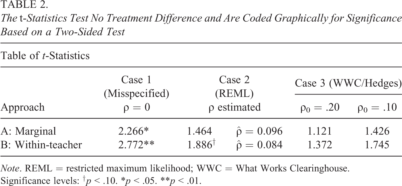
Note. REML = restricted maximum likelihood; WWC = What Works Clearinghouse.
Significance levels: † p < .10. *p < .05. **p < .01.
Table 2 also displays the results of the WWC’s simplified Hedges correction c W applied to the Case 1 t-statistic as Case 3 (WWC/Hedges). We report two versions of the correction to illustrate the two reasons why the WWC/Hedges correction broke down for this example: the first, where we calculate the correction with ρ0 = .20, as the WWC did due to the ETS exam being an academic outcome; and the second, where we assume the ICC is near the estimated value of ρ0 = .10 to isolate the differences between Approaches A and B. Note that the ρ0 = .20 column demonstrates the sensitivity of the correction to the accuracy of the ICC; the corrected tests are very conservative relative to the REML test statistics if the ICC assumed by the WWC is twice as large as the estimated ICC.
If the ICC is correctly specified, however, for Case 3A, the WWC/Hedges correction is able to scale the misspecified t-statistic from Case 1A to match the REML t-statistic from Case 2A. This may be expected because Approach A represents the situation for which the WWC/Hedges correction was derived, and the assumed ICC is close to the estimated ICC. For Case 3B, however, the WWC/Hedges corrected t-statistic does not match the REML t-statistic from Case 2B, even though the assumed ICC is close to the estimated ICC. Further note that, in this example, the test statistics are also of differing significance levels, with the corrected test statistic of Case 3B not achieving statistical significance at the .10 level. These differences between the Case 2B and Case 3B test statistics are not surprising, given that the anticonservative effect of model misspecification is mediated by the presence or absence of fixed teacher effects in this example, and neither the Hedges correction nor its simplified WWC variant was derived to account for such additional fixed effects.
The results of Hedges (2007) demonstrate that without access to the original data, a misspecified test statistic can be scaled to approximate the distribution of the correct statistical test, for example, the corrected Case 3A test statistic matches that of the REML Case 2A test statistic when the ICC is known. The Hedges correction, however, was derived for a very specific model, the special case of the model in Equation 7 where the only fixed effect included in the model is the fixed effect of treatment. In the next section, we will consider a generalization of the Hedges correction to the full model, in order that more complex analyses, such as the within-teacher model of Approach B, can also be corrected.
A Generalization of the Hedges Correction
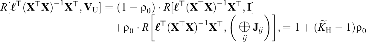
As first discussed by Hedges (2007), an approach for dealing with model misspecification in the context of meta-analysis is to develop a scaling factor such that the misspecified t-statistic is scaled to control its Type I error. For our extension of the Hedges correction, we consider two practical features of a scaling factor approach: (a) that the distribution of the corrected t-statistic approximates the distribution of the t-statistic that would have been used if the model were not misspecified and (b) that the calculation of the correction would not require access to individual-level data,
Formally, we assume that a given experiment was conducted such that the data could reasonably be modeled as being produced by a data generating model
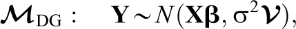
where

where
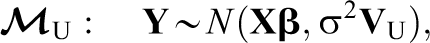
where
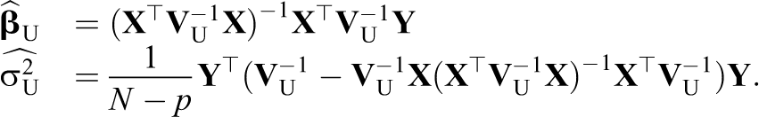
We consider correcting hypothesis tests that can be expressed as a linear combination of the fixed effects being equal to zero.

with either one-sided or two-sided alternatives and restrict our attention to studying the differences between the OLS and GLS estimators and test statistics when
Under
A commonly used test for the hypothesis in Equation 12 under

where

Under
then the distribution of t
U under

where

We note that as the effective sample size
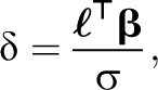
The originally reported model
so that under

where
Under
First, we note that, under
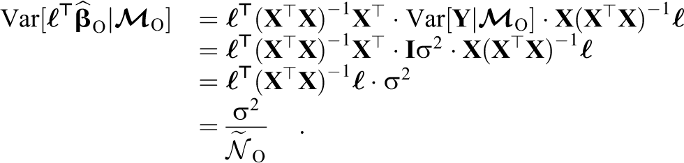
If we choose to replace σ2 with its UMVUE under

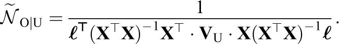
Second, we construct a Wald-like test for
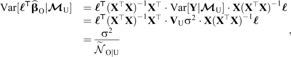
where we have defined the effective sample size of
Since

as the bias-corrected variance estimator. Theorem 3 in Appendix A, available in the online version of the journal, gives that

We express W O|U in terms of t O by multiplying the numerator and denominator of W O|U by the denominator of t O so that:
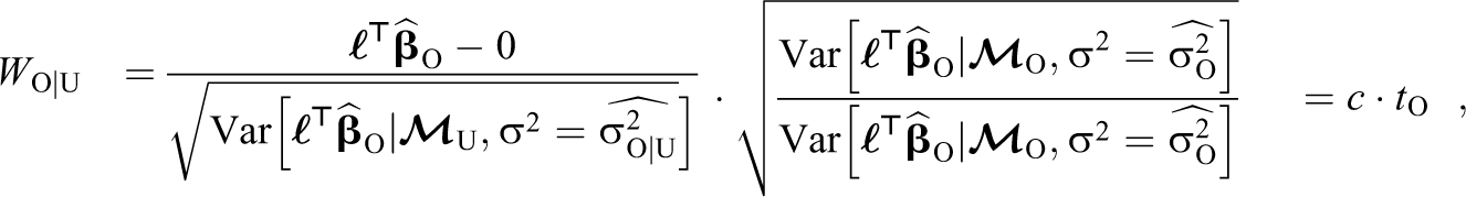
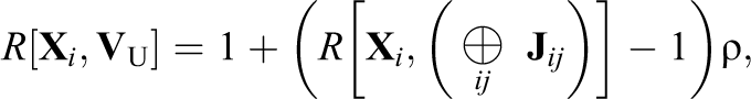
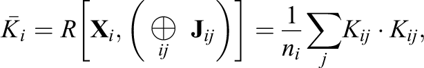
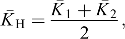
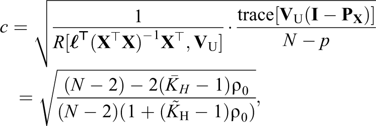
where we have defined
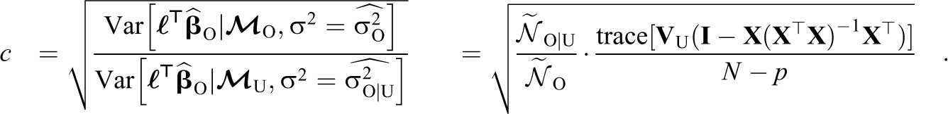
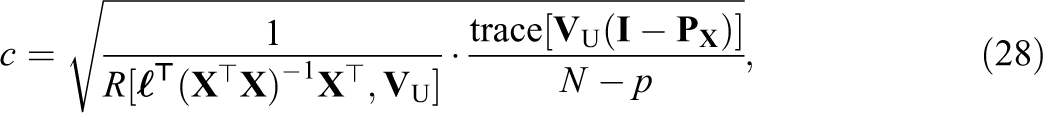
We can simplify the form of c by defining
so that

and c can be expressed as:
One interpretation of c is as a scaling factor to update the Wald test under

We note that under
One possible small sample approximation of the distribution of c ⋅ t O is:

which is a Satterthwaite approximation, where the derivation of the degrees of freedom h follows directly from the cumulants of
The results of Equations 18 and 19, however, cannot be used in practical situations by a meta-analyst. For these results to be used, either
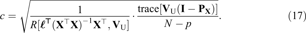
We propose a feasible correction based on a lower bound of c that is (a) equal to c in special cases and (b) can feasibly be calculated by a meta-analyst. These new results rely on a second interpretation of c; specifically, that it is the square root of the bias under
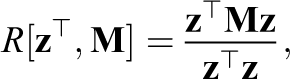
Under this second interpretation, c is well studied. For example, Swindel (1968) gives achievable bounds on c that depend on the eigenvalues of

Following Swindel (1968), we factor and bound c from Equation 17 into two terms. First, Swindel quotes the min–max theorem (Rao, 1973) to bound the Rayleigh quotient by the largest and smallest eigenvalues of

Second, Swindel proves that the term arising from the bias of
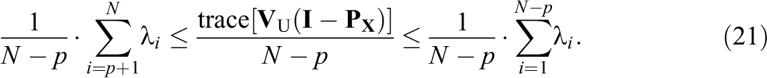
Using the identity
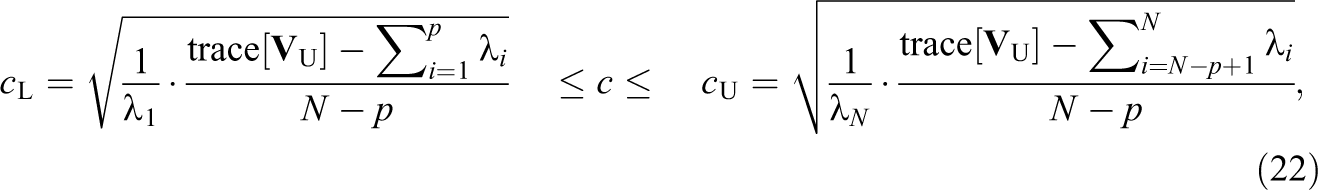
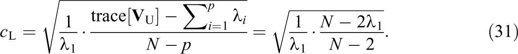
where N and p are the dimensions of

which can be used to judge whether or not the large sample normal approximation applies.
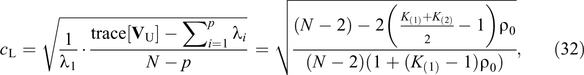
The lower bound of the corrected test is then:

We note that c
L ⋅ t
O is calculated without access to the value of
We refer to c ⋅ t O as the full-information corrected test statistic and c L ⋅ t O as the limited-information corrected test statistic. The limited-information corrected test has the property of always controlling its Type I error relative to c ⋅ t O for hypothesis tests performed with the rejection region of c ⋅ t O. To see this, note that under the null hypothesis, Equation 18 implies that:
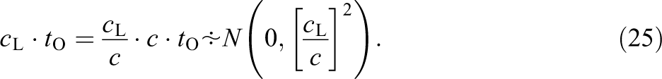
Since Equation 22 implies that c L/c ≤ 1, the mass of the distribution of c L ⋅ t O is more concentrated around zero than c ⋅ t O. The tail area of the rejection region, therefore, is always less than that of c ⋅ t O, that is, c L ⋅ t O has a Type I error less than or equal to c ⋅ t O.
Given these two interpretations of c, the generalization of the Hedges correction to mixed effects models has two parts: (a) a full-information correction given in Equation 17, which can be used in situations where either
Relationships Between the WWC, Hedges, and Generalized Corrections
To examine the relationships between the various corrections, we partition the model of Equation 7 into four cases of relevance to estimating treatment effects in group randomized studies. Case I considers a model with only treatment fixed effects and balanced group sizes, Case II a model with treatment fixed effects and unbalanced group sizes, Case III a model with an additional fixed effect and unbalanced group sizes, and Case IV a model with multiple additional fixed effects and unbalanced group sizes.
In Case I, all four corrections, the WWC, Hedges, generalized, and limited-information corrections, are equal to Equation 8. They are, consequently, feasible to calculate, as N and K are likely to be given in the original report and ρ0 is assumed to be known. Furthermore, we show that the corrected test controls its Type I error.
In Case II, the Hedges and generalized corrections are equal to Equation 10 while the WWC and limited information each have their own forms. The Hedges and generalized corrections cannot be calculated because they require knowledge of every group size, which is unlikely to be given in the original report. Although the WWC and limited-information corrections are feasible to calculate in this case, we show that the WWC correction fails to control the Type I error of the corrected test, while the limited-information corrected test controls its Type I error.
In Cases III and IV, which are the most common cases encountered in practical settings, the form of each correction is unique. We show that only the generalized and limited-information corrected tests control their Type I errors. We also show that the generalized correction is infeasible to calculate because it relies on knowing the degree to which randomization did or did not balance covariates between groups. Additionally, the limited-information correction can be difficult to calculate because it requires knowledge of the size of the p largest groups, which is three for Case III and can much larger for Case IV. For these situations, we suggest a modified form of the limited-information correction that always controls its Type I error, only requires knowledge of the size of the largest group, and in large samples is equal to c L.
To derive these results, we consider design matrices that are extensions of the design matrix studied by Hedges (2007) to derive c H in Equation 10:

where

where
Note that the regularity conditions from the convergence result of Equation 18 are met. Conditions 1 and 2 follow directly. To show Condition 3, that the ratio of eigenvalues is bounded, we give the ordered eigenvalues of
In all cases, we consider the null hypothesis of interest as that of a zero treatment effect, that is,
Case I: Treatment Fixed Effects and Balanced Groups
Case I was studied by Hedges (2007) to derive the balanced Hedges correction of Equation 8. When the data are balanced,
This balance gives the matrices
Under these conditions, all four corrections are equal. First, we show that c = c H. Note the Rayleigh quotient term of c is equal to λ1:

Further note that (a)

Therefore, the full-information correction can be expressed as:

which is equal to the Hedges correction of Equation 8: Second, c is equivalent to the WWC correction of Equation 11, because
For Case I, therefore, all four corrections are equal: c = c H = c L = c W. Furthermore, all the corrections can be calculated in practice by a meta-analyst: (a) it is likely that K and N are given in the original research report and (b) the value of ρ0 is assumed to be known a priori.
Case II: Treatment Fixed Effects and Unbalanced Groups
Case II was studied by Hedges (2007) to derive the Hedges correction of Equation 10. The design matrix is
For Case II, the full-information correction c is equal to the Hedges correction of Equation 10. The Rayleigh quotient term of c can be expressed in a functional form that is similar to an eigenvalue of
where we have defined:
as the effective group size, which is itself a Rayleigh quotient. Note that we chose the notation
The trace term of c can be expressed in terms of Rayleigh quotients by noting that (a) the projection matrix can be split into two rank one projections and (b) the cyclic permutation property of the trace operator allows the rank one projections to be permuted into Rayleigh quotients. Specifically, if we define
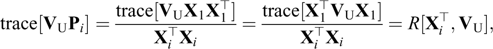
such that

We can express this in the form given by Hedges by noting that:
and defining
where
which is identical to the

The full-information correction is then
which is equal to the Hedges correction from Equation 10.
The limited-information correction differs from the full-information and Hedges corrections:
because it depends only on the largest and second largest group sizes. In general, c will differ from c
L because
The WWC correction of Equation 11 also differs from the other corrections for much the same reason: The simple average
The relationships between the K values imply that c
L should be preferred over c
W. Since

so that
For Case II, therefore, the corrections differ. If all of the group sizes have been reported in the original report, c = c H can be calculated. If the largest two group sizes are available (or reasonable values for them can be assumed), then c L can be calculated. The WWC correction, however, should be avoided, as it does not control its Type I error in all cases with unbalanced data.
Case III: An Additional Fixed Effect and Unbalanced Group Sizes
The Case III model considers a more general group randomized experiment than Case II in that a covariate has been included in the design matrix. Specifically,

where

is the pooled variance estimator of
For Case III, the relationship between c, c
H, c
L, and c
W depends on d
A and the variation in
where
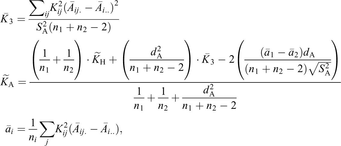
such that the cross terms
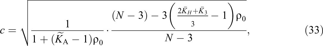
To facilitate comparisons between the various corrections, we consider their large sample forms. In large samples,

where large is defined as N being much larger than 3K (1)ρ0. The large sample forms of c W, c H, and c L are similar:

Although the large sample form of the Case III expression for c is simple, the expression for
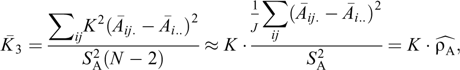
where we have approximated N − 2 ≈ N and defined:
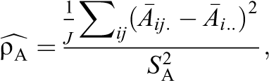
as an ICC-like quantity for the covariate
The form of
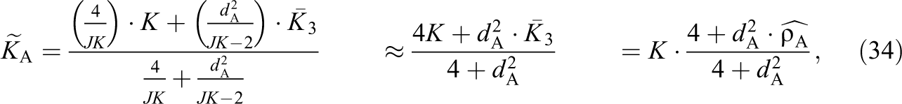
where we have approximated JK − 2 ≈ JK.
If the between-group variation in
In Case III, the WWC-corrected test will not control its Type I error relative to c ⋅ t
O for much the same reason as in Case II: There is no consistent relationship between
In Case III, therefore, neither the WWC-corrected test nor the Hedges-corrected test will control their Type I errors, only the full-information and limited-information corrected tests will control their Type I errors. Furthermore, the full-information correction is unlikely to be able to be calculated because it is likely that neither the group sizes necessary to calculate
Case IV: Additional Fixed Effects
The Case IV model considers a more general group randomized experiment than Case III in that additional covariates can be included in the design matrix. Specifically,

where
Although the extension of Case III to Case IV is conceptually straightforward, it is notationally burdensome and the outcome is the same as Case III. Namely, that c ⋅ t O and c L ⋅ t O are the only corrected tests to control their Type I error and that, of these, only c L ⋅ t O has a reasonable chance of being feasible to calculate.
Note that if the number of covariates included in the model is too large, then c
L may be difficult to calculate directly because the size of the p largest groups may not have been given in the original report. In this case, we suggest a lower bound of c
L, which we define by replacing every eigenvalue of

Note that since
For Case IV, therefore, we recommend c
L ⋅ t
O if the p largest group sizes are available and
The Power of Corrected Tests
In this section, we show that the power of corrected tests, however, is necessarily low. There are two reasons for this: First, the power of a reanalysis of the data is necessarily lower than that of the original study, and second, for practical situations, controlling the Type I error of the corrected test requires the test to be more conservative than a reanalysis, implying the power is less than that of a reanalysis. We will show, for example, that in the context of education research, the power of a corrected test is often less than one third and can approach zero in some cases.
To simplify our discussion, we assume that the original authors planned the study for a one-sided test, and the resulting sample sizes are sufficiently large enough that all the test statistics we consider are approximately normally distributed. Specifically, we assume the original analysts planned their study to detect a minimally detectable effect size (MDES), say MDESO, at a Type I error of α and a power of 1 − β. Let Φ[] be the cumulative distribution function of a standard normal, and let z α and z β be critical values such that Φ[−zα ] = α and Φ[−z β] = β. The original authors would have chosen samples sizes and covariates such that,

because Equation 15 implies that for this choice of

The power of a reanalysis of the data, that is, the power of t
U under

so that for the same Type I error and MDES, Equation 14 implies the power of t
U under

where the tightness of the bound depends on the tightness of Equation 35, that is, whether or not the study was overpowered to detect MDESO. Note that if the original study was planned to be exactly powered to detect MDESO, then as K grows, the power of the test approaches
To put this in context, we consider how low the power can be for a study modeled after the Cognitive Tutor study. If we assume the experiment was planned under
The performance of a corrected test is necessarily worse than this. Recall that, in practical situations, the only corrected test that both controls its Type I error and is feasible to calculate by a meta-analyst is c
L ⋅ t
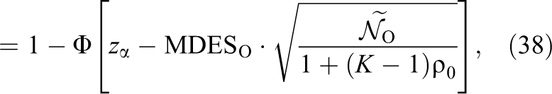
O. We show in Appendix C, available in the online version of the journal, that the large sample power of c
L ⋅ t
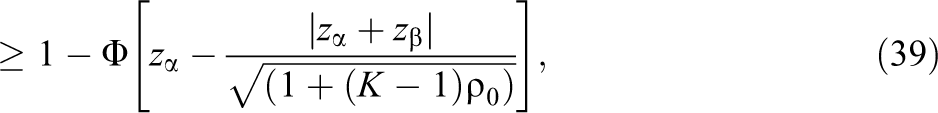
O with a one-sided alternative under

where

Note that the upper bound on the power of the corrected test is the power of reanalysis of the data, for example, in the special case of a study designed to exactly achieve a power of 1 − β such that if the group sizes were balanced, then πU is equal to Equation 39.
To put these bounds in context, we continue the Cognitive Tutor example. Morgan and Ritter (2002) reports the size of the largest group as 26 students. Under the same assumptions as before, the formulas for πL and πU imply that the power of c
L ⋅ t
O under
Figure 1 extends the Cognitive Tutor example by comparing the nominal power of t
O under

Comparison of upper (π
U) and lower (π
L) bounds on the power of cL
⋅ tO
under
Figure 1 implies that for group sizes and ICC values that are common in education research, the power of a corrected test is often less than one third and can approach zero in some cases. For example, if the ICC is 0.20, the power of c L ⋅ t O will be less than one third if the size of the largest group is greater than 18 students. The power can even approach zero: The lower bound of the power of c L ⋅ t O quickly approaches zero, implying that, in some cases, the power of c L ⋅ t O will also approach zero because the bound is tight. If the ICC is 0.10, the power of c L ⋅ t O improves, but the main message is the same: The power of a corrected test is low and can approach zero in some cases.
Implications for Education Policy
This research implies that the statistical methods the WWC uses for meta-analysis prevent it from finding effective interventions. In this section, we will show that adding any low power study, for example, either a corrected test statistic or a test statistic based on a reanalysis of the data, to an intervention report will lower the overall power of the intervention report relative to simply excluding the study. Since at least two out of five intervention reports contain corrected, that is, necessarily low power studies, the current WWC meta-analysis methods are inappropriate.
The WWC currently uses a variant of vote-counting meta-analysis to classify an intervention into one of the six categories, ranging from “positive effects” to “negative effects” (WWC, 2014, pp. 27–28, table IV.3). To simplify our discussion, we consider a vote-counting meta-analysis with only two categories: positive effects or not positive effects. Let there be m identical studies that were designed to detect a nonzero treatment effect with a power of π for a one-sided test. Each of the m studies are sorted into two bins according to the outcome of the significance test: a bin for tests that are statistically significant and a bin for tests that fail to reject the null hypothesis. The rejection rule for the vote-counting procedure is to reject the overall null hypothesis of no treatment effect if there are more of the m tests in the statistically significant bin than otherwise. Formally, if we let U be the number of studies in the statistically significant bin, then we reject the overall null hypothesis if U/m > 1/2.
Hedges and Olkin (1980) demonstrated that for such a vote-counting meta-analysis, the power of the meta-analysis can go to zero if the power of each of the m studies is less than the threshold given in the rejection rule. In this case, if π < 1/2, then the power of the meta-analysis decreases as m increases. Briefly, their argument is that U has a binomial distribution, so the central limit theorem gives the large sample distribution of U/m as:

This implies that as m increases, U/m will become concentrated around π. Since the vote-counting meta-analysis rejects the null when U/m > 1/2, the power goes to zero in the case where π < 1/2.
Although the vote-counting procedure used by the WWC is more complex than the simple example given here, it shares a common property: If the power of a test statistic is less than the threshold used to reject the null hypothesis, then including this test statistic in the meta-analysis will lower the power of the meta-analysis. The WWC threshold is one third: Their recommendation of an intervention depends on whether or not the majority of studies included in the meta-analysis found a statistically significant and positive effect, statistically significant and negative effect, or did not achieve statistical significance. Since the power of both corrected and reanalyzed significance tests is commonly less than one third, including either in an intervention report will lower the power of the intervention report relative to simply excluding that study. We recommend, therefore, that the WWC change from vote-counting meta-analysis to a method that is able to synthesize the results of low power studies such as fixed effects meta-analysis.
Discussion
The aim of the evidence-based education movement is twofold: (a) to determine the best practices from scientifically rigorous studies and (b) to apply those best practices to educational decision-making (Shavelson & Towne, 2002). Throughout its history, however, the evidence-based education movement has struggled with the low quality of education research (Lagemann, 2000). For example, a common error is that an experiment will be designed to randomize entire schools to treatment and control conditions but then is analyzed ignoring the grouped nature of the randomization (Song & Herman, 2010). This error is well known to lead to invalid conclusions because it overstates the statistical significance of the treatment effect.
This error also leads to low power. If the original, incorrectly calculated test statistic is corrected, then the corrected test will control its Type I error, but as we have shown, it will necessarily have low power. The prevalence of incorrectly analyzed studies in education research, therefore, requires the WWC to use methods capable of combining the results of low power studies. Their current method cannot: adding any low power test (corrected or reanalyzed) to an intervention report will lower its overall power, that is, its ability to detect what works. The WWC, therefore, should cease attempting to correct significance tests and instead adopt a method of meta-analysis that, at a minimum, could effectively combine results from low power, for example, reanalyzed, studies.
More generally, the low power of a reanalysis makes it difficult to interpret the results of a corrected test statistic in the context of a single study. Since the power of a reanalysis is often approximately one third, at least two thirds of the time a corrected test will fail to reject the null even though the intervention has a positive effect. This implies that the majority of the time a corrected test statistic will fail to reject the null (95% if the null is true, at least 66% if the null is false) regardless of the effectiveness of the intervention. If the most likely outcome is a null result, what guidance about the effectiveness of an intervention can be given to policy makers, especially if a null result is observed?
Given these operating characteristics, it is difficult to recommend correcting significance tests for general use. Instead, we recommend simply discarding studies that would require correction until either a reanalysis using individual-level data and models that appropriately account for the design is available or new methods for the meta-analysis of incorrectly analyzed studies are developed. Given the prevalence of incorrectly analyzed studies, such methods are an important area for future research.
Footnotes
Declaration of Conflicting Interests
The author(s) declared no potential conflicts of interest with respect to the research, authorship, and/or publication of this article. The views and conclusions contained in this document are solely those of the individual creator(s) and should not be interpreted as representing official policies, either expressed or implied, of the Software Engineering Institute, Carnegie Mellon University, the U.S. Air Force, the U.S. Department of Defense, or the U.S. Government.
Funding
This work was supported in part by Institute of Education Sciences training grants to Carnegie Mellon University (#R305B090023) and Northwestern University (#R305B100027).
References
Supplementary Material
Please find the following supplemental material available below.
For Open Access articles published under a Creative Commons License, all supplemental material carries the same license as the article it is associated with.
For non-Open Access articles published, all supplemental material carries a non-exclusive license, and permission requests for re-use of supplemental material or any part of supplemental material shall be sent directly to the copyright owner as specified in the copyright notice associated with the article.