Just Another Gibbs Sampler (JAGS)

Abstract

A review of the software Just Another Gibbs Sampler (JAGS) is provided. We cover aspects related to history and development and the elements a user needs to know to get started with the program, including (a) definition of the data, (b) definition of the model, (c) compilation of the model, and (d) initialization of the model. An example using a latent class model with large-scale education data is provided to illustrate how easily JAGS can be implemented in R. We also cover details surrounding the many programs implementing JAGS. We conclude with a discussion of the newest features and upcoming developments. JAGS is constantly evolving and is developing into a flexible, user-friendly program with many benefits for Bayesian inference.

Keywords

Bayesian inference statistical computing JAGS just another Gibbs sampler

Just Another Gibbs Sampler (JAGS) was developed by Martyn Plummer as an open-source program for analysis and statistical inference of Bayesian hierarchical models. JAGS was first released in 2003, and at the time of writing this article, JAGS was in version 4.3.0. Since 2006, JAGS and its related materials have been downloaded over 200,000 times around the world. JAGS and other relevant resources (e.g., examples and manuals) can be downloaded from https://sourceforge.net/projects/mcmc-jags/files/.

Development of JAGS

JAGS was developed using the dialect of Bayesian inference Using Gibbs Sampling (BUGS) language, which uses the Markov chain Monte Carlo (MCMC) estimation algorithm for Bayesian inference. The BUGS project was initially designed in 1989, based on developments from artificial intelligence (Lunn, Spiegelhalter, Thomas, & Best, 2009). Conceptually, the BUGS language uses directed acyclic graphs (DAGs) as the basis for model specification. In short, DAGs capture relationships among objects by using declarative statements that allow for uncertainty to be represented with probability distributions. DAGs are subsequently converted into model code and run via the MCMC estimation algorithm through an inference engine.

WinBUGS (Lunn et al., 2009) became the first widely popular BUGS program to implement Bayesian estimation via MCMC methods. In 2004, the BUGS team released OpenBUGS (Thomas, O’Hara, Ligges, & Sturz, 2006), which has greater extensibility and flexibility than its predecessor. The last patch for WinBUGS was released in 2007, when the development team decided to focus exclusively on the OpenBUGS project.

JAGS was created to be compatible with the BUGS software but is arguably more extendible, flexible, and user-friendly than the BUGS software. Differences between WinBUGS, OpenBUGS, and JAGS are explained below in the section titled “JAGS Compared to Other Bayesian Software.”

What the User Needs to Know About JAGS

JAGS uses MCMC algorithms to sample from probability distributions. JAGS was initially developed to be a clone of WinBUGS and OpenBUGS, while allowing its users additional flexibility to directly modify the program. JAGS uses the BUGS language; however, unlike WinBUGS, it is able to run on platforms other than Windows (e.g., Unix, Linux, or OS X). Additionally, JAGS users are able to create their own modules to extend the program’s capabilities. A JAGS module is a general term that can encompass various functions, distributions, and samplers—the latter of which refers to specific sampling algorithms (e.g., the Gibbs sampler) used with the MCMC estimation algorithm. Several JAGS modules have been created for use with the R software (R Core Team, 2016). For instance, the ParetoPrior (Denwood, 2015b) and jags-wiener (e.g., Nunez, Srinivasan, & Vandekerckhove, 2015) stand-alone modules—as well as their corresponding R packages (i.e., runjags and RWiener; Denwood & Plummer, 2016; Wabersich, 2014)—allow for the inclusion of prior distributions and functions that are currently unavailable in base versions of JAGS, WinBUGS, or OpenBUGS (e.g., a half-Cauchy prior). For a detailed description of procedures used to create a JAGS module, see Wabersich and Vandekerckhove (2014).

JAGS does not have a built-in graphical user interface (GUI).¹ Instead, it can be run directly from the command line. However, since the base program uses C++ language, existing software written in C or Fortran (e.g., R, MATLAB, Python, or Stata) can be easily used in conjunction with JAGS. JAGS is most commonly called from the R programming environment, and it is designed to work closely with the R language (Plummer, 2013). We describe how JAGS interfaces with R in a subsequent section.

JAGS Implementation

In this section, we focus on important details related to model specification and the implementation process. The key elements for running JAGS include (a) definition of the data, (b) definition of the model, (c) compilation of the model, and (d) initialization of the model. To help solidify these concepts, we reference code, as it relates to an applied example of latent class analysis (LCA) throughout. LCA is a statistical model used to identify latent (or unobserved) groups of individuals based on patterns of responses to observed indicators (or items). The application of LCA is fully explained in a subsequent section, where we present an example using large-scale education data.

Definition of the Data

Users may define the data in several different ways depending on how JAGS is being used (e.g., calls from R can be more flexible than command line invocations). The data and the model are typically specified in different files, but JAGS allows users to flexibly incorporate them simultaneously. For instance, the same script can be used to define the data and model in adjacent blocks, using functions that call data being generated in the same model for concomitant use (e.g., with the “cut” function), or by passing data created from a previous model run to a subsequent run; the latter of which is particularly useful when conducting simulation studies. Data may also be defined using calls to a function, with a character string, or by placing it in a separate text file using the format created by the dump() function in R. Data can also be defined as objects in R that are passed to the model, or within the model block itself (e.g., to specify constants for stochastic nodes). In the applied example presented below, we specify the data file by defining an object in R (e.g., lca <- read.table(“…/PISA_data.txt”, header = TRUE)).

Definition of the Model

The model is defined using variations of the BUGS language. Models can be called with script files, text files, model strings, or through function calls. In a later section, we demonstrate an applied example, where the model is specified within R and saved as a text file. The model file is initiated by calling the model{} function. Despite JAGS’ growing functionality, there are certain rules that must be followed when defining a model. Relationships between local model components are structured using nodes (represented as vectors in the form of different types of arrays). The graphical format describes the model through various node definitions. Models formatted in this manner consist of child nodes (i.e., the innermost part of the graph), parent nodes (i.e., the directed edges of the graph), and constant nodes (i.e., the outermost part of the graph). The keyword model is used to signify the beginning of a model block, followed by a series of nodal relationships embedded within curly brackets {}. A stochastic node represents a random variable in the model. Stochastic nodes are represented with one or more names depending on the choice of variable definitions, and blocks can be specified for sets of stochastic nodes using for loops in the model. These nodes are followed by a tilde (∼) symbol, a distribution name, and subsequently followed by comma-separated parameters (e.g., in our LCA example described below, we specified the following: for (k in 1:2) {pi[j, k] ∼ dbeta(.5,.5)}, where the code is explained in relation to the example below). A deterministic node is a value defined by a parent node. Deterministic nodes are represented by the child node’s name, followed by a left facing arrow (<-), and logical statement made up of parent nodes (e.g., class2[i] <- class[i]+1, as demonstrated in the applied example below).

Unfortunately, the use of JAGS’ model notation in conjunction with the array-style definitions for data can make it cumbersome and challenging to correctly specify certain types of models. In most instances, specifying for loops within each model block is necessary for defining the DAGs used by JAGS. Models with a hierarchical or multivariate structure can be particularly difficult to conceptualize as DAGs, and the way in which data are defined in JAGS often precludes the use of simple model definitions (e.g., use of matrix algebra is often prohibited).

Model definitions in JAGS must adhere to a certain set of restrictions imposed by the BUGS language. Reliance on the BUGS language can therefore be a major barrier when developing complex models. However, a plethora of accessible modeling examples (see, e.g., Kruschke, 2015) and Internet resources are available to JAGS users, which can serve as a foundation for model building. At the same time, JAGS is becoming quite user-friendly by allowing for the use of R-style formatting inside model code. Likewise, a major benefit of JAGS is the ability to omit data from the model, allowing for independent sampling from the prior distributions. Direct sampling from the prior distributions is a useful tool for ensuring that priors are being specified as intended. The data and model can often be set up relative to a user’s preferences. We therefore refer the reader to the JAGS User’s Guide (Plummer, 2015c) for specific details about the data and model setup.

Compilation of the Model

The model compilation process involves the conversion of model syntax into a graphical representation of the model in the format of a DAG, which is stored in the computer’s memory. At this stage, JAGS checks the model syntax for errors. If the model syntax is appropriately specified, then JAGS may subsequently require an adaptation phase, during which time the software decides upon the most appropriate samplers for each parameter. The length of the adaptation phase (i.e., the number of iterations specified before burn-in) can be manually requested by the user and may require longer periods depending on model complexity or unusual specifications (e.g., latent variable models can often be specified using data stacked in long format with indexical indicators pointing to different “groups” of variables or units, in wide format using multidimensional arrays, or a combination of both).

Initialization of the Model

In order to initialize a model, the user may specify starting values for the model parameters, along with a random number generator (RNG) and samplers for each parameter. Users can choose the initial values and which parameters to supply initial values for. For instance, the following illustrates how starting values can be set for parameters p and pi by defining initial values in an R object:

jags.inits <- function () {list(p=.3,

pi = structure(.Data=c(.7,.4,.7,.4,.7,.4,.7,

.4,.7,.4,.7,.4,.7,.4,.7,.4), Dim=c(8,2)))}

Parameters often do not require that the user specify initial values. For simple models (e.g., a basic regression model), for example, the specific choice of initial values may not have an impact on the posterior inference. Conversely, more complex models consisting of many unobserved (i.e., latent) variables often benefit from the careful selection of initial values (e.g., structural equation models). When initial values are not supplied for a given parameter, JAGS generates them by sampling from the specified prior distribution. Supplying appropriate initial values can improve chain mixing, reduce computation time, and aid model convergence. For complex models (e.g., multilevel finite mixture models [FMMs]), the burn-in period can be shortened and chain mixing can improve by running the model twice, where estimates from the first run are used to inform initial values for model parameters in the second run (see, e.g., Almond, 2014).

The recent major update in JAGS has made it possible to ensure that results from an analysis are completely reproducible. In particular, specifying the same pseudo-RNG name and RNG seed (i.e., a specific number) for each chain in an analysis will result in identical findings upon replication. Note, however, that without specifying an RNG name and corresponding seed explicitly, JAGS will set an RNG name from the base module at random and select a seed using the current timestamp. Thus, the RNG name and seed are important if users are concerned with reproducibility. Accounting for the RNG state can also be useful; for instance, to extend a user-specified model when convergence has not been obtained.²

Another aspect of JAGS that has undergone recent updates concerns a larger selection of samplers and modules than were previously available. In brief, different types of samplers are associated with different JAGS modules. The base module includes a variety of useful arithmetic operators that are synonymous with those used in R. With the base module, four RNG names are available, each of which can be used to specify a different RNG name for each chain in a given analysis. The BUGS module is loaded in JAGS by default and includes a long list of distributions and functions that can be called by the user. Modules that can be loaded manually include (a) the generalized linear model (GLM; which is recommended for most analyses and can improve performance for even very simple GLMs such as a basic logistic regression), (b) the mix module (for identifying finite mixtures of normal distributions), and (c) the multistate model module or merge module (which incorporates the matrix exponential function and the multistate distribution). Each of these modules allows users to call various functions and samplers that serve to enhance the extensibility of JAGS and maximize modeling efficiency. However, it is important to note that one should become familiar with the samplers associated with these modules before making manual adjustments. For instance, turning off the tempered transitions sampler in the mix module can result in considerable speed improvements, but between-chain label switching (defined in the next section) must be monitored closely under these conditions (Almond, 2014). Finally, the deviance information criterion (DIC) module has several monitors that can be useful for evaluating model fit. The DIC module calculates the deviance of the model (i.e., −2× the log likelihood), which can be used to compute a variety of model fit measures; for example, the pD, which is used as an indicator of the effective number of free parameters, and the Popt fit measure, which is used to compute the penalized expected deviance.

Like other Bayesian software programs that rely on MCMC for estimation, JAGS models can be slow to converge to a target distribution, particularly in the presence of models with highly correlated parameters, models that are weakly identified, or models that are highly complex. The implementation of alternative or redundant parameterizations and the use of hyperpriors can be used to overcome some of these potential limitations (see, e.g., Almond, 2014; Gelman & Hill, 2007; Ghosh & Dunson, 2009; Kruschke, 2015). Additionally, computation time and chain mixing can often be improved by manually selecting modules associated with the most appropriate samplers for specific sets of model parameters. Users should check regularly for version updates, as JAGS continually adds new samplers and builds upon the samplers that are readily available. The variety of samplers currently available in JAGS can be considered a key benefit of the program, especially when complex models are under investigation. Specifying multiple chains and allocating them to different computer cores or creating computer clusters can also reduce computation time. In such cases, it is common practice for users to specify disparate initial values for each chain as evidence that each chain is independently converging upon the same target distribution during the post-burn-in period.

Once the model has been initialized, users can manually set monitors on specific model parameters to record the simulated values (e.g., a trace monitor saves the sampled values for each iteration in a given chain). The monitored values are stored in the form of coda files. The coda package (Plummer, Best, Cowles, & Vines, 2006) in R is a popular tool for postprocessing coda files, allowing for the computation of summary statistics, convergence diagnostics, and plots.

An important consideration when saving samples for variables pertains to the amount of computer memory available. When files are run in R, the amount of computer memory can accumulate quickly depending on the number of monitored parameters. For complex models with a large number of variables, it is often useful to consider whether a monitor needs to be set for a given parameter.

An Example of LCA in JAGS Using a Large-Scale Database

In this section, we demonstrate an empirical application in JAGS utilizing the Program for International Student Association (PISA; Organization for Economic Co-operation and Development, 2014) database. PISA is an international survey administered triennially since 2000. Fifteen-year-old students from randomly selected schools worldwide are administered tests aimed at evaluating educational systems by assessing a student’s ability to apply knowledge obtained in school to real-life situations (e.g., balancing a checkbook). Tests include a mixture of open-ended and multiple-choice questions in key subjects: reading, mathematics, and science, with a focus on one subject in each year of assessment. For the purposes of this example, we use data from the 2012 PISA cycle, which evaluated students’ performance as well as their attitudes and self-reported aptitude in mathematics.

Approximately 510,000 students from 65 participating countries and economies completed the assessment in 2012. Here we concentrate only on data from the U.S. sample. This includes over 6,000 randomly selected students from 161 randomly selected schools. Because this example is intended solely for pedagogical purposes, we ignore the nesting of students within schools as well as cases with missing data. Eight mathematic self-efficacy items are used in this analysis (N = 3,196, after removing all cases with missing data). These items asked students to indicate their confidence level in performing a variety of mathematical tasks such as “Using a train timetable” or “Solving an equation: 3x + 5 = 17.” Student scores for these items were modified to represent whether students had confidence in their ability to solve the item (coded as 1) or did not have confidence (coded as 0). This coding scheme was used to highlight the ability for JAGS to handle dichotomous outcome variables. In this example, we demonstrate the implementation of an LCA with two latent subgroups and dichotomous outcome variables in JAGS. The model is displayed in Figure 1, with a categorical latent variable that defines the latent classes. There are eight observed indicators for the latent class variable, and conditional response probabilities are computed for each indicator. Typically, patterns of response probabilities will substantively differ across latent classes. 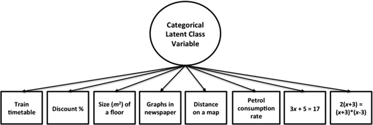We implemented analyses using the R2jags package (Su & Yajima, 2015) in R as a user interface with JAGS.

Figure 1.

Latent class model with eight categorical indicators.

To perform MCMC sampling of a posterior distribution in JAGS, we first define the prior, the likelihood, and the observed data. The user is not required to specify information about the posterior or the sampling mechanism used. Here, we allowed JAGS to determine the most appropriate sampler(s) to implement for each parameter. In JAGS, the likelihood and prior distribution are specified in the model statement. The basic model code is written in the BUGS language and read as follows (text following the # symbol is a note describing the preceding line of code):

sink(“C:/…/model.txt”) # Define where the text file will be stored

cat(“ # Begin character string for model

# Begin model definition

model{

# Data likelihood

for(i in 1: N){# Loop over observations (i.e., data rows)

class[i] ∼ dbern(p) # class proportions follow Bernoulli dist.

class2[i] <- class[i]+1 # Define placeholder for class membership

for(j in 1:8) {#Loop over items (i.e., data columns)

items[i, j] ∼ dbern(pi[j, class2[i]]) # Dichotomous items follow a Bernoulli distribution

} # End of j

} # End of i

# Prior distributions

p ∼ dunif(0,1) # Uniform prior

for (j in 1:8) {# Loop over items

for (k in 1:2) {# Loop over number of classes (k = 2)

pi[j, k] ∼ dbeta(.5,.5) # “U”-shaped beta (A.K.A. Jeffrey’s) prior

} # End of k

} # End of j

} # End of model

“, fill = TRUE) # End of character string

The first for loop says that latent class membership is modeled through a Bernoulli distribution with parameter value p. Here we define class proportions as p, using a uniform prior bounded at 0 and 1.³ The next for loop says that the item parameters are distributed Bernoulli, with parameter values pi. The final section of code shows that the values of pi come from a beta prior distribution with shape parameters .5 and .5, allowed to vary across latent classes (K = 2) and items (J = 8). We can fit this model in JAGS by first reading the PISA data into R and creating an object (lca). The code for this example is:

lca <- read.table(“…/PISA_data.txt”, header = TRUE)

jags.data <- list(N = 3196, items = structure

(.Data = lca))

#parameters to be monitored

jags.params <- c(“p”, “pi”)

#intial values

jags.inits <- function () {list(p=.3,

pi = structure(.Data=c(.7,.4,.7,.4,.7,.4,.7,

.4,.7,.4,.7,.4,.7,.4, .7,.4), Dim=c(8,2)))}

jagsfit <- jags(data = jags.data, inits = jags.intits,

param = jags.params, DIC = FALSE, n.chains = 1,

n.iter = 70000, n.thin = 1, n.burnin = 20000,

model.file = “…/model.txt”)

Once an object containing the PISA data is created, we define all of the observed variables within the model. Here we use N and items. Using the list()function to convert the data file into a JAGS format, we identify the number of observations (N = 3,196) and define the items by calling the R object lca. Next, we create an R object that identifies the unobserved parameters, class proportions (p), and item probabilities (pi). An R object was also created to hold initial values for each of the unobserved parameters. Lastly, within the jags function, we specify the data, model file, parameters to monitor, and initial values. The jags function automatically writes a JAGS script, calls the model, and saves the resulting simulations for later use. Although placed into R objects in this illustration, the data file location, monitored parameters, and initial values could have easily been written within the jags function.

A single Markov chain was used in the analysis. A total of 70,000 iterations were performed, with the first 20,000 iterations specified as burn-in. Markov chains for each variable were monitored for convergence, first by visual inspection using trace plots (available from the first author, along with full data set). Plots were examined for each parameter, including the class proportions and conditional item probabilities. Additionally, chains were monitored for convergence using the Gelman and Rubin (1992) convergence diagnostic.

The R output includes information regarding which iterations were used in the posterior estimation, the thinning interval (set at 1 for no thinning), and the number of chains used (a single chain was used to avoid between-chain label switching for the latent classes).⁴ The first 20,000 iterations were specified as burn-in, so each chain consisted of the last 50,000 iterations. Next, the posterior mean and standard deviation estimates for each parameter are produced. Each estimate represents the probability of answering confident to each question for each latent class. Looking at the pattern of responses across classes can provide an overall picture regarding the substantive meaning of the latent classes (Table 1 shows these patterns).

Table 1.

Latent Class Analysis Response Probabilities for 8 PISA Items

	Class 1	Class 2	Item Label
Item 1	0.939	0.594	Using a train timetable
Item 2	0.940	0.523	Calculating TV discount
Item 3	0.947	0.444	Calculating square meters of tiles
Item 4	0.971	0.671	Understanding graphs in newspapers
Item 5	0.821	0.182	Distance to scale
Item 6	0.918	0.379	Calculate petrol consumption rate
Item 7	0.993	0.873	Solving an equation: 3x + 5 = 17
Item 8	0.950	0.679	Solving an equation: 2(x + 3) = (x + 3)(x − 3)

Note. Values in the table represent conditional response probabilities. For example, Item 1 (Using a train timetable) has a 0.939 probability of endorsement, given membership in Class 1. PISA = Program for International Student Association.

Each row in Table 1 represents a different item in the questionnaire. The two columns of numbers are the probabilities of answering confident to the item, given that a person belongs to that latent class. That is, a person belonging to Class 1 has a 93.9% chance of saying that they were confident in “Using a train table.” By plotting these responses (see Figure 2), we can more easily ascertain the difference in response patterns across the two latent classes. The x-axis represents the item and the y-axis represents the probability of reporting being confident about completing a given item, given that one belongs to a particular latent class. Class 1 is comprised of individuals responding with confidence across all observed indicators, and Class 2 shows much more variability and lower confidence in certain items (e.g., Distance to scale). Overall, this example shows the relative ease to which models can be implemented in JAGS as well as the extreme overlap with the BUGS language.

Figure 2.

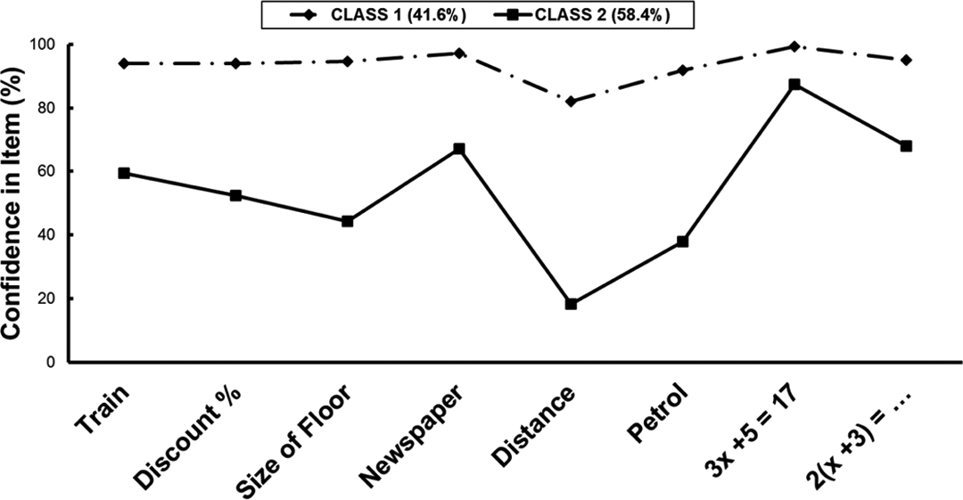
Latent class response probabilities. Notice that Class 1 shows high endorsement of confidence in all items and Class 2 is much more variable.

JAGS Interfacing With Other Software

We highlight some of the notable instances where other software programs or packages utilize JAGS—overtly or behind the scenes.

Interfacing With Packages in R

Rjags

The R programming environment has many packages that now implement JAGS for Bayesian inference. The package rjags was specifically created to implement the JAGS library within R (Plummer, Stukalov, & Denwood, 2016). The package first requires use of the BUGS language to define the model that is then read using the jags.model function. Once the model is updated then commands can be used to extract the samples, examine the posterior, and check convergence diagnostics through packages such as coda (Plummer, 2015a) or BOA (Smith, 2015). There are many examples and tutorials for implementing JAGS through this package available online, which makes this a great package for beginners interested in implementing JAGS (see, e.g., Jackman, 2009; Kruschke, 2015; White, 2010).

Runjags

The runjags (Denwood & Plummer, 2016) package contains additional features, making it ideal for more complex situations or data simulation studies. Specifically, this package offers the use of parallel processing for multiple chains and can be implemented in the context of a distributed computing cluster. There is automated control and monitoring of convergence diagnostics for chains within runjags. In addition, the run.jags.study function can be used to compare results from monitored variables to target values. This function makes runjags an ideal package for data simulation studies since model estimates can be directly compared to data generating values. The function extend.jags can be used to add an additional fixed number of samples to the original simulation. This feature can be particularly useful in situations where a chain abruptly deviates from convergence—the problematic portion of the chain can be removed and this function will add to the chain where sampling left off. The functions autorun.jags and autoextend.jags can be used to automatically extend the model until it reaches convergence according to the Gelman and Rubin (1992) diagnostic. Finally, there is an extension module that provides additional probability distributions that can be used as priors within the model. The added distributions include those from the Pareto family of distributions, the DuMouchel prior, and the half-Cauchy prior (Denwood & Plummer, 2016). A user guide for this package can be found in Denwood (2016).

R2jags

Another popular package in R that interfaces with JAGS is called R2jags (Su & Yajima, 2015). This package has a similar interface compared to R2WinBUGS (Sturtz, Ligges, & Gelman, 2015) and can be used to convert data from WinBUGS or OpenBUGS into JAGS format. Because of the similarities to BUGS, it is a popular choice for users already familiar with the BUGS programs. Similar to runjags, this package also has a built-in monitoring tool for assessing chain convergence and can handle parallel processing for multiple chains. R2jags also has the capability to allow a model to automatically run until convergence is reached based on a built-in assessment, which uses the Gelman and Rubin (1992) diagnostic.

R Packages Using JAGS Behind the Scenes

There has been a recent growth in other R packages implementing JAGS behind the scenes, where JAGS is used as the base for Bayesian inference within these packages. There are many packages using JAGS in this manner, and we provide a few examples here. First, the blavaan package (Merkle & Rosseel, 2016) uses runjags as a dependent for many of the Bayesian components. The blavaan package is used for Bayesian estimation of latent variable models (e.g., confirmatory factor analysis). Second, the blme package (Dorie, 2015) is used for estimating linear mixed-effects models through the Bayesian framework. This package is an extension of the popular package lme4 (Bates, Maechler, Bolker, & Walker, 2015) that is used for implementing generalized mixed-effects models. Next, the mgcv package (Wood, 2016) calls in JAGS to implement Bayesian generalized additive (mixed) models and generalized ridge regression with smoothing parameters.

In addition to the more popular, general-purpose packages listed above, several have been created for more specific modeling purposes. For instance, an extension of the runjags package called bayescount uses JAGS behind the scenes to implement models that incorporate count outcomes distributed as gamma, Weibull, lognormal, independent, simple Poisson, and each of their zero-inflated variants (Denwood, 2015a). The bayescount package includes a simple coding scheme for generating (zero inflated) count models—avoiding the need to implement the popular “zeros trick” in WinBUGS, OpenBUGS, or JAGS. In the context of mixture modeling, a package called bayesmix (Gruen, 2015) was created that uses JAGS as an inference engine for creating a set of simple, univariate FMMs. Through a series of examples, the authors demonstrate how their package can be used as a learning tool for implementing FMMs in JAGS, while providing researchers with basic JAGS syntax that can serve as a foundation for building more complicated mixture models.

Several R packages have also been designed to expand the JAGS tool kit in ways that serve to enhance the functionality of the base software. For instance, the dclone package (Sólymos, 2016) comes with a variety of functions that can be used for sequential computing and for optimizing parallelization. The dclone package provides a means of cloning data generated from a JAGS model through the implementation of relevant maximum likelihood (ML) techniques. In particular, dclone has functionality for enhancing JAGS capabilities by accurately reproducing the covariance structure of the data to create cloned copies that can be spread across multiple nodes of a computer cluster.

Finally, a newly introduced flexible package called NIMBLE (NIMBLE, 2016) allows the user to extend BUGS language (e.g., JAGS) and build the model beyond what the BUGS language is capable of. The goal of this package is to provide a tool that can solve estimation problems that default MCMC settings in other packages and programs cannot (NIMBLE Development Team, n.d.). For example, model objects can be created, which then allows for variable manipulation. In addition, NIMBLE allows for the calculation of log probabilities and the creation of a Metropolis–Hastings sampler for part of the specified model. This package is especially helpful for hierarchical models as well as those that are computationally demanding (de Valpine et al., 2016).

Other Programs: MATLAB, Python, and Stata

The flexibility of JAGS has allowed the program to be implemented in a variety of ways beyond implementation in R. There are additional programs that have packages or modules allowing for interfacing with JAGS. MATLAB (MATLAB 6.1, 2000) has an interface called matjags (Steyvers, 2011), which allows MATLAB to be used in combination with JAGS. Similarly, Python has an interface called PyJAGS (Miasko, 2015), and JAGS can also be run through Stata (StataCorp, 2015).

JAGS Compared to Other Bayesian Software

In this section, we briefly compare JAGS to other popular Bayesian software programs. A full comparison of available Bayesian software is beyond the scope of this article. The number of Bayesian software programs has grown considerably in recent years, and many of them were developed to solve unique problems that arise in specific scientific fields (e.g., ecology, physics, etc.). By comparison, general-purpose Bayesian softwares such as JAGS and BUGS offer extensive modeling flexibility and are applicable in a wide variety of research contexts.

One common complaint about MCMC-based programs such as JAGS concerns the computation time and amount of computer memory that can accrue when estimating complex models. However, JAGS continues to be updated regularly, offering new samplers, modules, and other modeling features. Some of these developments are designed to reduce the computational cost associated with implementing MCMC.

At the same time, a variety of approaches that use alternative sampling methods for Bayesian inference are growing in popularity due to their ability to improve computational speed and accuracy. For instance, several software programs now offer variational Bayes (VB) methods (see, e.g., Fox & Roberts, 2012, for a tutorial on VB) and related approaches to approximate Bayesian inference. These techniques incorporate various optimization algorithms (e.g., iterative procedures akin to the expectation–maximization algorithm) or other numerical methods (e.g., the Laplace approximation; Kass & Raftery, 1995; Lindgren & Rue, 2015), which can reduce the computational burden of MCMC. For brevity, we do not review these techniques here. Instead, we limit our comparison of JAGS to well-established MCMC-based software programs that are most frequently used in applied settings, namely, Stan, WinBUGS, and OpenBUGS.⁵

Stan

Unlike the MCMC-based methods currently available in JAGS, Stan uses a Hybrid Monte Carlo approach (see, e.g., Neal, 2011) based on Hamiltonian Monte Carlo (HMC) estimation (Carpenter et al., in press), using a no-U-turn sampling algorithm (Homan & Gelman, 2014). Stan has become a popular software program for Bayesian applications in the social, behavioral, and educational sciences (Kruschke, 2015). At present, Stan’s largest limitation is that it cannot handle discrete parameters.⁶ The JAGS software has had a longer history of development and is capable of flexibly modeling a variety of discrete parameters with univariate and multivariate distributions (see, e.g., the applied example above). Users of R who have little background in C++ programming may find Stan to have a steeper learning curve than JAGS, because only the latter program is coded in a manner akin to R. A recent review of the Stan software (Gelman, Lee, & Guo, 2015) provides an in-depth comparison to JAGS. We briefly describe some of the software differences here; however, for more information about how JAGS compares to Stan, we refer the reader to Gelman, Lee, and Guo (2015).

It can be difficult to make direct comparisons between Stan and JAGS, as the potential scale reduction factor (Gelman et al., 2013; Gelman & Rubin, 1992) and effective sample size (Gelman et al., 2015) are computed differently across both programs. However, Gelman et al. (2015) present a small comparison showing differences in mixing time. A fundamental difference between Stan and JAGS pertains to the former program’s capacity to use built-in optimizers for computing penalized ML, as well as log densities, along with their gradients and Hessians—features that allow for direct modal inference. In addition, Stan now offers VB methods as an alternative to HMC estimation.

WinBUGS and OpenBUGS

Being based on the BUGS language, JAGS is most similar to WinBUGS and OpenBUGS. However, the latter two programs were developed using Component Pascal—an obscure programming language that only runs on Windows machines. Most software developers use Unix or Linux platforms to modify source code, thereby limiting the ability of independent software engineers to make improvements to WinBUGS or OpenBUGS. In contrast, JAGS was developed in C++, a cross-platform programming language that allows developers and entry-level programmers to manipulate the source code more easily.

WinBUGS was initially designed as a closed-source program that could only be run on a Windows platform, unless using the Wine program to emulate the Windows operating system on other machines. By comparison, OpenBUGS is an open-source program that allows users to access source code. However, the source code for Component Pascal can only be read through the BlackBox Component Builder from Aberon Microsystems. Users consequently have limited access to source code with OpenBUGS when compared to JAGS. Being built in C++ allows software developers to easily access JAGS source code and manipulate it for their own needs.

WinBUGS, OpenBUGS, and JAGS are very similar programs. We therefore refer the reader to the JAGS User’s Guide (Plummer, 2015c), which lists some fundamental differences between the programs. There are a few points worth noting, however. First, JAGS distinguishes between censoring and truncation, whereas OpenBUGS does not, and defines prior ordering in an arguably more intuitive manner. Second, JAGS continues to be updated at a faster pace than OpenBUGS, regularly adding new functionality to the existing software. Finally, WinBUGS and OpenBUGS were designed for 32-bit software; only JAGS runs on a 64-bit system. Varying results were obtained in a comparison of speed for estimating models across the BUGS and JAGS programs, with results being highly dependent on the type of model being estimated (Plummer, 2010). All three programs are very flexible and are among the most popular software engines for Bayesian estimation.

New Features and Future Developments for JAGS

In October 2015, the latest major revision (Version 4.0) of JAGS was officially released. There were many new features introduced in this latest version, and we highlight some of the main changes here. For more information on these changes, we refer the reader to Plummer (2015b, October 15, n.d.). We will also discuss some of the planned additions and changes that have been announced for future versions of the program.

New Features

There are many new features to the newest version of JAGS. One current drawback is that the official documentation for JAGS has not been updated to reflect these changes. The program’s creator, Martyn Plummer, has cited that the overhaul of the documentation will be quite time-consuming and officially documenting these changes was delayed because the priority was to get the changes done and the new version published. However, Plummer does keep a detailed blog on many of the new features of JAGS (see www.martynplummer.wordpress.com).

As mentioned above, there is an increased focus on making results from JAGS reproducible. Previous versions of the program would not produce the same results across identical runs, even when the same seed value was specified. In the release of new features, Plummer (2015b, October 15) acknowledges the importance of exact replication of results within the same version of a program when using the same seed value. Therefore, major changes were made to ensure that results were reproducible under JAGS 4.0. In addition, this version includes unit tests that can be implemented to confirm functions and distributions are working properly within JAGS.

JAGS now also has the capability to monitor a node array that has undefined values. For example, if the definition does not include the first element of the array because it is set to zero, then the code may look like: for (i in 2: N) {y[i] ∼ dnorm(0,1)}, where the user previously would have to specify that y[1]<-0 to get results. Without this specification for the first element, such coding would produce a message indicating the request could not be completed. Now the program is set up to produce a value of NA (i.e., not available) for undefined elements of the array and produce results for the remaining elements.

The normalized log density can be computed for all distributions using the code logdensity.xxx , where the name of the probability distribution would replace xxx. The specification of two probability distributions has been modified to be more consistent with BUGS and R language: (1) The generalized gamma distribution now has a specification of “dggamma” akin to OpenBUGS and (2) the multinomial distribution is now called “dmultinom” akin to the R language. In addition, the capability of using the noncentral t distribution has been added using the code “dnt” in the BUGS module; labeled dnt(mu, tau, NCP), with mu representing the prior mean, tau representing the precision, and NCP denoting the noncentrality parameter. This new distribution is particularly useful for handling skew compared to the standard (central) t distribution, and it may be helpful in limiting the influence of outliers.

There were many changes specifically made to JAGS to make it more consistent with the R programming language; this is especially helpful, given that there are so many packages in R that allow for an interface with JAGS. JAGS 4.0 now includes vector indexing and the c() function, so that a vector can be specified in a single line rather than requiring a for loop as in previous versions. In addition, for loops have been modified to be more general. According to Plummer’s blog, a for loop would now read “for (i in v) {…},” where v represents an expression evaluating to an integer; this is in contrast to the former language of “for (i in a: b),” and now the integer sequence operator “:” can be used anywhere in the JAGS code. The use of the equal sign now mimics R more closely in that it can be used for the definition of a nonstochastic node (e.g., a = sum(x[1: N]). Finally, the functions sum() and prod() now operate the same as in the R programming language, where the sum and product can be, respectively, produced over a varying number of arguments. Some additional updates are listed in the Appendix.

On his website, Plummer has mentioned plans to continue updating the GLM module and having it loaded by default (along with the basic BUGS module). In addition, Plummer has noted that he is working on procedures for optimization—but it is still too soon to be sure what this will look like. This latter improvement would be a substantial enhancement (e.g., by allowing for direct modal estimation) to the program. In addition, a new Outcome class within the GLM module now offers an abstract normal approximation to the GLM engine, due to a refactorization of the samplers. Finally, there is a new distribution available for latent Dirichlet allocation models.

We hope that the trend continues toward building optimization procedures within JAGS, as the scalar representation of the BUGS dialect can be quite verbose and allows limited capabilities for vector or matrix manipulations. If future versions of the program continue a trend toward refining vectorization characteristics, allow for matrix operations on model parameters, and include optimization procedures, then the entire BUGS dialect as we know it would be completely altered for the better.

Concluding Remarks

The JAGS software has provided great flexibility and advantages for implementing Bayesian inference. As a result, the field of statistical computing has seen a rise in the number of R packages and other software that use JAGS. Further, the program has undergone many iterations of updates since its release, making it a continually evolving tool for Bayesian estimation. The new features of JAGS Version 4.0 have considerably improved the versatility, simplicity, and readability of model specification procedures through the addition of R-style declarations added to the BUGS language, and a reconfiguration in the way nodes are defined. With continued developments and the focus on replicability, JAGS could eventually make WinBUGS (a program that is no longer under development; Lunn et al., 2009) and OpenBUGS obsolete. The pattern of developments seems to suggest that JAGS is headed in a promising direction with respect to its accessibility and flexibility for both beginner and advanced programmers alike.

Footnotes

Appendix

There have been announcements of additional updates documented on harder-to-find webpages, detailing changes that recently occurred in the program (https://sourceforge.net/p/mcmc-jags/code-0/ci/tip/tree/NEWS). Some of these updates are as follows:

The addition of a new distribution, called dsample, which is akin to the dmulti distribution, except the former allows for sampling with replacement while the latter does not.

The Weibull distribution has been reparameterized to be consistent with OpenBUGS, whereas in previous versions it followed the same parameterization used in R.

Within the BUGS module, users can now draw samples from a continuous distribution by using the censoring function. This feature was only available for discrete distributions prior to Version 4.1.

In addition to constraints provided by the SumDist() distribution, JAGS allows likelihood terms to be added when using this function within the BUGS module.

Declaration of Conflicting Interests

The author(s) declared no potential conflicts of interest with respect to the research, authorship, and/or publication of this article.

Funding

The author(s) received no financial support for the research, authorship, and/or publication of this article.

Notes

References

Almond

R. G.

(2014). A comparison of two MCMC algorithms for hierarchical mixture models. Unpublished manuscript. Florida State University. Retrieved from http://ceur-ws.org/Vol-1218/bmaw2014_paper_1.pdf

Bates

Maechler

Bolker

Walker

(2015). Fitting linear mixed-effects models using lme4 . Journal of Statistical Software, 67, 1–48.

Carpenter

Gelman

Hoffman

Lee

Goodrich

Betancourt

… Riddell

(in press). Stan: A probabilistic programming language. Journal of Statistical Software.

Denwood

(2015a). bayescount (R package version 0.0.99-5, pp. 1–30). Vienna, Austria: The Comprehensive R Archive Network.

Denwood

(2015b). runjags: An R package providing interface utilities, model templates, parallel computing methods and additional distributions for MCMC models in JAGS. Unpublished Manuscript. Retrieved at https://cran.rstudio.com/web/packages/runjags/vignettes/userguide.pdf

Denwood

Plummer

. (2016). runjags (R package version 2.0.3-2, pp. 1–63). Vienna, Austria: The Comprehensive R Archive Network.

Denwood

M. J

. (2016). runjags: An R package providing interface utilities, model templates, parallel computing methods and additional distributions for MCMC models in JAGS. Journal of Statistical Software, 71, 1–25.

de Valpine

Turek

Paciorek

C. J.

Anderson-Bergman

Lang

D. T.

Bodik

(2016). Programming with models: Writing statistical algorithms for general model structures with NIMBLE. Unpublished Manuscript submitted for publication. Retrieved from http://arxiv.org/abs/1505.05093

Dorie

. (2015). blme (R package version 1.0-4, pp. 1–8). Vienna, Austria: The Comprehensive R Archive Network.

10.

Fox

C. W.

Roberts

S. J.

(2012). A tutorial on variational Bayesian inference. Artificial Intelligence Review, 38, 85–95.

11.

Gelman

Carlin

Stern

Dunson

Vehtari

Rubin

(2013). Bayesian data analysis. Boca Raton, FL: CRC press.

12.

Gelman

Hill

(2007). Data analysis using regression and multilevel/hierarchical models (1st ed.). Cambridge, MA: Cambridge University Press.

13.

Gelman

Lee

Guo

(2015). Stan: A probabilistic programming language for Bayesian inference and optimization. Journal of Educational and Behavioral Statistics, 40, 530–543.

14.

Gelman

Rubin

D. B.

(1992). Inference from iterative simulation using multiple sequences. Statistical Science, 7, 457–472.

15.

Ghosh

Dunson

D. B.

(2009). Default prior distributions and efficient posterior computation in Bayesian factor analysis. Journal of Computational and Graphical Statistics, 18, 306–320.

16.

Gruen

(2015). bayesmix (R package version 0.7-4, pp. 1–16). Vienna, Austria: The Comprehensive R Archive Network.

17.

Homan

M. D.

Gelman

(2014). The no-U-Turn sampler: Adaptively setting path lengths in Hamiltonian Monte Carlo. The Journal of Machine Learning Research, 15, 1593–1623.

18.

Jackman

(2009). Bayesian analysis for the social sciences. West Sussex, England: John Wiley.

19.

Kass

R. E.

Raftery

A. E.

(1995). Bayes factors. Journal of the American Statistical Association, 90, 773–795.

20.

Kruschke

J. K.

(2015). Doing Bayesian data analysis, Second Edition: A Tutorial with R, JAGS, and Stan. San Francisco, CA: Academic Press.

21.

Lindgren

Rue

(2015). Bayesian spatial modelling with R-INLA. Journal of Statistical Software, 63, 1–25.

22.

Lunn

Spiegelhalter

Thomas

Best

(2009). The BUGS project: Evolution, critique and future directions. Statistics in Medicine, 28, 3049–3067.

23.

MATLAB 6.1. (2000). MATLAB. Natick, MA: The MathWorks.

24.

Merkle

Rosseel

. (2016). blavaan (R package version 0.1-3, pp. 1–16). Vienna, Austria: The Comprehensive R Archive Network.

25.

Miasko

. (2015). PyJAGS. An interface for Python to JAGS version 1.1.0 (pp. 1–13). Vienna, Austria: The Comprehensive R Archive Network.

26.

Muthén

L. K.

Muthén

(2015). Mplus (Version 7.4). Los Angeles, CA: Author.

27.

Neal

R. M.

(2011). MCMC using Hamiltonian dynamics. Handbook of Markov Chain Monte Carlo, 2, 113–162.

28.

NIMBLE. (2016). NIMBLE: An R package for programming with BUGS models and compiling parts of R. Retrieved from http://r-nimble.org/

29.

NIMBLE Development Team. (n.d.). NIMBLE User Manual. Retrieved from http://r-nimble.org/manuals/NimbleUserManual.pdf

30.

Nunez

M. D.

Srinivasan

Vandekerckhove

. (2015). Individual differences in attention influence perceptual decision making. Frontiers in Psychology, 8, 1–13.

31.

Organization for Economic Co-operation and Development. (2014). PISA 2012 Results in Focus. Programme for International Student Assessment, 1–44. Retrieved from http://doi.org/10.1787/9789264208070-en

32.

Plummer

. (n.d.). JAGS: Just Another Gibbs Sampler News [Web log post]. Retrieved from https://sourceforge.net/p/mcmc-jags/code-0/ci/default/tree/NEWS

33.

Plummer

(2010). Blog. Retrieved from http://www.r-bloggers.com/how-fast-is-jags-2/

34.

Plummer

(2013, 8). JAGS Version 3.4.0 user manual (pp. 0–41). Retrieved from: http://www.stats.ox.ac.uk/∼nicholls/MScMCMC15/jags_user_manual.pdf

35.

Plummer

(2015a). coda (R package version 0.18-1, pp. 1–45). Vienna, Austria: The Comprehensive R Archive Network.

36.

Plummer

(2015b, 10 15). JAGS News [Web log post]. Retrieved from https://martynplummer.wordpress.com/page/2/

37.

Plummer

(2015c). JAGS Version 4.0. User Manual. Retrieved from http://www.uvm.edu/∼bbeckage/Teaching/DataAnalysis/Manuals/manual.jags.pdf

38.

Plummer

Best

Cowles

Vines

(2006). CODA: Convergence diagnosis and output analysis for MCMC. R News, 6, 7–11. Retrieved from http://cran.r-project.org/doc/Rnews/

39.

Plummer

Stukalov

Denwood

(2016). rjags (R package version 4-6, pp. 1–19). Vienna, Austria: The Comprehensive R Archive Network.

40.

R Core Team. (2016). R: A language and environment for statistical computing. Vienna, Austria. Retrieved from https://www.r-project.org/

41.

Smith

. (2015). boa (R package version 1.1.8-1, pp. 1–40). Vienna, Austria: The Comprehensive R Archive Network.

42.

Sólymos

(2016). dclone: Data Cloning in {R}. The R Journal, 2, 29–37. Retrieved from http://journal.r-project.org/

43.

StataCorp. (2015). Stata statistical software: Release 14. College Station, TX: StataCorp LP.

44.

Steyvers

. (2011). matjags . An interface for MATLAB to JAGS version 1.3. Retrieved from http://psiexp.ss.uci.edu/research/programs_data/jags/

45.

Sturtz

Ligges

Gelman

. (2015). R2WinBUGS (R package version 2.1-21, pp. 1–17). Vienna, Austria: The Comprehensive R Archive Network.

46.

Yajima

. (2015). R2jags (R package version 0.5-7, pp. 1–12). Vienna, Austria: The Comprehensive R Archive Network.

47.

Thomas

O’Hara

Ligges

Sturz

(2006). Making BUGS open. R News, 1, 12–17.

48.

Wabersich

(2014). RWiener (R package version 1.2-0, pp. 1–6). Vienna, Austria: The Comprehensive R Archive Network.

49.

Wabersich

Vandekerckhove

(2014). Extending JAGS: A tutorial on adding custom distributions to JAGS (with a diffusion model example). Behavior Research Methods, 46, 15–28.

50.

White

J. M.

(2010). Using JAGS in R with the rjags package. Retrieved from http://www.johnmyleswhite.com/notebook/2010/08/20/using-jags-in-r-with-the-rjags-package/

51.

Wood

(2016). mgcv (R package version 1.8-12, pp. 1–270). Vienna, Austria: The Comprehensive R Archive Network.

52.

Xie

Wang

(2013). iBUGS (R package version 0.1.4, pp. 1–4). Vienna, Austria: The Comprehensive R Archive Network.