Review

Abstract

Causal mediation analysis is the study of mechanisms—variables measured between a treatment and an outcome that partially explain their causal relationship. The past decade has seen an explosion of research in causal mediation analysis, resulting in both conceptual and methodological advancements. However, many of these methods have been out of reach for applied quantitative researchers, due to their complexity and the difficulty of implementing them in standard statistical software distributions. The mediation package in R provides a set of simple commands that execute some of the newer causal mediation methods. This article will summarize some of the recent advances in mediation analysis, critically review the mediation package, and demonstrate, by example, some of its capabilities.

Keywords

causal inference mediation computational tools

1. Introduction

The primary role of statistical causal inference in policy studies is to estimate the effects of interventions, treatments, and general causes. But estimating cause and effect does not satisfy the scientific mind and should not satisfy policy studies either. For both scientific and practical reasons, researchers need to know how a treatment caused its effect. This is the realm of statistical mediation analysis.

The past decade has seen an explosion into research in methods for statistical mediation analysis based on solid conceptual and statistical footing. In particular, methodologists such as VanderWeele (2008, 2014, 2015), Hong (2010, 2015), and a group of scholars including Imai, Keele, Tingley, and Yamamoto (2009) have adapted the Neyman–Rubin Causal Model (Rubin, 1978) to studies of mediation, and the result has included advances in conceptual clarity, a suite of new statistical methods, and a better understanding of what causal mediation analysis can and cannot do. The latter group has written mediation, a software package for the R statistical environment (R Development Core Team, 2011) that executes the many of the new methods they have developed.

In this article, I will summarize some of the recent advances in mediation analysis and review the mediation package. I will demonstrate, by example, some of its capabilities and discuss some of its limitations, with an eye toward applications in educational sciences. A more complete discussion of causal mediation analysis can be found in VanderWeele (2015) or Imai, Keele, Tingley, and Yamamoto (2011). The mediation package is thoroughly described in Imai, Keele, Tingley, et al. (2009) and Tingley, Yamamoto, Hirose, Keele, and Imai (2014).

The structure of the article is as follows: The following section defines the causal mediation effects, Section 3 demonstrates how the mediation package estimates these effects, Section 4 discusses the assumptions under which causal mediation effects are identifiable from the data and demonstrates a method for assessing a mediation model’s sensitivity to departures from them, Section 5 discusses “moderated mediation,” Section 6 discusses some of the software’s limitations, and Section 7 concludes the article.

1.1 Example Data Analysis

To demonstrate the functionality of the mediation package, we will analyze a toy data set with a binary treatment variable, a binary mediator, and a continuous outcome. The conceptual model behind the data is illustrated in Figure 1; we may think of the data set as emerging from a study of a program meant to encourage high school students to take an advanced placement (AP) course. The treatment, Z, represents students’ assignment to the program, and the outcome Y is the logarithm of their wages, say, 10 years after participation. The causal association between Z and Y is hypothetically mediated by college attendance, a binary variable; that is, it may be the case that taking AP classes encourages or helps students attend college. One of the advantages of the potential outcomes characterization of mediation analysis, as implemented in the mediation software package, is the natural way in which it handles mediators that are not normally distributed, such as binary, ordinal, or count variables. The toy data also contain one pretreatment covariate, ses, which is meant to represent a measure of students’ socioeconomic status (SES).

Figure 1.

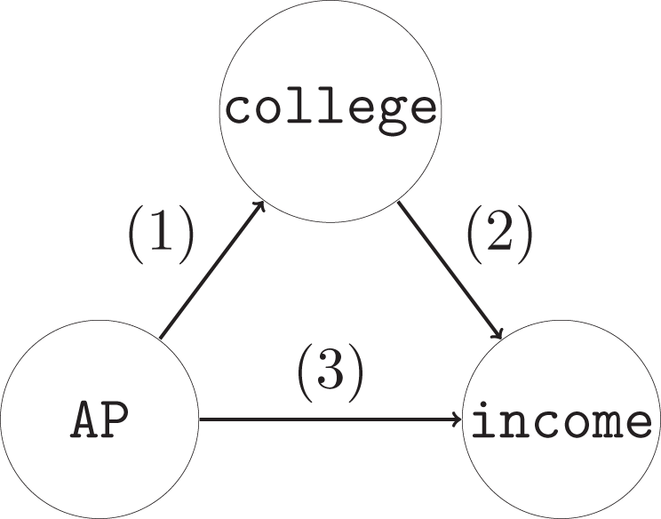
A schematic representation of mediation analysis, in which the treatment variable Z, in this case the variable AP, affects the outcome Y, in this case the variable logInc, via a mediator college and directly.

2. The Goals of Mediation Analysis: Defining Direct and Indirect Effects

Let Z denote a treatment of interest, and let Y denote an outcome. In a traditional causal inference study, each subject has a set of “potential outcomes”: Y(Z = z), for each z in the support of Z (Holland, 1986; Rubin, 1978; Splawa-Neyman, Dabrowska, & Speed, 1990). These record the outcome that a subject would present were she assigned to treatment z. Notably, Y(Z = z) is well defined for all subjects in the study but only observed for subjects whose treatment assignment was z.

In our AP program example, Z equals 1 for students who participated and 0 for others; so every student, in the treatment or the control arm, has two potential outcomes of this sort, Y(Z = 1) and Y(Z = 0). However, Y(Z = 1) is only observed for subjects in the intervention group, and Y(Z = 0) is only observed for subjects in the control group. Then subject i’s observed value is Y_i = Z_iY_i(Z = 1) + (1 − Z_i) Y_i (Z = 0). Each subject i’s treatment effect is Y_i (Z = 1) − Y_i (Z = 0); since we only observe one of Y(Z = 0) or Y(Z = 1), an individual’s treatment effect is typically unidentified. However, aggregate treatment effects, such as the average treatment effect (ATE) E[Y(Z = 1) − Y(Z = 0)], may be identified under certain conditions. Specifically, the ATE is identified when there is no interference between units—that is, a subject’s potential outcomes are functions of his or her treatment status Z_i and not the treatment status of other subjects—and no unobserved confounding—an unobserved variable that predicts both Z and Y(Z = 1), Y(Z = 0), or both, after conditioning on observed variables.

In the presence of a mediator M, for instance, college attendance, the potential outcomes framework needs to be expanded. Specifically, since M itself is a function of the treatment, M also has potential values M(Z = z). Furthermore, Y’s potential values may be written as a function of both Z and M, as Y(Z = z, M = m) or, more compactly, as Y(z, m). In fact, Y’s potential values can reflect M’s dependence on Z. So, for instance, Y_i(Z = 1, M = M(1)) = Y(Z = 1) is subject i’s log income if i participates in the AP encouragement program and exhibits resulting amount of schooling. Alternatively, Y_i(Z = 0, M = M(0)) = Y(Z = 0) is i’s log income if he does not participate in the program and receives the resulting amount of schooling. Adding M = M(z) to the potential outcomes for Y may seem redundant; however, it allows for strictly counterfactual outcomes—those that could never be observed but could still be rigorously defined. Specifically, Y_i(Z = 1, M = M(0)) represents subject i’s log income if i participates in the program but goes on to complete the amount of schooling he would have completed without the program, and Y_i(Z = 0, M = M(1)) is i’s log income if i does not participate in the program but attains the education he would have completed if he had participated.

The mediation software package is designed to estimate averages of two types of mediational effects, often called “causal mediation effects” and “direct effects.”¹ For a binary treatment Z, the causal mediation effect is either

δ (0) = Y (Z = 0, M = M (1)) - Y (Z = 0, M = M (0))

δ (1) = Y (Z = 1, M = M (1)) - Y (Z = 1, M = M (0)),

in which we imagine that Z is held fixed at either 0, as in δ(0), or 1, as in δ(1), but M is allowed to vary from what it would be under treatment M(1) to what it would be under control M(0). For instance, in the AP example, δ(0) is the effect, for subjects who do not participate in the program, of educational attainment varying as if they had attended the program. Say the AP program affects her income in several different ways, including causing her to attend college—having participated, she did attend, so M(1) = 1, but had she not participated, she would not have attended college, so M(0) = 0. Without participating in the AP program, she would not have been motivated to attend college, so M(0) = 0. But say the program also, by causing her to take an AP class, increased her confidence and analytical abilities, which improve her income regardless of her educational attainment. δ(0) is the effect in her income of attending college, if she has the confidence and analytical ability she would have without the AP program. δ(1) is the effect in her income of attending college, if she has confidence and analytical ability she would have if she does participate in the AP program. A difference between δ(0) and δ(1) is referred to as a “treatment-mediator interaction” and captures the difference of the effect of M in treatment or control conditions.

Direct effects, on the other hand, capture the effect of the treatment that does not depend on M. Analogous to δ(0) and δ(1), there are two types:

ζ (0) = Y (Z = 1, M = M (0)) - Y (Z = 0, M = M (0))

ζ (1) = Y (Z = 1, M = M (1)) - Y (Z = 0, M = M (1)) .

These hold the mediator value fixed at what it would have been under control (ζ(0)) or treatment (ζ(1)). For instance, in the AP example, ζ(0) is difference in our example subject’s log income if she gains the confidence and analytical ability from the AP program versus if she does not, assuming she does not attend college. ζ(1) is the same difference, if she does.

The mediation and direct effects add up to the total effect of the treatment:

\begin{matrix} ζ (1) + δ (0) = Y (Z = 1, M = M (1)) - Y (Z = 0, M = M (1)) + Y (Z = 0, M = M (1)) - Y (Z = 0, M = M (0)) \\ = Y (Z = 1, M = M (1)) - Y (Z = 0, M = M (0)) \\ = Y (Z = 1) - Y (Z = 0), \end{matrix}

with an analogous result for ζ(0) + δ(1). Mediation analysis, then, decomposes the effect of the treatment Z on the outcome Y into a portion dependent on M and one dependent on other mechanisms.

Just as individual treatment effects Y_i(1) − Y_i(0) are not typically identified, individual causal mediation effects and direct effects are not identified either. The mediation package, following most mediation analyses, focuses on estimating average causal mediation effects (ACMEs) and average direct effects (ADEs), or Eδ and Eζ. I will discuss the assumptions under which ACME and ADE are identified in the context of sensitivity analysis in Section 4. Briefly, in addition to no interference between units, mediation analysis requires no unmeasured confounding between the treatment and both the mediator and the outcome and no unmeasured confounding between the mediator and the outcome. To satisfy these conditions, it helps to condition analysis on pretreatment covariates X.

3. Estimating ACME and ADE in the mediation Package

Estimating average direct and indirect effects is a three-step procedure (Imai, Keele, Tingley, & Yamamoto, 2011). The first step is to estimate a distribution for M(z) for each treatment z, using a model of the mediator as a function of the treatment or f_M|Z. For the AP example, with college attendance college as a mediator, I used binary probit, implemented with the R function glm() as f_M|Z:

medModel <- glm(college∼AP+ses,family=binomial(probit), data=APdata)

I included ses, a continuous pretreatment covariate, in the model as well.

The next step fits a model for Y(Z, M), f_Y|M,Z, yielding a distribution for Y’s potential outcomes for each possible treatment z and mediator value m. In the AP example, I used ordinary least squares (OLS) regression, regressing logIncome on a combination of AP, college implemented with lm(), as f_Y|M,Z.

outModel <- lm(logIncome∼AP*college+ses,data=APdata)

This model also contains ses as well as allowing college to interact with AP—a treatment–mediator interaction.

Jointly, f_M|Z and f_Y|M,Z can estimate the quantities Y(1, M(1)), Y(1, M(0)), Y(0, M(1)), and Y(0, M(0)) for each subject—each subject’s potential log income if she participates or does not participate in the AP program and attends college as if she had attended, or not attended, college. These are the four quantities necessary for estimating δ and ζ. The final step estimates these quantities, and with them, δ and ζ.

Generally, the procedure is as follows: first, estimate f_M|Z and f_Y|M,Z from the data and then combine the fitted models with the mediate() function.

library(mediation)

med <- mediate(model.m = medModel,model.y = outModel,treat = ‘AP’, mediator = ‘college’,data=APdata)

Use the summary() function to display the results:

summary(med)

## Causal Mediation Analysis

## Quasi-Bayesian Confidence Intervals

##	Estimate 95%	CI Lower 95%	CI Upper	p-value
## ACME (control)	0.03204	0.00444	0.06595	0.02
## ACME (treated)	0.01833	0.00121	0.04405	0.04
## ADE (control)	0.16213	0.02843	0.29067	0.02
## ADE (treated)	0.14842	0.01043	0.27413	0.04
## Total Effect	0.18046	0.04306	0.31377	0.01
## Prop. Mediated (control)	0.17346	0.02259	0.69009	0.03
## Prop. Mediated (treated)	0.09315	0.00657	0.42898	0.04
## ACME (average)	0.02518	0.00342	0.05129	0.02
## ADE (average)	0.15527	0.02143	0.28245	0.02
## Prop. Mediated (average)	0.13331	0.01924	0.54994	0.03

## Sample Size Used: 1000

## Simulations: 1000

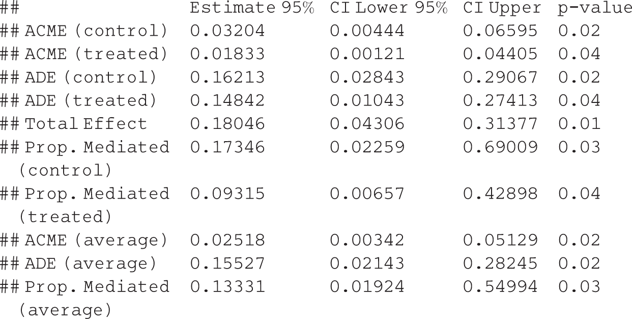
The model detected both natural direct and indirect effects. Since the outcome model I specified, f_Y|M,Z, included an interaction between AP and college, the model looked for differences between δ(0) and δ(1), the mediated effect holding AP constant at 0 or 1, respectively. The ACME for students who are not in the AP intervention was estimated as between 0.004 and 0.066, in effect size units, with 95% confidence. For students in the intervention, the confidence interval was [0.001, 0.044].

The summary function also displays results for the ADE, estimated as [0.028, 0.291] or [0.01, 0.274] in the control and intervention groups, respectively, and the total effect, estimated as [0.043, 0.314]. Finally, perhaps the most interpretable measure of mediation is the “proportion mediated,” which is the proportion of the total effect explained by the mediator, or δ(0)/(δ(0) + ζ(1)) or δ(1)/(δ(0) + ζ(1)). For control subjects, this proportion is between 0.023 and 0.69, and for treated students, the proportion is between 0.007 and 0.429.

It is also possible to plot 95% confidence intervals for the ACME, ADE, and total effect, as in Figure 2.

Figure 2.

Estimates (points) and 95% confidence intervals for the average causal mediation effect (ACME), average direct effect (ADE), and total effect. The solid points and lines represent ACME and ADE for the treatment group, and the dotted lines and empty points represent estimates for the control group.

In principle, any models that yield estimates of M or Y as a function of Z or Z and M, respectively, would be compatible with potential outcomes framework for mediation analysis. In practice, the mediate routine is compatible with a very wide range of options within R. A complete list of compatible models is available in Tingley et al. (2014, p. 5); in brief, linear models, generalized linear models (GLMs), ordered probit models, generalized additive models (GAMs), quantile models, or survival models, with one or two levels, are compatible for f_M|Z or f_Y|M,Z. Additionally, f_Y|M,Z may be modeled as tobit.

Options in the mediate() command allow robust (sandwich), cluster robust, and bootstrap standard errors. It also allows the user to specify values of a continuous treatment variable to contrast.

4. Identification Assumptions and Sensitivity to Hidden Bias

Causal mediation analysis requires stronger assumptions than traditional causal inference, one of which is untestable even in conventional randomized controlled trials.² In addition to assuming no interference between units, as discussed in Section 2, analysts must also assume that there is no unmeasured confounding. Specifically, mediation analysis requires sequential ignorability (Imai, Keele, & Yamamoto, 2010):

Y_{i} (z, m) ╨ Z_{i} | X_{i},

M_{i} (z) ╨ Z_{i} | X_{i},

Y (z^{'}, m) ╨ M_{i} (z) | Z_{i}, X_{i} .

The first two ignorability assumptions, Equations 5 and 6, are familiar from conventional causal inference—in order to infer the effect of Z on M or Y, Z must be independent of M and Y’s potential outcomes, conditional on observed covariates X. Equations 5 and 6 are satisfied in randomized trials, where the researcher controls distribution of Z.

The third part of the assumption, Equation 7, is necessary to infer the effect of M on Y. It posits that, conditional on realized treatment Z = z and covariates, M is independent of Y’s potential outcomes. Randomizing Z, as in conventional randomized trials, does not guarantee that Equation 7 is satisfied. Indeed, since the effect of Z on M is a crucial piece of mediation analysis, directly manipulating M would be undesirable.

Figure 3 gives an interpretation of sequential ignorability in terms of unmeasured confounders U₁, U₂, and U₃ which would violate it. If an unmeasured variable predicts both Z and M, such as U₁, both M and Y, such as U₂, or both Z and Y, such as U₃, sequential ignorability does not hold. Importantly, U₂ may be pre- or posttreatment—in either case, it will violate sequential ignorability and bias the mediation analysis. The three omitted variables in Figure 3 map on to the three equations that comprise sequential ignorability: U₁ violates Equation 5, U₂ violates Equation 7, and U₃ violates Equation 6. As above, then, randomization of Z implies that there are no variables such as U₁ and U₃ that could confound the analysis; however, a confounder such as U₂ is harder to control. The fact that U₂ may be posttreatment is especially troubling, since even if it were measured, adjusting the analysis for a posttreatment U₂ is nontrivial and requires further untestable assumptions.

Figure 3.

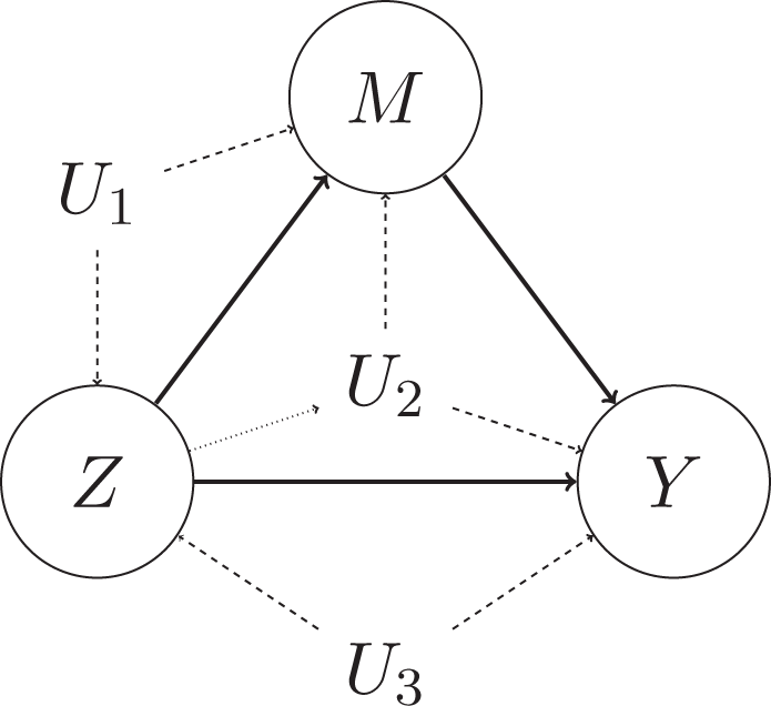
A graph of three different types of confounding variables, which may violate sequential ignorability. U₁ confounds the relationship between Z and M, U₂ confounds the relationship between M and Y, and U₃ confounds the relationship between Z and Y. The dotted line from Z to U₂ indicates that the confounder U₂ may be posttreatment.

The mediation package provides a function, medsens(), for researchers to assess the sensitivity of their mediation analyses to the assumption in Equation 7. The method applies when both f_M|Z and f_Y|M,Z are fit with OLS (using lm) or binary probit regression (using glm), two models that involve error terms. Then the idea behind the sensitivity analysis, described more fully in Imai, Keele, and Yamamoto (2010), is that an unobserved pretreatment confounder between M and Y, such as U₂, would induce a correlation between the errors f_M|Z and f_Y|M,Z. In fact, knowing the correlation between errors, denoted ρ, would suffice to estimate the ACME and ADE without bias. The sensitivity analysis reestimates the ACME and ADE for a vector of values for ρ; the set of ACME estimates corresponding to plausible values of ρ captures the uncertainty in the estimated ACME due to violations of Assumption (7). The interval containing the 95% confidence bounds for the same set of plausible ρ values is a “sensitivity interval” (cf. Small, 2007), which accounts for uncertainty both due to sampling or randomization error and due to violations of Equation 7.

Choosing plausible values for ρ is a difficult task, since it depends wholly on substantive theory and prior research—the data themselves are not informative. Moreover, ρ is a difficult parameter to interpret. However, Imai, Keele, and Yamamoto (2010), along with the output from medsens(), provide two alternative parameterizations that may be easier to interpret. The two alternatives take the form of the product of two coefficients of determination (R²) values. One, denoted as $R_{M}^{2 *} R_{Y}^{2 *}$ , is the product of the amount of previously unexplained variation in M and Y due to a missing confounder. The second, denoted as ${\tilde{R}}_{M}^{2} {\tilde{R}}_{Y}^{2 *}$ , is the product of the amount of total variation in Y and M explained by a missing confounder. Converting between the ρ formulation and the $R_{M}^{2 *} R_{Y}^{2 *}$ formulation is simple: $R_{M}^{2 *} R_{Y}^{2 *}$ is equal to ρ².

With a fitted mediation model in hand, such as med, above, conducting such a sensitivity analysis in mediation is straightforward:

sensitivityAnalysis <- medsens(med)

The output from medsens() can be displayed via the summary() command, which returns the values of ρ,

R_{M}^{2 *} R_{Y}^{2 *}

, and

{\tilde{R}}_{M}^{2} {\tilde{R}}_{Y}^{2 *}

at which the ACMEs for the treatment and control group are approximately 0.

summary(sensitivityAnalysis) ## ## Mediation Sensitivity Analysis: Average Mediation Effect ## ## Sensitivity Region: ACME for Control Group ##
## Rho	ACME (control)	95% CI Lower	95% CI Upper	R⁁2_MR⁁2_Y	R⁁2_M∼R⁁2_Y∼
## [1,] 0.2	0.0101	−0.0037	0.0318	0.04	0.0124
## [2,] 0.3	−0.0003	−0.0155	0.0152	0.09	0.0279
## [3,] 0.4	−0.0107	−0.0306	0.0035	0.16	0.0497
## ## Rho at which ACME for Control Group = 0: 0.3 ## R⁁2_MR⁁2_Y at which ACME for Control Group = 0: 0.09 ## R⁁2_M∼R⁁2_Y∼ at which ACME for Control Group = 0: 0.0279 ## ## ## Sensitivity Region: ACME for Treatment Group ##
## Rho	ACME (treated)	95% CI Lower	95% CI Upper	R⁁2_MR⁁2_Y	R⁁2_M∼R⁁2_Y∼
## [1,] 0.1	0.0076	−0.0060	0.0257	0.01	0.0031
## [2,] 0.2	−0.0039	−0.0230	0.0108	0.04	0.0124
## [3,] 0.3	−0.0140	−0.0363	0.0003	0.09	0.0279
## ## Rho at which ACME for Treatment Group = 0: 0.2 ## R⁁2_MR⁁2_Y at which ACME for Treatment Group = 0: 0.04 ## R⁁2_M∼R⁁2_Y∼ at which ACME for Treatment Group = 0: 0.0124

Users can also plot the sensitivity as in Figure 4. Figure 4 shows how the point estimates (solid line) and confidence intervals for δ(0) and δ(1) vary as a function of ρ. The dotted line indicates estimates and confidence intervals for δ when sequential ignorability holds and ρ = 0.

Figure 4.

Sensitivity analysis for causal mediation.

Alternatively, users can directly access the sensitivity results to compute sensitivity intervals or other analysis summaries. For instance, an education researcher may hypothesize a particularly problematic unmeasured covariate (ambition, say) and argue that it is implausible that it accounts for more than 25% of the unexplained variation in either college attendance or log income. Then, she may use the following code to compute a sensitivity interval assuming $R_{M}^{2 *} R_{Y}^{2 *} = ρ^{2} < 0.25$ :

## ACME for the control group:

with(sensitivityAnalysis,

print(c(min(lower.d0[rho⁁2<0.25]),max(upper.d0[rho⁁2 <0.25]))))

## [1] −0.03064665 0.13562650

## ACME for the treatment group:

with(sensitivityAnalysis,

print(c(min(lower.d1[rho⁁2<0.25]),max(upper.d1[rho⁁2 <0.25]))))

## [1] −0.05102738 0.11427861

The sensitivity analysis of the toy AP data suggests that its estimates are rather sensitive to hidden bias; unless theoretical or background knowledge rules out mediator-exposure confounders of all but minimal importance, the interpretation of the mediation analysis must be conservative.

The focus of mediation’s sensitivity analysis on mediator-outcome confounding, such as U₂, follows most of the causal mediation literature—though an appendix of VanderWeele (2010) provides a method for treatment-mediator confounding. This is presumably because treatment-mediator or treatment-outcome confounding is controllable via a randomized experiment. However, in education sciences, observational studies predominate and a method for assessing sensitivity to confounders of all types would be useful.

5. Moderated Mediation

It is possible for direct and indirect effects to depend on a pretreatment covariate X. For instance, in our AP example, the AP intervention may have a larger effect on college attendance for low-SES students than for high-SES students. Then the natural indirect effect δ would depend on X, as δ(z, X). This is referred to as “moderated mediation.” The mediation package provides a method to estimate moderated mediation, via the covariates argument in the mediation() function. To demonstrate, I will first refit f_M|Z to include an interaction between AP and ses. Then, I will estimate two ACMEs, at the first and third quantiles of the empirical SES distribution, to examine the dependence of δ on SES. The code and results can be found in Figure 5.

Figure 5.

Estimating mediational effects at high and low SES: Moderated mediation.

6. Limitations

The mediation package is invaluable for researchers interested in mediation. That said, the development of the mediation must be an ongoing project (and I believe it is). Quantitative education research relies heavily on path analysis and linear structural equation modeling (SEM) using programs such as Mplus (Muthén and Muthén, 1998–2012) or R packages such as lavaan or sem (Fox, Nie, & Byrnes, 2015; Rosseel, 2012) that do not take full advantage of the recent methodological advances in causal mediation analysis. One advantage of the SEM framework is that it can incorporate latent variables and measurement models into analyses, complications that, to the best of my knowledge, are not yet in the purview of potential outcomes-based mediation methodology. But the other advantage of SEM software is its ability to model highly complex mediational models, with several causally dependent mediators and moderators. There has been some recent work on identification and estimation for multiple mediators in the potential outcomes framework, such as Imai and Yamamoto (2013) and VanderWeele and Vansteelandt (2013); if these methods were incorporated into the mediation package, it would be even more valuable to the education research community.

Another valuable addition would be options for sensitivity analysis for data from observational studies, as described above. Although randomized experiments are becoming more common in the social sciences, they are still not the norm, so accessible sensitivity analysis methods for observational studies could prove very useful.

Finally, the mediation software can take a long time to run, and there are several places in the source code that can be modified to speed things up. For instance, some aspects of the mediation computation are embarrassingly parallel—modifications to the software that would allow for parallel computation would improve matters.

7. Conclusion

The past decade of research has made mediation analysis rigorous, flexible, and conceptually sound. However, many of the newer mediation methods can be difficult to implement, especially when either M or Y is nonnormal, or relationships are nonlinear. Additionally, the strong untestable assumptions in mediation analysis make sensitivity analysis indispensable; this adds even further to the difficulty of implementing a careful mediation study. All that being the case, the mediation package is an invaluable addition to the educational and behavioral statistics tool kit. The mediate() function is easy to implement, and its output is (relatively) easy to understand. It is extremely flexible in terms of the outcome and mediation models it takes as inputs, which allows researchers to model the data as they see fit, instead of having to contort their data analysis into one of a few forms. Further, the fact that it takes fitted models as inputs, instead of raw data and instructions, allows researchers to select the model that they feel best represents the data, using all available model fit criteria, before beginning the mediation analysis. The sensitivity function medsens() is similarly easy to use, and the plots it generates are both visually appealing and highly interpretable—at least as far as sensitivity analysis plots go.

Mediation analysis is one of the more exciting new developments in statistical causal inference. The mediation package, with its ease of use and flexibility, grants quantitative researchers access to the new methods to a wide range of quantitative researchers.

Footnotes

Declaration of Conflicting Interests

The author(s) declared no potential conflicts of interest with respect to the research, authorship, and/or publication of this article.

Funding

The author(s) received no financial support for the research, authorship, and/or publication of this article.

Notes

References

Fox

Nie

Byrnes

(2015). sem: Structural equation models (R package version 3.1-6). Retrieved from https://CRAN.R-project.org/package=sem.

Holland

P. W.

(1986). Statistics and causal inference (with discussion). Journal of the American Statistical Association, 81, 945–970.

Hong

(2010). Ratio of mediator probability weighting for estimating natural direct and indirect effects. In JSM Proceedings (pp. 2401–2415), Biometrics Section. Alexandria, VA: American Statistical Association.

Hong

(2015). Causality in a social world: Moderation, mediation and spill-over. West Sussex: John Wiley.

Imai

Keele

Tingley

Yamamoto

(2009). Causal mediation analysis using R. In Vinod

H. D.

(Ed.), Advances in social science research using R (pp. 129–154). New York, NY: Springer.

Imai

Keele

Yamamoto

(2010). Identification, inference and sensitivity analysis for causal mediation effects. Statistical Science, 25, 51–71.

Imai

Keele

Tingley

Yamamoto

(2011). Unpacking the black box of causality: Learning about causal mechanisms from experimental and observational studies. American Political Science Review, 105, 765–789.

Imai

Tingley

Yamamoto

(2013). Experimental designs for identifying causal mechanisms. Journal of the Royal Statistical Society: Series A (Statistics in Society), 176, 5–51.

Imai

Yamamoto

(2013). Identification and sensitivity analysis for multiple causal mechanisms: Revisiting evidence from framing experiments. Political Analysis, 21, 141–171.

10.

Muthén

L. K.

Muthén

B. O.

(1998–2012). Mplus user’s guide. Seventh edition. Los Angeles, CA: Muthén & Muthén.

11.

R Development Core Team. (2011). R: A language and environment for statistical computing. Vienna, Austria: R Foundation for Statistical Computing. Retrieved from http://www.R-project.org/.ISBN3-900051-07-0

12.

Rosseel

(2012). lavaan: An R package for structural equation modeling. Journal of Statistical Software, 48, 1–36. Retrieved from http://www.jstatsoft.org/v48/i02/

13.

Rubin

D. B.

(1978). Bayesian inference for causal effects: The role of randomization. The Annals of Statistics, 6, 34–58.

14.

Small

D. S.

(2007) Sensitivity analysis for instrumental variables regression with overidentifying restrictions. Journal of the American Statistical Association, 102, 1049–1058.

15.

Splawa-Neyman

Dabrowska

D. M.

Speed

T. P.

(1990). On the application of probability theory to agricultural experiments. Essay on principles. Section 9. Statistical Science, 5, 465–472.

16.

Tingley

Yamamoto

Hirose

Keele

Imai

(2014). mediation: R package for causal mediation analysis. Journal of Statistical Software, 59, 1–38. doi:10.18637/jss.v059.i05. Retrieved from https://www.jstatsoft.org/index.php/jss/article/view/v059i05

17.

VanderWeele

T. J.

(2008). Simple relations between principal stratification and direct and indirect effects. Statistics & Probability Letters, 78, 2957–2962.

18.

VanderWeele

T. J.

(2010). Bias formulas for sensitivity analysis for direct and indirect effects. Epidemiology (Cambridge, Mass.), 21, 540.

19.

VanderWeele

T. J.

(2014). A unification of mediation and interaction: A 4-way decomposition. Epidemiology (Cambridge, Mass.), 25, 749–761.

20.

VanderWeele

T. J.

(2015). Explanation in causal inference: Methods for mediation and interaction. Oxford, England: Oxford University Press.

21.

VanderWeele

T. J.

Vansteelandt

(2013). Mediation analysis with multiple mediators. Epidemiologic Methods, 2, 95–115.