
Abstract
Classroom interactions between students and teachers form a two-way or dyadic network. Measurements such as days absent, test scores, student ratings, or student grades can indicate the “quality” of the interaction. Together with the underlying bipartite graph, these values create a valued student–teacher dyadic interaction network. To study the broad structure of these values, we propose using interaction factor analysis (IFA), a recently developed statistical technique that can be used to investigate the hidden factors underlying the quality of student–teacher interactions. Our empirical study indicates there are latent teacher (i.e., teaching style) and student (i.e., preference for teaching style) types that influence the quality of interactions. Students and teachers of the same type tend to have more positive interactions, and those of differing types tend to have more negative interactions. IFA has the advantage of traditional factor analysis in that the types are not presupposed; instead, the types are identified by IFA and can be interpreted in post hoc analysis. Whereas traditional factor analysis requires one to observe all interactions, IFA performs well even when only a small fraction of potential interactions are actually observed.
Interactions between students and teachers lie at the core of the education process (Cohen & Ball, 1999). A growing body of literature suggests the effect of personal variables other than the more traditionally studied variables of teacher quality, didactic aptitude, and credentials or student academic ability that can significantly impact the quality of interactions between students and teachers. For example, Duffy, Warren, and Walsh (2001) indicate that female math teachers tend to be more responsive to male students, whereas Jones and Wheatley (1990) suggest that female science teachers are more likely to give male students behavioral warnings in the classroom under the Brophy–Good Teacher–Child Dyadic Interaction System (Good & Brophy, 1972). Saft and Pianta (2001) show evidence of a positive interaction in the Student–Teacher Relationship Scale (STRS) if the student–teacher dyad is of the same ethnicity. Most recently, research on the intellectual styles suggests that a match in the teaching and learning styles between the student and teacher can lead to a positive classroom relationship and learning outcome (Witkin, 1973; Zhang, 2006). Such work suggests the potential for latent factors that are underlying the quality of student–teacher interactions.
Measurement of teacher–student interactions can also have implications for teacher value-added modeling. In value-added modeling, the effectiveness of individual teachers is quantified on the basis of student test scores, often with the effects of particular student covariates controlled. As discussed by Lockwood and McCaffrey (2009), significant student–teacher interactions may call into question the meaningfulness of teacher value-added estimates, on the one hand, as teacher effects will be expected to vary depending on the student. Interactions may also provide useful information for improving teacher effectiveness, either by providing a basis for improved classroom assignments of students to teachers or through targeted teacher interventions focusing on specific areas for teacher improvement. Prior work attending to student–teacher interactions has examined variability in teacher effects in relation to known (or directly measurable) student characteristics, such as prior or predicted achievement levels, race/ethnicity, or gender. A unique feature of the proposed methodology is its potential to identify such interactions without a priori student or teacher variables. As will be shown, the methodology shares similarities with exploratory factor analysis (EFA), whereby factors can be detected and used even though they may not be perfectly aligned with other variables, in this case, student or teacher covariates.
Which factors are most relevant in determining the quality of an interaction? Do these factors vary between schools and settings? By using various forms of linear regression, previous research prescribed which factors have the potential to determine the quality of an interaction. The quality of this interaction could be measured by a metric on the student following exposure to the teacher.
However, given the wide range of potential factors in determining successful interactions and the inability to measure many of them, we propose a method that estimates the factors from the data instead of testing a priori. For example, if one measures the quality of every student–teacher interaction, then traditional statistical modalities such as EFA or principal component analysis (PCA) would produce such results. Then, the factors could be identified in post hoc analysis. Interestingly, such an analysis allows for the results to change from one school to the next; perhaps teaching style is important for one student–teacher population, while gender matching is important for another population.
EFA and PCA are not feasible in most American schools because each student only interacts with a small proportion of the teachers in his or her school. This leaves several student–teacher interactions unmeasured. In this article, we overcome this practical constraint by employing low-rank matrix completion (a type of content recommendation or collaborative filtering).
This collection of techniques gained popularity from the Netflix prize (Feuerverger, He, & Khatri, 2012) and is used throughout web commerce to produce product recommendations based upon users’ preferences in the past. In web commerce, low-rank matrix completion studies the valued dyadic interaction network between customers and products; here, the “values” come from implicit or explicit product ratings. For example, at Amazon.com, customers browse products and potentially purchase the product. Using Netflix, customers view and potentially rate the movies. Based on this information, the commercial websites recommend further products for each customer using content recommendation algorithms. In some situations, the recommendation algorithm is built on multivariate statistical tools that are akin to EFA and PCA. As such, they infer types of users and types of products. Koren, Bell, and Volinsky (2009, p. 35) describe the Netflix factors thusly:
The first factor has on one side lowbrow comedies and horror movies, aimed at a male or adolescent audience (Half Baked, Freddy vs. Jason), while the other side contains drama or comedy with serious undertones and strong female leads (Sophie’s Choice, Moonstruck). The second factor has independent, critically acclaimed, quirky films (Punch-Drunk Love, I Heart Huckabees) on one side, and mainstream formulaic films (Armageddon, Runaway Bride) on the other side.
Following the models used in web commerce, we view the school as a valued dyadic interaction network in which each interaction between the student and teacher is given a quality metric. In turn, we can adapt the above low-rank matrix completion methodology to study the student–teacher interactions. While in its application to web commerce, low-rank matrix completion is primarily used for the purpose of prediction; one of its intermediate steps is to estimate the latent factors underlying each interaction. Inspired by this approach, we develop interaction factor analysis (IFA) to study the valued interaction networks of students and teachers. Despite potentially many missing values, IFA can systematically determine the hidden factors that impact student–teacher interaction. These latent factors could correspond to gender, learning/teaching styles, or thinking patterns of the student–teacher dyad. In addition to inferring the latent dimensions of student–teacher interactions, at a very practical level, IFA has the merit in recommending which students and teachers will have the most successful interactions. For example, if IFA determines that the “types” correspond to auditory, visual, and kinesthetic learning (Dunn, Dunn, & Price, 1989; Kolb, 1999), then IFA will determine the learning and teaching style of each student and teacher and produce a recommendation that matches styles. Similar to EFA, IFA does not presuppose what the latent factors represent. Instead, the types that are estimated from the data can be interpreted in a post hoc analysis. In this case, one could determine whether the latent factors align with previously measured covariates or whether they correspond to something that has yet been measured.
The next section gives readers an overview of the valued dyadic network of student–teacher interactions and proposes a latent factor model. The sections that follow provide details about using IFA to estimate the parameters in the model and illustrate IFA applied on an artificial data set. The final sections illustrate the methodology on data taken from a secondary school in the state of Florida.
The Valued Dyadic Network of Student–Teacher Interactions
To understand the underlying idea of IFA applied to education research, first imagine a school where every student is exposed to every teacher. For each student–teacher dyad, there is a metric that represents how well the student performed with the teacher. Arrange these scores into a matrix
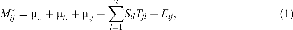
where μ.. is the mean score of all the students in the school, μi. is the expected deviation of student i from the grand mean μ.., μ.j is the expected deviation of teacher j from the grand mean μ.., and Eij is the (i, j) th entry of matrix
This article focuses on the matrices S and T; their columns represent different qualities of students and teachers and determine the expected outcome of the student–teacher interaction. For simplicity, the fixed effects will be presumed to be to 0 throughout the next two sections on Method and Simulations. The subsequent section on Numerical Analysis will account for the fixed effects.
EFA applied to the fully observed M* can estimate S and T to investigate latent factors that underlie the student–teacher interaction. However, in most American schools, many student–teacher interactions are unobserved. Instead of observing M*, we observe
Our Method
IFA will succeed in estimating S and T when κ is much less than
Background on the Eigendecomposition and the Singular Value Decomposition (SVD)
The eigendecomposition and the SVD are fundamental topics in linear algebra. Both IFA and, more classically, EFA employ these techniques. The most common method for computing the loading factors in EFA is initialized through the eigendecomposition on the correlation matrix (Harman, 1976). Given the fully observed matrix M*, we center and scale M* so that each column of the new matrix has mean 0 and variance 1 and call this matrix Z. If the rows of M* are iid draws from a multivariate distribution, then

where Δ is a diagonal matrix whose diagonal elements
Let
where

EFA uses
The SVD is closely related to the eigendecomposition. The SVD of the centered and column-scaled matrix Z yields
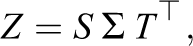
where

The next section shows how this SVD formulation nicely extends to IFA. Where the SVD computes the RSS over all pairs (i, j) in the matrix Z, the optimization problem for IFA will only sum over the observed pairs
Interaction Latent Factor
In a typical American school, we only observe M, which is a sparsely observed matrix. For a single school, let

is not computationally tractable. The above optimization problem is nonconvex, and only heuristic algorithms exist (Srebro & Jaakkola, 2003).
The standard approach to this computational problem is similar to the approach taken by the Lasso (Tibshirani, 1996). In model selection for linear regression, the Lasso does not optimize over all models with κ terms in the model. Instead, it relaxes this optimization problem, replacing the “κ terms” optimization constraint with a convex penalty.
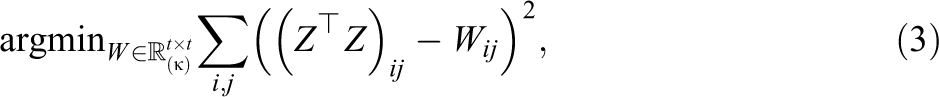
Similarly, instead of restricting the IFA optimization routine to rank κ matrices, an extended literature on low-rank matrix completion studied an analogous convex relaxation for Equation 5, where the explicit rank constraint is replaced by the nuclear norm penalty
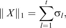
where σls are the singular values of X. This leads to the convex problem

where γ ≥ 0 is a tuning parameter (Candès & Tao, 2010). Notice that instead of restricting
The nuclear norm is responsible for making
Previous papers studied the theoretical properties of IFA. Appendix B gives an overview of the literature.
The Soft-impute Algorithm
The optimization problem in Equation 6 is a convex problem (Candès & Recht, 2009). As such, we can find the global optimum with the Step 0 (Initialization): Start with matrix M, fill in the missing observations with the average value of the observed elements to get Step 1: Given Step 2: Retain the top singular values Step 3: Impute the missing values of M with corresponding values of Step 4: Check if

for some ε > 0. The algorithm stops if the threshold condition in Equation 7 is met. Otherwise, increase h by 1 and repeat Steps 1 through 4.
The final left and right column vectors
Illustration on Simulated Data Sets
The Setup
Suppose our school includes 1,000 students and 100 teachers. On average, a student interacts with approximately 15% 4 of teachers. For each of those interactions, we can assign an interaction score. Thus, our interaction matrix M has 1,000 rows and 100 columns with approximately 15% of the entries present and 85% missing. Our observed interaction matrix M has s = 1,000 rows, t = 100 columns, and proportion of the teachers that each student takes classes with p = .15 in this case.
We further assume that the interaction quality between a student and teacher pair is influenced by three factors (k = 3): The student and teacher visual learning styles—students who are visual learners will interact well with teachers who rely on visual lecturing methods to deliver the materials, The student socioeconomic status (SES) and the teacher experience—teachers who have more years of experience will interact better with the students who are from lower socioeconomic backgrounds, and The student and teacher gender—the student–teacher pairs of the same gender will interact better than those of opposite genders. Lastly, the nature of these latent factors is stationary over time—a student’s preference does not change as he or she advances through the classes.
For the first student factor, which corresponds to the inclination of the student toward visual learning, we generate Si1 from a normal distribution centered at 0. For the second student factor, we use the probability that the student receives free or reduced-price lunch as a proxy for his or her SES. Si2 is generated from the standard uniform distribution. The third student factor, gender, Si3, is generated from Bernoulli distribution of equal probability to be male or female. Similarly, the first teacher factor Tj1 is generated from a normal distribution centered at 0, the second Tj2 from normal distribution, and third Tj3 from Bernoulli distribution.
Given the sparse interaction matrix M, we will investigate: (a) How the estimated latent factors influence the student–teacher interaction outcome in the same manner as the actual latent factors, (b) the relationship between the estimated latent factors and the actual ones, and (c) the optimal classroom assignment estimated using the imputed interaction matrix.
The Estimated Latent Factors
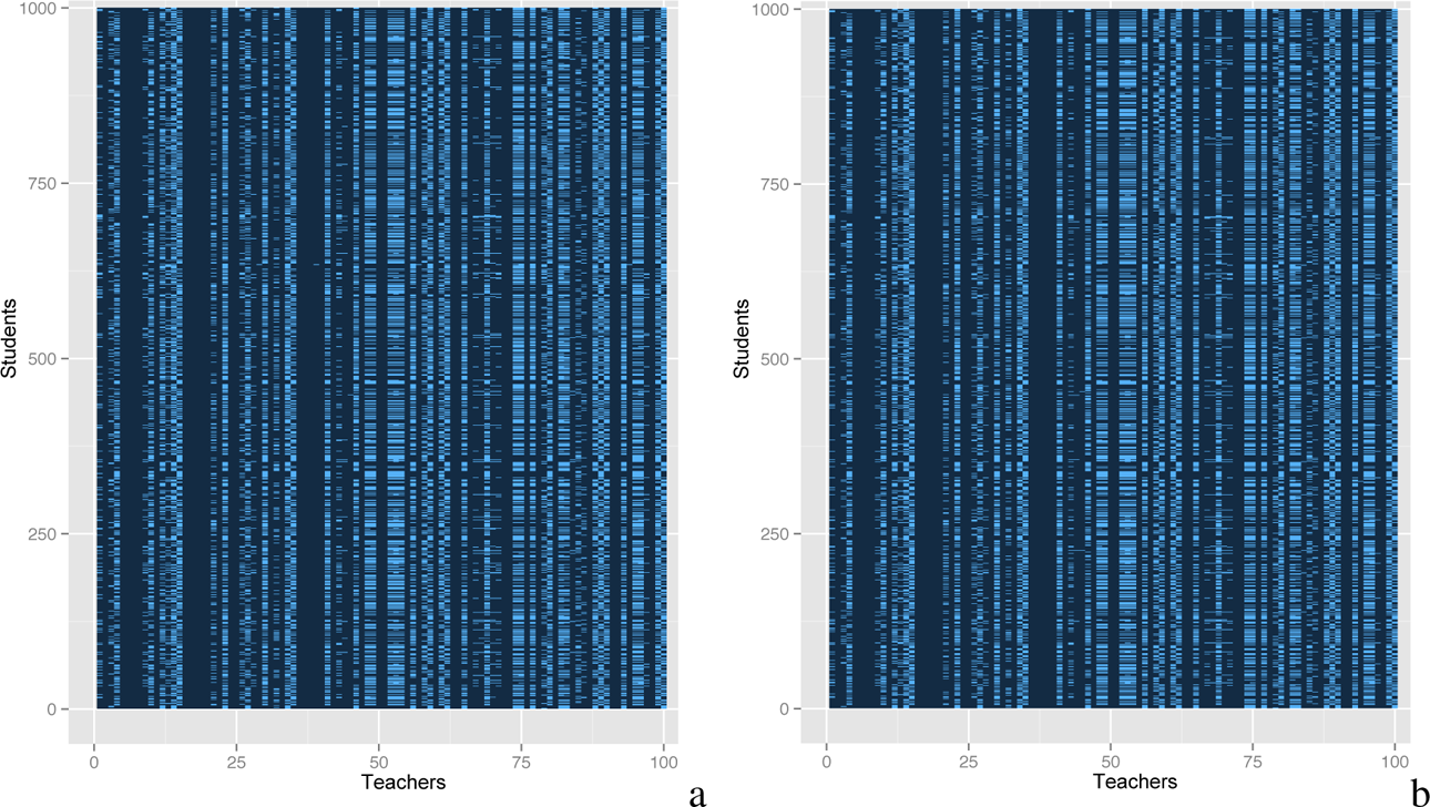
For the fully observed interaction matrix M*, we would expect that students who score high on visual learning will have high-quality interactions with teachers who score high on visual teaching; likewise, students from the lower end of the visual learning spectrum will have high-quality interactions with teachers from the lower end of the visual teaching spectrum. In contrast, students and teachers who are from two different ends of the visual teaching and learning spectrums will have lesser quality interactions. Thus, if we rearrange M* according to the visual learning and teaching scores of the students and teachers, there will be a pattern, which is shown in Figure 1a—a heat map of the rearranged M*. The brighter shades indicate higher interaction scores and vice versa. As we can see, the bottom left and top right corners have the brightest shades indicating the student–teacher pairs of the same visual teaching and learning styles, while the bottom right and top left corners have darkest shades indicating student–teacher pairs of opposite visual teaching and learning styles. Figure 1b is the heat map of the rearranged M* by the students’ probabilities of receiving free or reduced-price lunch and the teachers’ years of experience. The brighter shades at the top right corner indicate that students with high probabilities of receiving free or reduced-price lunch will interact well with more experienced teachers, and darker shades at the top left corner indicate that these same students will have lower interaction scores with less experienced teachers. Lastly, Figure 1c is the heat map of the rearranged M* by student and teacher gender. Again, there is a clear pattern of students and teachers of the same gender interacting well, while the opposite is true for students and teachers of different genders.
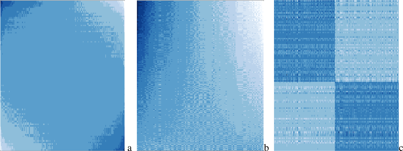
Heat map of student–teacher interaction matrix M* arranged by actual first, second, and third latent factors.
Now, instead, we are given the partially observed matrix M. In this case, IFA will help us estimate the latent factors, the columns of
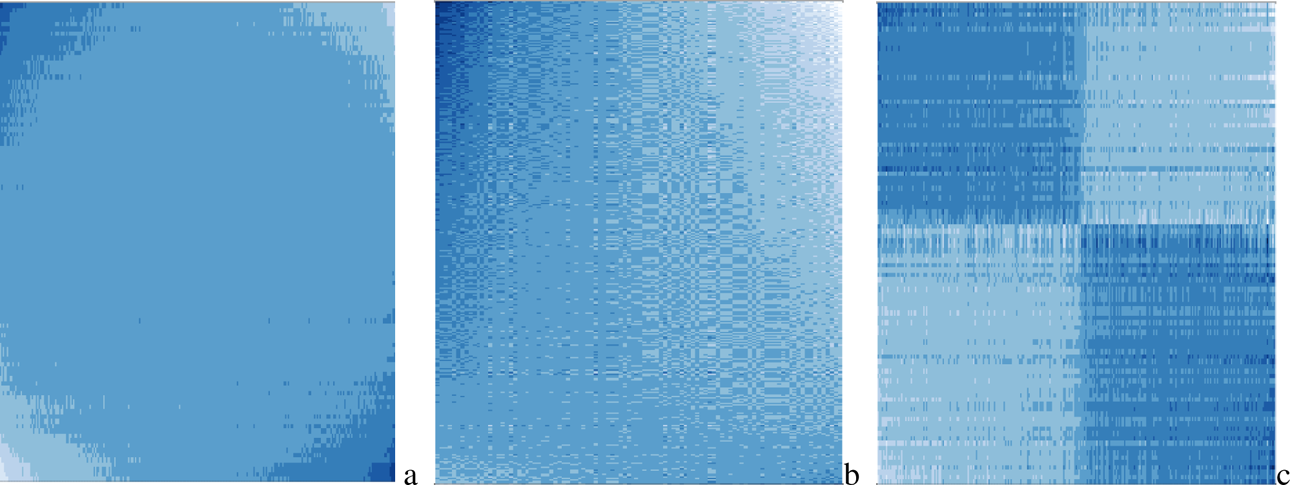
Heat map of student–teacher interaction matrix
Even more surprisingly, if we rearrange
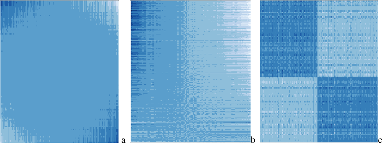
Heat map of student–teacher interaction matrix
All of the above indicate that IFA can efficiently recover the latent factors from a sparsely observed interaction matrix.
Canonical Correlations (CCs) Between the Actual Latent Factors and Estimated Ones
To explicitly explore the relationship between the actual latent factors and the estimated ones, we perform CC analysis (CCA) on these two sets of factors. Over 100 simulations, with only 15% of the student–teacher interactions observed, the CCs between the actual student latent factors and the estimated ones are averaged at .999, .980, and .810. Moreover, a closer look at the weight of each latent factor in making up the CC variables shows that the first actual latent factor (student visual learning style) is dominant in making up the first CC variable, the second actual latent factor (student SES), the second CC variable, and the third actual latent factor (student gender), the third CC variable. On the response side of the CCA, we have the same pattern. Figure 4 illustrates this phenomenon.
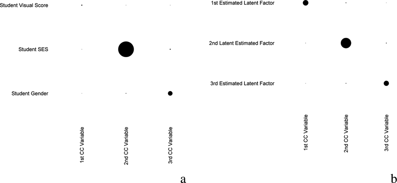
Weights of the student latent factors contributed to the canonical correlation variables.
Similarly, CCs between the actual teacher latent factors and the estimated ones are averaged at .999, .999, and .942. Also, each CC variable is mainly made up of one individual latent factor, as shown in Figure 5.
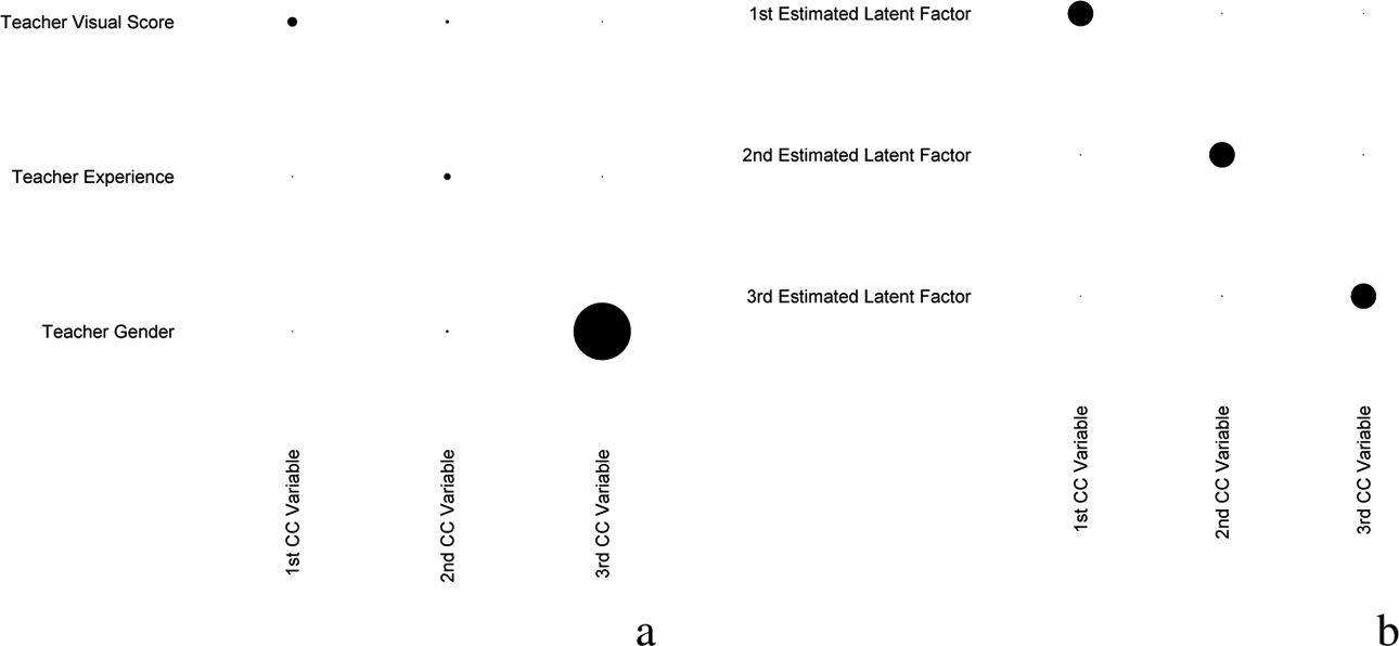
Weights of the teacher latent factors contributed to the canonical correlation variables.
Furthermore, we can show that the CCs between the actual latent factors and the estimated ones consistently increase as the proportion of observed interactions p increases. Given s = 1,000 and t = 100, we expect that IFA would reasonably recover the first student and teacher latent factors if p > .011, the second latent factors if p > .022, and the third latent factor if p > .033. 5
In practice, as it is shown in Figure 6, for student latent factors, the first CC reaches relatively high value when p = .011, second p = .1, and third p = .15. For teacher latent factors, the first CCs reach relatively high value as p = .011, second p = .033, and third p = .15. One of the reasons that IFA needs more observations in practice is because of the cold case imputing situation. When the proportion of observed interactions is relatively small, with high chance, there are students and teachers in our matrix with 0 or 1 observations, making it impossible for IFA to recover the latent factors. Nevertheless, in this setting, once the proportion of the observed interactions p reaches .15, IFA will almost perfectly recover the student and teacher latent factors.
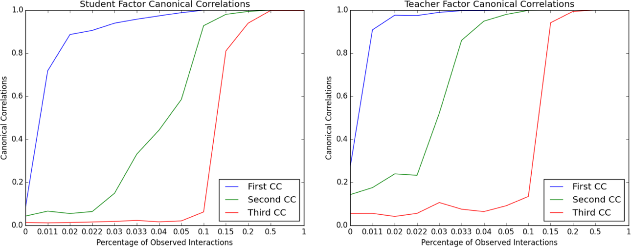
Student and teacher canonical correlations as functions of percentage of observed interactions.
The Optimal Classroom Assignment
One imminent application of IFA would be classroom assignment recommendations for students and teachers. We would question whether IFA applied on the sparsely observed M can reconstruct an optimal student–teacher assignment strategy that is reasonably similar to the one obtained from the fully observed M*.
In this experiment, starting with the partially observed matrix M, for student i, we count the number of observed interactions, that is, the number of teachers that i has. We call this pi, for
Optimal classroom assignments estimated from M* and
Numerical Analysis
In this section, we will illustrate the application of IFA on an empirical data set taken from a school in the state of Florida. This section includes the background of the data set and IFA fitting procedure. The next section contains post hoc analyses which explore the results of IFA on the empirical data. This section performs the following five analyses: (1) establish correlations of the estimated latent factors with the student and teacher-level external covariates available, (2) demonstrate the robustness of IFA to nonrandom classroom assignments, (3) examine the sensitivity of the signals detected by IFA to additional noise, (4) perform cross-validation to examine the ability of IFA to predict unobserved student–teacher interactions, and (5) explore the applications of IFA on optimizing the classroom assignment.
The Warehouse Data Set
Starting in 1998, each spring, the state of Florida administered the Florida Comprehensive Assessment Test (FCAT) to all public school students in Grades 3 through 11. The test consists of mathematics and reading sections. Additionally, FCAT science is administered to the students in the 5th, 8th, and 11th grades. Florida Department of Education (DOE) recorded and archived the students’ FCAT scores at its data warehouse. DOE also stores the information about the courses taken by students and taught by teachers every semester, along with the students’ demographic information. This warehouse database provides an opportunity for the application of IFA to study the student–teacher interaction in the context of an American school.
We restrict our analysis to only mathematics teachers. The valued interaction that we study is the math FCAT score the student receives after exposure to the teacher. Our target school is located within a small suburban community in North Central Florida. It offers classes from prekindergarten to eighth grade; thus, it provides up to six FCAT scores for each student. Moreover, the school’s demographic makeup and test score distribution are close to the state average.
The school’s interaction matrix M is composed of 1,276 students and 72 mathematics teachers with 4,057 observations of math FCAT scores; roughly 4% of all entries are observed. 6 Each student, on average, interacts with roughly 3 of the 72 teachers.
IFA Fitting Procedure
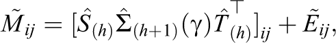
To fit the model with fixed effects, we adjust IFA to estimate these parameters in addition to the latent factors. Our steps are as follows: apply use sample averages to estimate μ.., μi., and μ.j with subtracting apply
Figure 8 shows the square root of the singular values of the IFA estimator, N*. The tuning parameter γ is chosen such that k = 3. This means that N* is a Rank 3 matrix, such that three latent factors contribute to the interaction outcome between the students and teachers in the school.
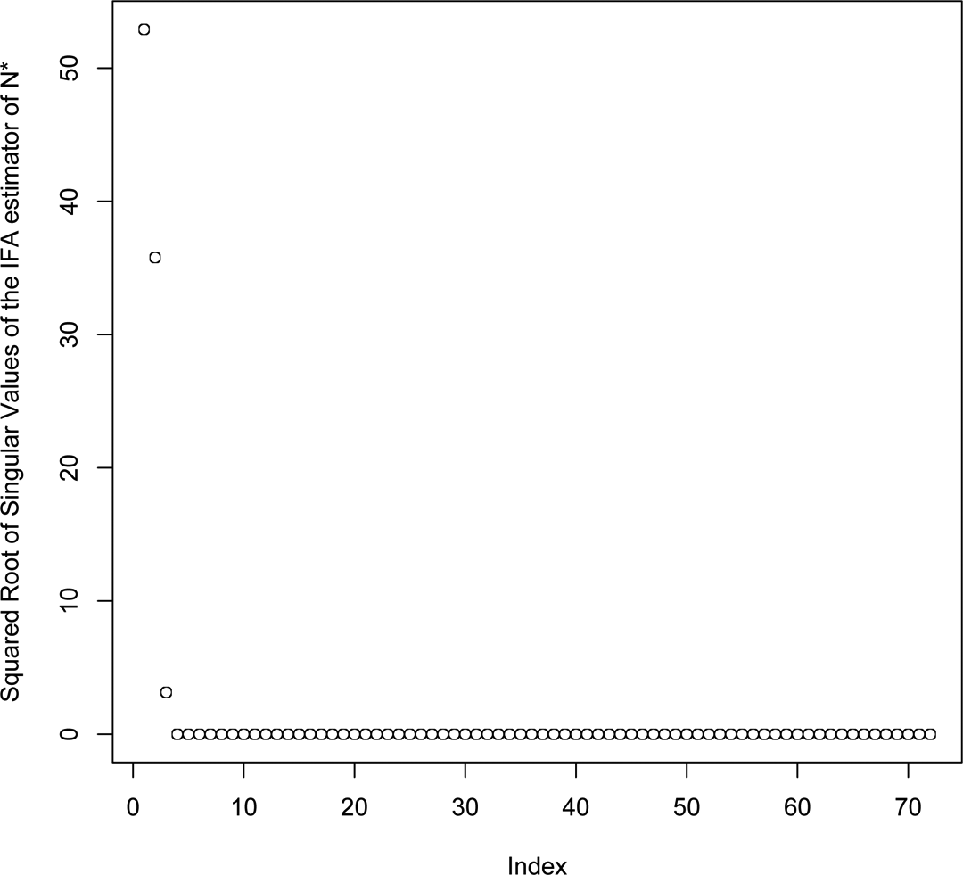
Square root of singular values of
Just as standard regression techniques will estimate parameters even if the true parameters are 0, IFA will still estimate an interaction even if none exists. That is, if the true process of student–teacher interactions is best approximated by a model with columns of S and T being 0 vectors in model (Equation 1), the IFA algorithm will still return estimates. The rest of this article uses a series of post hoc techniques to ensure that the results are statistically meaningful.
Post Hoc Analysis
Correlation Analysis Between Estimated Latent Student Factors and External Covariates
Suppose there is not any interaction effect between students and teachers; that S = 0 and T = 0. Under this null model, the estimates of S and T correspond to random noise and the first column of
There are seven
7
student-level measures in the institutional records, including whether the student is qualified for reduced-price lunch, homelessness status, race, gender, country of birth, primary language, and the primary language of the parents. Using each of these available measures as the response variable Y, we fit a logistic regression model using the three leading student latent factors from
p-Values of the Student Latent Factors When Being Used as the Covariates in the Linear Models

Note. Boldface values represent significant p-values (any value that is less than .1).
Regression results indicate the correlation between IFA-estimated student latent factors and several observed student-level measures, including whether the student qualifies for reduced-price lunch, homeless status, gender, and U.S.-born status. It is conceivable that student latent factors estimated by IFA do not need to correlate with the existing student variables, and instead, they may correspond to certain unmeasured student variables. Nevertheless, in this case, correlation between the latent factors and the existing student measures provides an external validation for the fact that IFA, applied to this school, detected an interaction effect between students and teachers. Importantly, the estimated latent factors
Whether a student qualifies for reduced-price lunch at school is a widely used proxy for his or her family SES (Caldas, 1993; Caldas & Bankston, 1997; Sirin, 2005). Regression results show that the relationships between latent student factors and the proxy for SES are statistically highly significant. This does not imply that high-SES students are at a particular advantage or disadvantage. Instead, it suggests that some teachers have positive interactions with high-SES students (and negative interactions with low-SES students), while other teachers have positive interactions with low-SES students (and negative interactions with high-SES students). Where an individual teacher falls on this spectrum is estimated in the corresponding teacher latent factor in
Table 1 shows that when one factor is significantly correlated, it is common for another to be correlated as well. Standard approaches from EFA, such as the VARIMAX rotation, could help to isolate these factors (Kaiser, 1959). The current post hoc analysis is used to establish a correlation between the estimated latent factors and the external covariates. In the future, we would like to take IFA to another step of developing a procedure that allows for interpretation of the individual meanings of the latent factors, given sufficient number of observed student and teacher covariates.
Similarly, the estimated teacher latent factors are correlated with two of the four teacher measures. The four measures that we were able to harvest are the average age of the students in the teacher’s class, race/ethnicity, number of years of experience, and the institution(s) of higher education from which he or she received credits. Each of those is fit into an appropriate linear model, and the average age of the students having exposed to the teacher along with the number of years of experience is correlated with our estimated teacher latent factors. Table 2 details the result.
p-Values of the Teacher Latent Factors When Being Used as the Covariates in the Linear Models

Note. Boldface values represent significant p-values (any value that is less than .1).
One possible concern is that the teacher latent factors in fact correspond to differential rates of growth in the students, that is, the students might perform better as they advance over the grades and the teacher latent factors estimate that effect. We believe this is not the case since the regression result does not indicate total correlation between the ages of the students in the teacher’s class and the teacher latent factor. Additionally, the FCAT score that we use, among many other student achievement measurements, is vertically scaled to adjust for this growth effect (McBride & Wise, 2000). The correlations between student latent factors and the external measurements on the students also indicate the relevance of
In a similar manner, one might worry about the change in preference of the students over the year. For example, gender preferences might be assortative for younger students, that is, the student and teacher pairs of the same gender have more positive interactions than those of opposite genders. Then, this gender effect becomes disassortative for older students, that is, the student and teacher pairs of opposite genders in turn have more positive interactions. This is a type of nonstationarity that IFA will be able to estimate in American schools. The key reason is that high school teachers do not have interactions with elementary school children. So, in this example, Si = 1 if i is a boy and Si = −1 if i is a girl. Then, Tj follows the same pattern if j teaches younger students, but an opposite pattern if j teaches older students. If teachers taught all levels of students, then this type of nonstationarity would not be detectable. For this reason, the assumed type of “stationarity” is that students of a similar type in Grade 3 also have a similar type in Grade 8. A potential direction for future research is to devise the statistical procedure to detect and remedy a violation of this stationarity assumption.
The Underlying Graph Structure
The assignment of students to teachers (i.e., the matrix B) is not random. It is chosen by the school. So, the elements of M* are not missing at random (MAR). A persistent source of bias in using regression techniques to study student–teacher interactions is the nonrandom assignment of students to teacher. In standard regression analysis, extending beyond MAR quickly becomes difficult and requires additional assumptions that are difficult to empirically validate. In a similar fashion, it is natural to suspect that the IFA estimates are confounded by the matrix B. If this is the case, it could introduce bias to the estimates.
Theoretical research by Foygel, Shamir, Srebro, and Salakhutdinov (2011) shows that the issue is not as severe for the matrix completion techniques studied in this article. In fact, a slight modification proposed by Foygel et al. allows for arbitrary sampling distributions that assign students to teachers. The next section examines this result with a simulation that retains the matrix B and creates measurements M* that correspond to a null model without interactions (i.e., S = 0 and T = 0).
Simulation to Validate that B Does Not Confound the Results
To further explore whether or not the interaction network affects the estimated singular values, we perform a simulation in which the student–teacher classroom assignment (i.e., B) is unchanged. Then the observed FCAT scores are replaced with random FCAT scores generated from a normal distribution with mean, variance, and cutoff points derived from the originally observed values in the interaction matrix M. We then apply IFA to the simulated matrix to derive its three leading singular values. Figures 9 and 10 show the distribution of those values over 100 simulations in cases where the fixed effects were included (matrix M*) and the fixed effects were removed (matrix N*), respectively. For the two leading singular values, the simulated values are significantly smaller than actual ones in both cases. In contrast, the third singular value is smaller than its corresponding simulated singular values. Since the regression results indicate its statistically significant correlation with the student’s qualification of reduced-price lunch, we decided to include it in our analysis. Regardless, this helps us confirm that, in fact, our observed latent factors are not dictated by the underlying graph structure. Instead, they provide us with meaningful signals about student–teacher interaction.
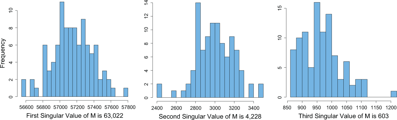
The histogram of the three leading simulated singular values of
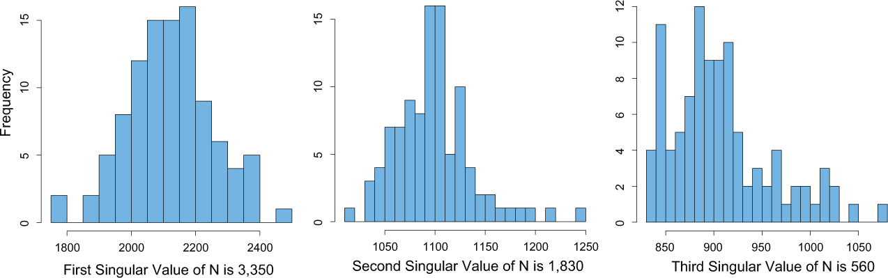
The histogram of the three leading simulated singular values of
Keeping the underlying bipartite graph structure intact, we also use these simulations to construct Tables 1 and 2. We regress each external measure on the simulated latent factors as we did in the Correlation Analysis section above and calculate the R2 for the linear regressions and pseudo R2. 9 The p-value is formulated as the portion of the (pseudo) R2 s achieved in the simulations that are greater than the (pseudo) R2 achieved using the actual data.
While the bias of IFA is largely insensitive to the sampling distribution of students to teachers, the student–teacher interaction network can increase the variability of IFA estimates if the network bifurcates into clusters of students and teachers that do not interact across the clusters. For example, if each student is assigned to a college track or a vocation track (and the teachers for these tracks do not overlap), then there are essentially two networks within one building. The IFA should only study one network at a time.
The analysis above studies grades kindergarten through eighth grade. Since it is more common to separate kids into different tracks in high school, it is not expected that this school separates into two tracks. Nonetheless, this can be confirmed by applying spectral clustering to the bipartite graph B. Using the spectral clustering techniques proposed by Qin and Rohe (2013), our investigation confirms that there is only a single network of students and teachers.
Robustness of the Signals
The previous results showed the estimated latent factors are related to external measures and that they are not confounded by the network structure in B. This section aims to understand how much error is in our estimates of the latent factors. Step 3 of IFA provides us with a low-rank estimator for M*,
where (1)
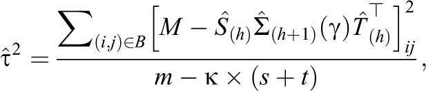
where m being the cardinality of set B or number of observed interactions between the students and teacher in M, m = 4,057, s = 1,276, t = 72, and k = 3 in this data set. Performing IFA on each simulated matrix
Cross-Validation
We have 4,057 observations of the student–teacher interaction observations to estimate 3 × 72 + 3 × 1,276 = 4,044 parameters. These parameters correspond to the three leading columns of S and T in Equation 1. Thus, IFA leaves us with only 13 degrees of freedom in this case. Given such a saturated model, we perform 405-fold cross-validation. In each fold, we randomly select 10 observations for validation, leaving out the other 4,047 observations for the training set. We apply IFA on this training set with the 10 chosen observations marked as missing. Our error rate is measured by the coefficient of variation of the root mean square error,
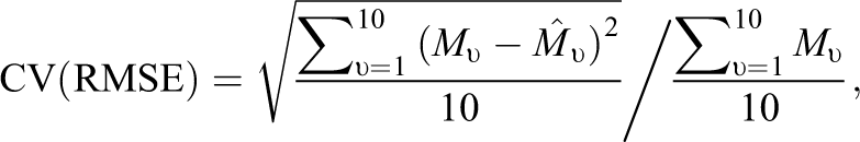
where Mυ are observed interactions used as validation,

Figure 11 illustrates the distribution of the error rates using results given by the three models. As we can see, adding latent factors as in IFA does improve the accuracy in estimating the student–teacher interaction outcomes compared to the models using only fixed effects.
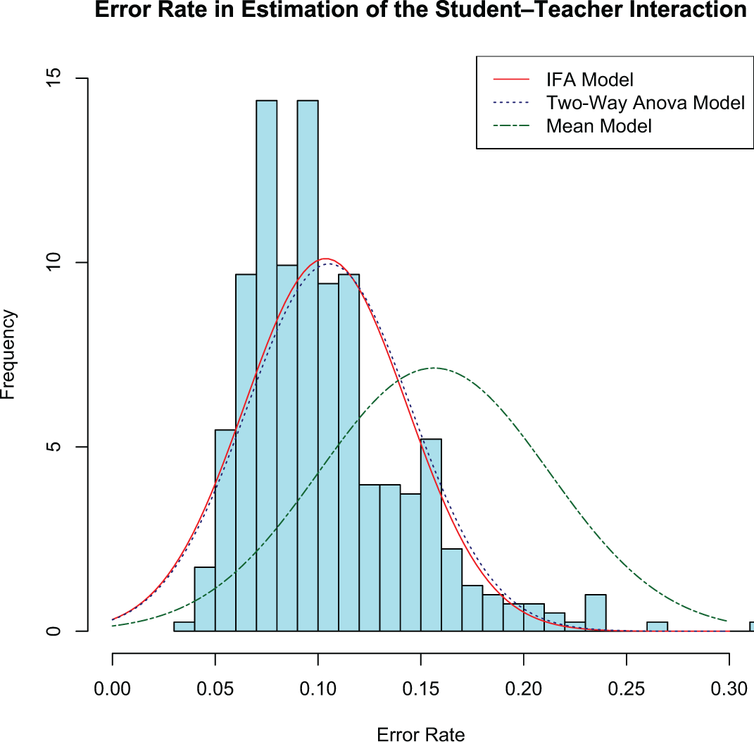
Accuracy measure over 405 folds of cross-validation. With only three degrees of freedom in estimating the missing observations, interaction factor analysis has an average error rate of 10%.
The Case of Student–Teacher Matching
The estimates of S and T are interesting in helping to interpret the interactions between students and teachers. They can also be used to predict the value of interaction between each student–teacher dyad. Such an application provides a path for recommending classroom assignments.
In the current application, we use the approach to examine the school’s classroom assignments. Specifically, we apply IFA on the original M matrix to fill in the missing FCAT scores. We plot the predicted score distribution in matrix
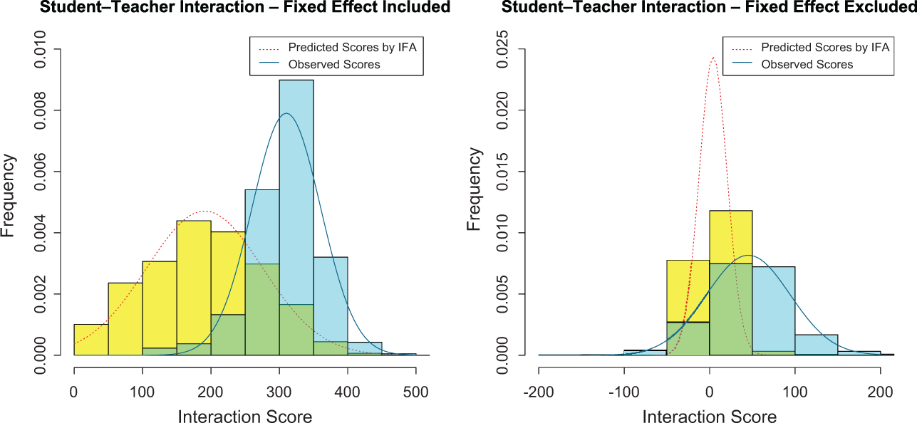
The left histogram shows the distributions of the observed and predicted student–teacher interactions before the fixed effects are remove. The right distributions of the observed and predicted student–teacher interactions after the fixed effects are removed. Both suggest that the school leaders may have insights about matching students and teachers.
Discussion
The field of education is in strong need of new tools that illuminate how teachers and students influence one another through the fundamental educational process of classroom interactions. IFA is a versatile exploratory tool that may help educational researchers understand the broad and underlying factors that underlie student–teacher interactions. IFA can be used to identify the types of student and teacher that work best together through prediction of the interactions. Thus, it provides a quantitative tool to help the school leaders in optimizing classroom assignment, given the pool of students and teachers.
The performance of IFA increases with the number of measured student–teacher interactions. At a minimum, if each student and each teacher has an average of three measured interactions, then IFA can estimate three latent factors. This was the case for the school studied in this article. If this number were to increase, the latent factor estimates would become less variable. In the current regime, the estimated latent factors
The techniques of IFA can be applied to any situation in which there are several interactions between two groups (e.g., students and teachers), and these interactions produce some quantity that measures their effectiveness. For example, IFA could be applied to studying the dynamics of the teacher labor market. Jackson (2013) applies linear mixed model in studying the mobility of teachers across the schools in the state of North Carolina. The research indicates that match quality between the teacher and the school goes beyond the teacher and school’s fixed effects. Certain types of teachers are more effective working in certain type of schools. We believe that IFA, when applied to studying this labor market, will compliment the findings. It will also help predict the outcome of the interaction between the teacher and the school.
In addition, the IFA approach is metric agnostic. In the Numerical Analysis section, we use state test scores because of the salience of the standardized exams in the United States. We can instead input the student–teacher interaction matrix M with any measures such as survey scores from the students or teachers, number of days the student absent in a semester, number of disciplinary actions taken by the teacher toward the students, number of positive interactions that the student and teacher share on average, Brophy–Good interaction system, or STRS. The interpretation of latent factors should be guided by choice of metric.
Applying IFA on M gives useful insights into the latent factors that drive the success of the student–teacher interactions. It also helps us answer the fundamental question of whether the student and teacher innate abilities alone can decide the outcome of the interaction or whether there are other factors that contribute to student success. Matching certain types of students to certain types of teachers can lead to more successful classroom interactions. Moreover, if future research can identify persistent latent factors, these could be used to coach teachers to adapt to student needs. In our illustration, we populated M with FCAT scores. This shows that interactions between students and teachers are quantifiable and multidimensional. In our belief, other measures could provide a more dimensional understanding of the student–teacher interactions. This will be an area for future research.
Admittedly, while our article focuses on the student–teacher interaction, the school is interwoven networks of interactions of many members. Aside from the student–teacher interaction one, we have peer-to-peer interaction network, student–principal interaction network, and student–parent interaction network. All of those factors can contribute to the student outcomes, and they are promising future research topics. There are two key advantages to focusing on the student–teacher interactions. First, every year, schools explicitly decide which students will interact with which teachers. As such, they have much more control over these interactions. Second, as a consequence of this control, there are several measurements that are already collected that provide some guidance on the quality of these interactions; in this article, we have focused on test scores. These advantages do not limit the importance of the other types of interactions but merely suggest a good place to begin these analyses.
Footnotes
Appendix A
Appendix B
Funding
The author(s) disclosed receipt of the following financial support for the research, authorship, and/or publication of this article: This research is supported by NSF grant DMS-1309998 and ARO grant W911NF-15-1-0423.