Rebar: Reinforcing a Matching Estimator With Predictions From High-Dimensional Covariates

Abstract

In causal matching designs, some control subjects are often left unmatched, and some covariates are often left unmodeled. This article introduces “rebar,” a method using high-dimensional modeling to incorporate these commonly discarded data without sacrificing the integrity of the matching design. After constructing a match, a researcher uses the unmatched control subjects—the remnant—to fit a machine learning model predicting control potential outcomes as a function of the full covariate matrix. The resulting predictions in the matched set are used to adjust the causal estimate to reduce confounding bias. We present theoretical results to justify the method’s bias-reducing properties as well as a simulation study that demonstrates them. Additionally, we illustrate the method in an evaluation of a school-level comprehensive educational reform program in Arizona.

Keywords

observational study causal inference matching machine learning

1. Introduction: Two Types of Neglected Data

Matching-based observational studies in education sciences often neglect data from the “remnant” of a match: untreated and unmatched subjects. That is, researchers will select a set of matched controls that most closely resemble the treated subjects and discard data from the remnant, the unmatched controls.

Similarly, due to sample size and other modeling limitations, researchers will typically condition their experimental and observational studies on a small set of pretreatment covariates that are deemed most relevant to the study—the variables thought most likely to pose a confounding threat. In many cases, reams of less relevant data are available, perhaps from state longitudinal data systems or from other sources. These less relevant covariates are often discarded.

Conducting a causal analysis using only the matched sample and using only relevant covariates makes good statistical sense. The data from subjects that are not part of a match are likely to be distributed differently than data from the match. The process of matching encourages researchers to focus their analysis on the region of common support; the remnant is typically outside this region by construction. Including irrelevant variables into an analysis can swamp the sample, introduce overfitting or extreme imprecision, and make impossible common statistical techniques such as ordinary least squares (OLS) and logistic regression.

But these excluded data—the remnant and ostensibly irrelevant covariates—may also contain valuable information. Perhaps the distribution of the outcome conditional on covariates could be estimated with more precision by vastly increasing the sample size using discarded subjects. Perhaps discarded covariates are not so irrelevant and capture important baseline differences between treated and untreated subjects.

This article is an attempt to thread this needle with a new method that we call “remnant-based residualization” or “rebar.” The idea of rebar is to, on the one hand, extract as much useful information as possible from the remnant and all available covariates and, on the other hand, to preserve the most attractive properties of a good matching design. To implement rebar, we fit a machine learning prediction model to the unmatched controls—the remnant—predicting their outcomes in the control condition as a function of the entire set of covariates. Using this fitted model, we then generate predicted outcomes for the matched sample. Finally, instead of calculating the effect of the treatment on participants’ outcomes themselves, we estimate the intervention’s effect on the difference between participants’ predicted outcomes under the control condition and their actual outcomes, that is, their prediction residuals—this is “residualization.” The predictive model need not be correct in any sense or consistent or unbiased for any particular parameter. It must only yield predictions that are closer, on average, to control potential outcomes than their mean.

Rebar builds thematically on prior work combining matching with outcome modeling, such as Rubin (1973) and Ho, Imai, King, and Stuart (2007a), among others, alongside “doubly robust” estimation (e.g., Kang & Schafer, 2007). Its most direct antecedents are Rosenbaum (2002a) and Abadie and Imbens (2012), which suggest forms of residualization for matching estimators, and Middleton and Aronow (2015), which does the same for weighting estimators. Our contribution to that literature is twofold: First, rebar is remnant-based. We argue here that residualization is well suited to recovering otherwise lost information from the remnant. Second, we demonstrate by simulation and example how rebar can exploit machine learning methods and high-dimensional covariates without compromising the classical statistical properties of the match.

Rebar can supplement a wide range of matching analyses and may be used alongside other outcome models and covariate adjustments.

The following section will review causal matching studies, and Section 3 will formally introduce rebar. There, we will discuss a possible threat to the validity of a matching design that rebar can introduce: If the distribution of outcomes, conditional on covariates, differs widely enough between the remnant and the matched set, rebar might increase, rather than decrease bias. We will introduce a diagnostic called “proximal validation” that should detect such pathological cases and suggest ways to tweak the algorithm if a researcher was to confront one.

Rebar can potentially reduce both the bias and the variance of causal estimates, by modeling otherwise unmodeled variation. That said, this article will focus its attention on rebar’s bias reducing properties. We will argue with analytical results (Section 4), a simulation study (Section 5), and an empirical example (Section 6) that rebar is an effective method for reducing confounding bias from measured, but unmodeled, confounders in a high-dimensional data set, without compromising the key advantages of matching.

2. Matching in Observational Studies: Review

In an observational study, let i = 1, …, n index n subjects, and let Z_i denote subject i’s binary treatment assignment, and Y_i subject i’s observed outcome of interest. Assuming noninterference (Cox, 1958) and following Neyman (1990) and Rubin (1974), let y_Ti and y_Ci denote subject i’s (perhaps counterfactual) responses were subject i treated and untreated, respectively. Then, $Y_{i} = y_{T i} Z_{i} + y_{C i} (1 - Z_{i})$ . Further, let x_i be a vector of covariates measured prior to treatment. The potential outcomes y_C and y_T define treatment effects τ_i = y_Ti − y_Ci and a causal estimand

τ_{E T T} = E_{Z} [τ^{T} Z / n_{T}] = \frac{τ^{T} E Z}{n_{T}},

the expected average effect of the treatment on the treated. The expectation in Equation 1 is taken conditional on the posited sampling scheme.

In a matching-based observational study, a researcher will create a new categorical variable, M , considering subjects i and j to be matched to one another if M_i = M_j. (Subjects i with the property that M_i ≠ M_j for all i≠j are unmatched.) Researchers will choose M in such a way that matched subjects have similar covariate distributions x. Perhaps the most popular approach to matching is to use propensity scores (Rosenbaum & Rubin, 1983), P_r(Z = 1|x), the probability of being assigned to treatment conditional on covariates x. In a propensity-score matching design, treated and untreated subjects are grouped into matches M with approximately equal estimated propensity scores. Other inexact matching techniques measure subjects’ similarity in x using, for example, Mahalanobis distances (Rubin, 1980) or covariate balance tests (Diamond & Sekhon, 2013). Matched sets may contain any (positive) number of treated or untreated subjects (Rosenbaum, 1991).

Ideally, within any matched set, no subject’s a priori probability of making its way into the treatment group was larger or smaller than any other’s:

P r (Z_{i} = 1 | M) = P r (Z_{j} = 1 | M) whenever M_{i} = M_{j},

this is perfect matching. Under perfect matching in the sense of Equation 2, matched comparisons are statistically equivalent to contrasts of treatment and control conditions in block- or paired-randomized designs (e.g., Braitman & Rosenbaum, 2002; Hansen, 2011; Rubin, 2008).

A simple matching-based estimator compares average treated and untreated outcomes within each match. The average difference between treated and untreated subjects in matched set m is:

t (Y_{m}, Z_{m}) = \frac{Y_{m}^{T} Z_{m}}{n_{T m}} - \frac{Y_{m}^{T} (1 - Z_{m})}{n_{C m}},

where Y_m and Z_m are the vectors of Y and Z, and n_Tm and n_Cm are the numbers of treated and untreated among subjects {i : M_i = m}. Then, a matching estimator is

{\hat{τ}}_{M} (Y) = \sum_{m} w_{m} t_{m} (Y, Z),

where weight w_m = n_Tm/n_T. Estimator ${\hat{τ}}_{M} (Y)$ is unbiased for τ_ETT under perfect matching (Equation 2), or, more generally, if the difference in assignment probabilities is uncorrelated with control potential outcomes (Lemma 1 in the Appendix). In practice, neither of these will be exactly true, but researchers can hope for approximate unbiasedness and explore their design’s sensitivity to unmeasured (or unmodeled) bias (e.g., Gastwirth, Krieger, & Rosenbaum, 1998; Hosman, Hansen, & Holland, 2010).

Frequently, subjects who are not sufficiently similar in x to other units are left unmatched. We will refer to the set of unmatched untreated subjects as the remnant from a match. Typically, the remnant is discarded. While discarding data might seem unwise, there is good reason to discard the remnant. Since no suitable comparisons may be found between subjects in the remnant and treated subjects, any causal comparisons using the remnant necessarily involve modeling y_C as a function of X . Moreover, the remnant typically occupies a mostly separate region of the distribution of X than the matched sample—hence its inability to be matched. Therefore, comparing outcomes from treated subjects with those from the remnant involves extrapolation, which can be highly sensitive to model specification. On the other hand, the remnant may contain information that is useful for modeling y_C.

An extensive, occasionally contentious literature discusses variable selection for propensity score models. This literature begins with Rubin and Thomas, who advised erring on the side of inclusiveness, striving to exclude only those covariates that a consensus of researchers believe to be unrelated to each outcome variable (1996, §2.3); Rosenbaum’s (2002b, p. 76) view is similar. Later contributions argued that including variables only weakly related to outcomes may increase the mean-squared error (MSE) of effect estimation (Austin, 2011; Brookhart et al., 2006). These additional losses can in principle take the form of bias, not only variance, even if the MSE-increasing variable was determined in advance of treatment assignment (Greenland, 2003; Pearl, 2009; Sjölander, 2009). Most recently, Steiner, Cook, Li, and Clark (2015) argued via case study for including all available covariates, unless “strong substantive theory” (p. 573) suggests the presence of bias-amplifying covariates covariates (they write that bias amplification “seems less likely as the size of the covariate set increases”); ideally, researchers should include covariates from multiple domains, with each domain including as many covariates as possible. Pimentel, Small, and Rosenbaum (2016) suggested conducting two analyses, each matching on a different set of covariates. Methods attempting to limit the MSE penalty by limiting propensity modeling variables to those that correlate with observed outcomes have been met with criticism of a different nature: In Rubin’s view, in order to maximize objectivity, during matching researchers should keep outcome measurements in a virtual locked box, only to emerge once the matching structure and other study design elements have been determined (Rubin, 2008).

Rebar, the method of this article, is compatible with either attitude to selection of propensity score variables; our illustration (§6) emphasizes this compatibility by adhering to the more restrictive of the two schools. Without reference to outcome associations, we select for inclusion in the propensity model those variables we felt that a consensus of scholars would be most likely to deem potential confounders. In this example as in many others, the number of potential confounders that could be addressed in this way was limited: When p ≥ n_T or p ≥ n_C, then the treatment and control samples can ordinarily be separated by a hyperplane, in the space spanned by X , with the result that common binary regression methods fail to fit (Agresti, 2013; Zorn, 2005); in the example of §6, n_T = 7. This heightens the need for additional measures for confounder control, such as rebar.

3. Rebar: Using an Outcome Model to Reduce Bias in a Matching Design

The procedure we recommend is the following:

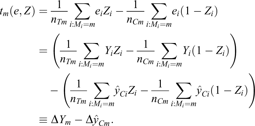
Using the full data set, construct a match M , perhaps based on a subset of available covariates, thereby dividing the sample into a matched sample and a remnant.

Using units in the remnant, construct an algorithm ${\hat{y}}_{C} (\cdot)$ to predict y_C as a function of the full matrix X .

Assess the performance of ${\hat{y}}_{C} (\cdot)$ (see Section 3.1).

For all subjects i in the matched sample, use ${\hat{y}}_{C} (\cdot)$ to predict y_Ci as ${\hat{y}}_{C i} = {\hat{y}}_{C} (x_{i})$ .

Construct prediction errors $e \equiv Y - {\hat{y}}_{C} (X)$ for all subjects in the matched sample.

Estimate treatment effects in the matched sample, substituting e for Y in the outcome analysis.

As in Rosenbaum (2002a), the model ${\hat{y}}_{C} (\cdot)$ relating X and y_C is an algorithmic model, rather than a statistical model. That is, it does not estimate parameters of a probability distribution, but rather generates deterministic predictions of y_C when given a vector x. Since this procedure relies on the residuals of a model fit to Y, we will refer to it as residualization.

The predictions ${\hat{y}}_{C} (x)$ bear some similarity to prognostic scores (Hansen, 2008). Prognostic scores, which are analogous to propensity scores, are statistics that are sufficient for the relationship between y_C and x. They are commonly understood as predictions of y_C as a function of x (e.g., Pane, Griffin, McCaffrey, & Karam, 2013). In fact, much of the intuition behind prognostic scores supports our use of ${\hat{y}}_{C} (x)$ here, though the prognostic score theory will not play a direct role in our argument.

Now, as above, define residuals,

e = Y - {\hat{y}}_{C} (x) .

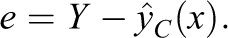
Then, we may define “potential residuals”: $e_{C} = y_{C} - {\hat{y}}_{C} (x)$ and $e_{T} = y_{T} - {\hat{y}}_{C} (x)$ . Analogously to Y, the observed residuals are $e = Z e_{T} + (1 - Z) e_{C}$ . Crucially,

e_{T i} - e_{C i} = τ_{i},

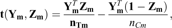
where τ_i as above is subject i’s treatment effect, y_Ti − y_Ci. To see this, note that $y_{C} = {\hat{y}}_{C} (X) + e_{C}$ and $y_{T} = {\hat{y}}_{C} (X) + e_{T} = {\hat{y}}_{C} (X) + e_{C} + τ$ . The prediction ${\hat{y}}_{C} (x)$ is based only on pretreatment variables x and not on treatment status Z from subjects in the matched sample. That being the case, it cannot be affected by treatment status—we would counterfactually estimate the same ${\hat{y}}_{C} (x)$ for alternative realizations of Z in the matched set. Therefore, we can write $e_{T i} - e_{C i} = y_{T i} - {\hat{y}}_{C i} - (y_{T i} - {\hat{y}}_{C i}) = y_{T i} - y_{C i} = τ_{i}$ : The treatment effect is manifest entirely in the residuals e_C and e_T, and not at all in ${\hat{y}}_{C} (x)$ .

The prediction errors e, then, may replace Y in an outcome analysis. In particular, replace matched-set-specific treatment-control differences in Y, t_m(Y,Z) with differences in e: t_m(e,Z). That is, let

t_{m} (e, Z) = {\bar{e}}_{m, Z = 1} - {\bar{e}}_{m, Z = 0} = \frac{1}{n_{T m}} \sum_{i : M_{i} = m} e_{i} Z_{i} - \frac{1}{n_{C m}} \sum_{i : M_{i} = m} e_{i} (1 - Z_{i}),

then define

{\hat{τ}}_{rebar} = \sum_{m} w_{m} t_{m} (e, Z) .

Residualization, then, means revising a matching estimator by replacing outcomes y with observed value/ ${\hat{y}}_{C} (\cdot)$ differences; it aims to rid the dependent variable of variation that is not informative about treatment effects. Rosenbaum (2002a) precedes conventional hypothesis tests with a residualization step, using observations within the matched sample to fit the prediction model. If one instead trains one’s prediction algorithm ${\hat{y}}_{C} (\cdot)$ using the remnant of the matching procedure, the method becomes compatible with common estimation (as well as hypothesis testing) techniques and may offer larger numbers of observations for training ${\hat{y}}_{C} (\cdot)$ . Such remnant-based residualization, briefly rebar, is the topic of this article.

3.1. Cross-Validation and Proximal Validation: Assessing ${\hat{y}}_{C} (\cdot)$

Using the remnant to model outcomes as a function of covariates affords the researcher a great deal of flexibility. Researchers may use data from the remnant—both covariates and outcomes—to attempt a variety of prediction techniques and choose the one which performs best. This is particularly important when the dimension of X is large, so formulating statistical models based on theory or first principles is hard or impossible; a variety of methods must be attempted. A useful tool in this regard is k-fold cross-validation (Efron & Gong, 1983), which can estimate the predictive accuracy of a model using data from the training sample. Cross-validation results may be examined for bias, variance, or other measures of predictive performance, but Proposition 3 (below) suggests a focus on prediction MSE. In the rebar case, cross-validation using data from the remnant can estimate ${MSE}_{remnant} = E_{i \in remnant} {({\hat{y}}_{C i} - y_{C i})}^{2}$ or $R_{remnant}^{2} = 1 - {MSE}_{remnant} / {Var}_{remnant} (y_{C})$ .¹ These results can be used both to pick a modeling technique and to pick tuning parameters. After modeling choices have been made, researchers arrive at an estimated prediction function ${\hat{y}}_{C} (\cdot) : ℝ^{p} \to ℝ$ that generates predictions ${\hat{y}}_{C} (X)$ as a function of covariates X .

Cross-validation estimates an algorithm’s predictive performance when applied to new cases drawn from the same population as the training set. Of course, this is manifestly not the case for rebar. Subjects in the matched sample are likely to be different from those in the remnant; a model fit and cross-validated in the remnant may not perform as well in the matched sample as that validation would suggest. Write S_M to denote the matched sample, that is, ${i : \exists j \neq i s.t. M_{i} = M_{j}}$ . One expects MSE_remnant to be less than ${MSE}_{M} = {\sum_{i \in S_{M}} {({\hat{y}}_{C i} - y_{C i})}^{2}} / | S_{M} |$ , and $R_{remnant}^{2}$ to be less than $R_{M}^{2}$ . This is unfortunate but far from fatal—the more information a prediction algorithm can learn about the matched sample from the remnant, the better rebar can reinforce a causal design. Perfection is not necessary.

One does not expect MSE_M to exceed ${\sum_{i \in S_{M}} {(y_{C i} - {\bar{y_{C}}}_{S_{M}})}^{2}} / | S_{M} |$ , although this can occur. In such cases, rebar could do more harm than good. Even with perfect matching in the sense of Equation 2, it could diminish efficiency, and if Equation 2 is only approximately true, rebar could increase bias as well.

Fortunately, simple diagnostic tools can identify such pathological cases. Further, in many of those cases, there are simple modifications to rebar that will improve its performance. To illustrate a diagnostic that we call proximal validation, consider full matching within calipers of width c₀ in terms of a continuous variable or index, such as the propensity score. All control subjects within c₀ of a treated subject are matched, with remaining controls constituting the remnant. How well does an algorithm ${\hat{y}}_{C} (\cdot)$ fit in the remnant perform in the matched sample? To gauge ${\hat{y}}_{C} (\cdot)$ ’s performance, a researcher will subdivide the remnant into two groups by using caliper c₁ > c₀ to construct a new, larger matched set. The cases in the remnant that are matched under with the more permissive caliper c₁ are “proximal” cases—whether they are matched depends on the choice of caliper. The cases that remain unmatched even under c₁ are “distal” cases, unmatchable under either scheme. Proximal validation refits ${\hat{y}}_{C} (\cdot)$ using only data from subjects in the distal remnant, then examines its performance on the proximal portion of the remnant. If ${\hat{y}}_{C} (\cdot)$ performs poorly when extrapolated from the remnant to the matched set, it likely also performs poorly when extrapolated from distal cases to proximal cases within the remnant. In other words, proximal validation is a way to gauge the performance of ${\hat{y}}_{C} (\cdot)$ when its results are extrapolated in a way analogous to a matching design.

As compared to estimating MSE_M with rebar’s MSE on the control group, proximal validation permits the analyst to keep matched subjects’ outcomes in Rubin’s (2008) virtual locked box, even as the rebar model is being validated and improved. Proximal validation is not limited to propensity-score full-matching designs with calipers; it may be used with any matching design that involves a quantitative restriction on allowable matches. The procedure, in general, will be to slightly relax that restriction, choose a second, more expansive match, and use the results to divide the remnant into proximal and distal portions.

If ${\hat{y}}_{C} (\cdot)$ ’s performance in proximal validation is discernibly worse than its cross-validation performance, the rebar routine should be modified. Suppose the mechanism selecting untreated units between the remnant and the matched sample is matching based on an estimated propensity score. In this case, the estimated propensity score itself can be incorporated into the prediction model ${\hat{y}}_{C} (\cdot)$ —for instance, by including interaction terms between the columns of X and $\hat{π}$ .

Another useful diagnostic test is to check covariate balance on the predictions ${\hat{y}}_{C} (X)$ . Since ${\hat{y}}_{C} (X)$ is a covariate, a successful matching design will ensure that its distributions are similar among treated and matched untreated subjects. Even though ${\hat{y}}_{C} (X)$ is a constructed variable, because the model behind it is fit without reference to the matched sample, balance on it can be tested in the same ways balance on manifest variables can be tested. If a balance test rejects the hypothesis of ${\hat{y}}_{C} (X)$ balance, researchers may revise either the prediction algorithm ${\hat{y}}_{C} (\cdot)$ , the matching scheme, or both.

4. Rebar’s Effects on Bias

To see the potential of rebar to reduce the bias of a matching estimator, note that the rebar estimator ${\hat{τ}}_{rebar}$ can be expressed as the difference in two estimated treatment effects:

{\hat{τ}}_{rebar} = {\hat{τ}}_{M} (Y) - {\hat{τ}}_{M} ({\hat{y}}_{C}),

the matching estimator of the effect of the treatment on Y, minus an estimate of the effect of the treatment on ${\hat{y}}_{C} (X)$ . To see this, note that

t_{m} (e, Z) = \frac{1}{n_{T m}} \sum_{i : M_{i} = m} e_{i} Z_{i} - \frac{1}{n_{C m}} \sum_{i : M_{i} = m} e_{i} (1 - Z_{i}) = (\frac{1}{n_{T m}} \sum_{i : M_{i} = m} Y_{i} Z_{i} - \frac{1}{n_{C m}} \sum_{i : M_{i} = m} Y_{i} (1 - Z_{i})) - (\frac{1}{n_{T m}} \sum_{i : M_{i} = m} {\hat{y}}_{C i} Z_{i} - \frac{1}{n_{C m}} \sum_{i : M_{i} = m} {\hat{y}}_{C i} (1 - Z_{i})) \equiv Δ Y_{m} - Δ {\hat{y}}_{C m} .

The expression in Equation 6 follows by taking weighted averages of ΔY_m and $Δ {\hat{y}}_{C m}$ . Of course, the treatment cannot have an effect on ${\hat{y}}_{C} (X)$ , which is a function of pretreatment covariates and a separate sample; any observed “effect” of the treatment on ${\hat{y}}_{C} (X)$ must be the result of covariate imbalance.

Two properties of the rebar estimate follow immediately. First,

Proposition 1:

bias ({\hat{τ}}_{rebar}) = bias ({\hat{τ}}_{M} (Y)) - {\hat{τ}}_{M} ({\hat{y}}_{C}) .

Viewing ${\hat{τ}}_{M} ({\hat{y}}_{C})$ as an estimate of ${\hat{τ}}_{rebar}$ ’s bias, the effect of residualization is to subtract from the matching estimator an estimate of its bias. (As with other bias correction methods, it backfires when the bias is poorly estimated, an eventuality proximal validation aims to detect.)

Next,

Proposition 2: Under perfect matching (2), ${\hat{τ}}_{rebar}$ is unbiased for τ_ETT.

This follows since, when treatment is essentially randomized within matches, $E {\hat{τ}}_{M} (Y) = τ_{ETT}$ and $E {\hat{τ}}_{M} ({\hat{y}}_{C}) = 0$ . So in a successful matching design, rebar does not introduce bias. Propositions 1 and 2 hold for any effect estimator $\hat{τ} (\cdot)$ that is linear in outcomes Y, that is, for which Equation 6 holds.

4.1. An Upper Bound on the Bias of the Rebar Estimator

The closer, on average, predictions $\hat{y} (x)$ are to control potential outcomes in the matched set, the smaller the bias of ${\hat{τ}}_{rebar}$ must be.

Proposition 3: In a matching design, the squared bias of ${\hat{τ}}_{rebar}$ can be bounded as

{bias (\hat{τ}}_{rebar})^{2} \leq {MSE}_{M} \times C (n, n_{T}, n_{C}),

where ${MSE}_{M} = \sum_{i \in matched} {({\hat{y}}_{C i} - y_{C i})}^{2} / n_{M}$ , n_M is the number of subjects in the matched set, and

C (n, n_{T}, n_{C}) = \frac{n}{n_{T}^{2}} \sum_{m} (n_{C m} + n_{T m}) max {(1, \frac{n_{T m}}{n_{C m}})}^{2} .

Equivalently,

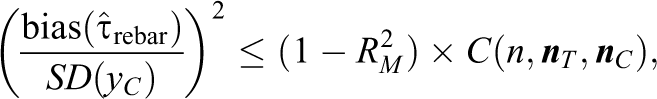
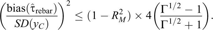
{(\frac{bias ({\hat{τ}}_{rebar})}{SD (y_{C})})}^{2} \leq (1 - R_{M}^{2}) \times C (n, n_{T}, n_{C}),

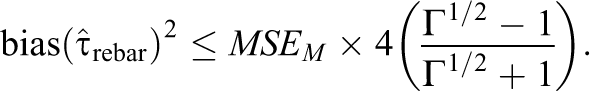
where SD(y_C) is the sample standard deviation of y_C in the matched set and $R_{M}^{2}$ is the prediction R² in the matched set, $1 - \sum_{i \in matched} {(y_{C i} - {\hat{y}}_{C i})}^{2} / \sum_{i \in matched} {(y_{C i} - {\bar{y}}_{C matched})}^{2}$ . (The proof can be found in the Appendix.)

Remark 1: In a pair-matching design $C (n, n_{T}, n_{C}) = 4$ .

Therefore, the bias of ${\hat{τ}}_{rebar}$ can be bounded as a function of the average squared error of the prediction algorithm in the matched set. Were it possible to perfectly predict all subjects’ y_C values, their treatment effects could be estimated unbiasedly (exactly, in fact). More broadly, Proposition 3 suggests that prediction algorithms need not be based on a correct model to yield estimates with low bias. They must merely be accurate, on average. This, in turn, suggests that machine learning algorithms, whose central purpose tends to be prediction, can serve well as residualization mechanisms.

In practice, the bounds in Proposition 3 are unobservable, since they involve control potential outcomes in the matched set, which are only observable for the matched controls. Further, since the prediction algorithm ${\hat{y}}_{C} (\cdot)$ is fit in the remnant, the bounds are not directly estimable without strong assumptions. But based on cross-validation estimates of MSE_remnant and $R_{remnant}^{2}$ , and an assessment of ${\hat{y}}_{C} (\cdot)$ ’s sensitivity to extrapolation from proximal validation, researchers can formulate reasonable guesses as to the values of MSE_M and $R_{M}^{2}$ .

Proposition 3 assumed nothing about subjects’ respective probabilities of treatment assignment within matches. In particular, it allowed for a situation in which some subjects may be assigned to treatment with probability 1—this is a rather extreme violation of the stratified randomization assumption (Equation 2). Under weak assumptions about the distribution of treatment assignments, the bound in Proposition 3 may be considerably tightened. For instance, Rosenbaum (2002b) suggests a general model for sensitivity analysis for observational studies: the assumption that for some Γ ≥ 1, if M_i = M_j—that is, i and j are in the same matched set—and P_i = P_r(Z_i = 1) and P_j = P_r(Z_j = 1), then

\frac{1}{Γ} \leq \frac{P_{i} (1 - P_{j})}{P_{j} (1 - P_{i})} \leq Γ .

That is, for matched subjects i and j, the ratio of the odds that i is selected for treatment to the odds that j is selected is bounded by 1/Γ and Γ. Proposition 4 uses the framework in Equation 7 to tighten the bound in Proposition 3 in the simple case of a matched-pair design; an analogous result may hold for more complex designs, but we leave such an extension for future work.

Proposition 4: In a pair-matching design, if Equation 7 holds for some Γ ≥ 1, then

{bias (\hat{τ}}_{rebar})^{2} \leq {MSE}_{M} \times 4 (\frac{Γ^{1 / 2} - 1}{Γ^{1 / 2} + 1}) .

Equivalently,

{(\frac{{bias (\hat{τ}}_{rebar})}{SD (y_{C})})}^{2} \leq (1 - R_{M}^{2}) \times 4 (\frac{Γ^{1 / 2} - 1}{Γ^{1 / 2} + 1}) .

(The proof may be found in the Appendix.)

Remark 2: For Γ = 6, which Rosenbaum (2002b, p. 114) characterized as “a high degree of insensitivity to hidden bias,” $4 (\frac{Γ^{1 / 2} - 1}{Γ^{1 / 2} + 1}) \approx 1.7.$ That is, a very weak assumption about the balance of treatment assignment probabilities in a matched pair design constricts the bound in Proposition 3 by more than half. If Γ = 3, the multiplier on $(1 - R_{M}^{2})$ is approximately one. On the other hand, as Γ → ∞, the multiplier approaches 4, as in Remark 1.

Propositions 3 and 4 show that by using data from the remnant and covariate matrix X to predict potential outcomes y_C, researchers can substantially bound the bias of their treatment effect estimates. The closer the estimates are to the true values, on average, the lower the bound on the bias—the algorithm ${\hat{y}}_{C} (\cdot)$ need not be correct in any sense, only predictive.

5. A Simulation Study

This section presents a simulation study with two principal goals: to demonstrate rebar’s potential to improve upon matching estimators under a variety of circumstances, and rebar’s ability to interact with, and improve upon, a variety of matching designs and estimators. A second, smaller study examines rebar’s performance under pathological circumstances.

5.1. Data-Generating Models

The study imagined a researcher estimating the effect of a treatment Z on an outcome Y, using a sample of n = 400 subjects, in the presence of p = 600 covariates. While all of the covariates are potential confounders, the simulated researcher knows that five of the covariates—the first five columns of covariate matrix X —predict both y_C and Z; prior background knowledge provides little guidance regarding the remaining 595.

The outcomes y_C were generated as a linear function of a multivariate normal vector X_i:

y_{C i} = 1^{T} x_{i, 1 : 5} + β^{T} x_{i, 6 : 600} + ϵ_{i},

where the coefficients β were drawn from an exponential distribution with a rate of λ = 5 and ϵ is drawn from a standard normal distribution. A “treated” group was selected according to probabilities

P r (Z_{i} = 1 | x_{i}) = {logit}^{- 1} (α^{*} + 1^{T} x_{i, 1 : 5} + {κβ}^{T} x_{i, 6 : 600}) .

That is, the log odds of treatment assignment were linear in covariates. We chose the parameter α* in such a way that, on average, n_T = 50 were treated. As in Equation 8, the coefficients for the first five columns of X in Equation 9 were all set equal to 1. The coefficients of the other 595 columns in Equation 9 were the same as in Equation 8, multiplied by a factor κ which varied between simulation runs.

The factor κ controlled the amount of confounding after matching. When κ = 0, only the first five columns of X predict Z, so estimates from a match based on those covariates should be approximately unconfounded. When κ > 0, every column of X predicts both Z and y_C, and therefore confounds matching estimators that use only the first five columns of X . As κ increases, so does the magnitude of the bias due to confounding after the match; the three values we assigned, κ = 0, .1, .5, roughly correspond to zero, low, and high unmatched confounding.

A second parameter, ρ, controlled the covariance structure of X , effectively controlling the ease of predicting y_C as a function of X . In this simulation, ρ = 0, .004, and .05. The rows of X were generated from a p = 600-dimensional multivariate normal distribution, with a random covariance matrix whose eigenvalues we specified (it was generated with R code of Varadhan [2008]). We set these eigenvalues ev_k, k = 1, ..., 600, to decay exponentially: ev_k = exp{−ρk}. When ρ = 0, all eigenvalues were unity, and the columns of X are uncorrelated. As ρ increases, the columns of X became increasingly correlated: There is low-dimensional structure in X . Prediction algorithms typically perform better when high-dimensional X can be summarized with a low-dimensional structure. During the simulation, we recorded the estimated prediction R² from the cross-validation, and models fit to X with higher ρ fit substantially better.

Covariates X and coefficients β varied between scenarios (one random matrix x for each value of ρ and one random vector β for each value of κ) but were held fixed across simulation runs within scenarios. Outcomes Y and treatment assignments Z were generated anew in each simulation run. Each run, all 10 effect estimates were computed using the same data.

5.2. Treatment-Effect Estimators

In each round of the simulation, we constructed four matches. Each of these matches, in turn, gave rise to two or three treatment-effect estimates; all in all, we compared 10 different estimators. These are summarized in Table 1.

Table 1.

Summary of the Matching and Estimation Methods in the Simulation Study

Matching Method	Propensity Score Model	Matching Variables	Adjustment Method(s)
Optimal pair match	Logit	X _1:5	Rebar
Nearest neighbor	Logit	X _1:5	Bias adjusted
Nearest neighbor	Logit	X _1:5	Bias adjusted + rebar
Coarsened exact match	N/A	X _1:5	Within-sample OLS
Coarsened exact match	N/A	X _1:5	Within-sample OLS + rebar
Optimal pair match	SuperLearner	X	Rebar

Note. X is a matrix of simulated covariates; subscripts denote selected columns. OLS = ordinary least squares.

Optimal pair matching with propensity scores from logistic regression

We estimated propensity scores using logistic regression, with Z regressed on the matching covariates, the first five columns of X . Using these propensity scores, we constructed an optimal pair match without replacement—each treated subject was matched to a unique control subject in such a way that the total distance in propensity scores between matched subjects was minimized. (We used the optmatch package in R [Hansen & Klopfer, 2006] and chose pair matching strictly for ease of interpretation; the application of §6 uses optmatch to pair each treatment group member to 1–4 controls.) We first estimated treatment effects via Equation 3, the average difference in Y between treated subjects and their matched controls, without adjustment from an outcome model.

Next, we computed rebar-adjusted estimates. With the remnant from the pair match as a training set, we used a combination of lasso (Tibshirani, 1996) and random forests (Breiman, 2001) to construct ${\hat{y}}_{C} (\cdot)$ , a predictor of control potential outcomes y_C as a function of the entire covariate matrix X . We implemented these in R with the glmnet and randomForest packages (Friedman, Hastie, & Tibshirani, 2010; Liaw & Wiener, 2002) and tuned and combined them with SuperLearner package (Polley & van der Laan, 2014) to minimize MSE. As outlined in Section 3, we used the fitted ${\hat{y}}_{C} (\cdot)$ to construct predictions ${\hat{y}}_{C}$ and prediction errors e in the matched set and estimated the treatment effect as in Equation 5.

Nearest-neighbor match with propensity scores from logistic regression

Using the same propensity scores as in the optimal pair match, we constructed a “nearest-neighbor” match, as proposed by Abadie and Imbens (2006), and implemented by the Matching package in R (Sekhon, 2011). We used the “ATT” estimator of Abadie and Imbens (2006) to estimate the average of the differences between each treated subject’s outcome and the average outcome of its matched controls. Next, we computed the “bias-adjusted” estimator suggested in Abadie and Imbens (2012), using an OLS outcome model fit to the matched sample.² Since OLS cannot be fit when the number of covariates exceeds the sample size, we used only the matching covariates for the bias adjustment. Finally, we combined within-sample bias adjustment with rebar. As in optimal pair matching, we fit the lasso/random forest/SuperLearner algorithm to data from the remnant from the nearest-neighbor match, predicting y_C as a function of the entire matrix X , and computed ${\hat{y}}_{C}$ and e in the matched set. To estimate effects with both within-sample and rebar adjustment, we substituted e for Y in the bias-adjusted estimator.

Coarsened exact matching

We constructed a coarsened exact match, as described in Iacus, King, and Porro (2011) and implemented in R with the cem package (Iacus, King, & Porro, 2015). We coarsened each of the first five columns of X with five bins, matched exactly on the coarsened covariates, and estimated treatment effects via Equation 3. Next, we constructed a within-sample-adjusted estimator along the lines of Ho, Imai, King, and Stuart (2007b): Using only data from the matched sample, we regressed Y on Z and the first five columns of X and recorded the coefficient on Z. Finally, we combined the within-sample adjustment with rebar. As in the optimal pair and nearest neighbor analyses, we used data from the remnant to fit a lasso/random forest/SuperLearner algorithm predicting y_C as a function of the entire X and generated predictions ${\hat{y}}_{C}$ and errors e in the matched set. To estimate effects, we regressed e on Z and the first five columns of X and recorded the coefficient for Z.

Optimal pair matching with propensity scores from SuperLearner

The first three matching designs, optimal pair matching, nearest-neighbor matching, and coarsened exact matching, used only the first five columns of X —the known confounders. However, when presented with a set of p = 600 covariates, many real-world researchers would not stop at the first five. Instead, they would try to incorporate additional covariates into their matches. The resulting iterative process of matching and balance checking is difficult or impossible to simulate; however, there are a number of automatic machine learning algorithms for estimating probabilities in high-dimensional spaces (e.g., Lee, Lessler, & Stuart, 2010; McCaffrey et al., 2013). In this vein, in parallel to the rebar prediction model ${\hat{y}}_{C} (\cdot)$ , we estimated high-dimensional propensity scores with random forest classification and lasso logistic regression, tuned and combined via the SuperLearner. We used these high-dimensional propensity scores to construct a second optimal pair match. As in the conventional pair match, we estimated effects using Equation 3 and, fitting algorithm ${\hat{y}}_{C} (\cdot)$ to the remnant, we computed a rebar estimate.

5.3. Simulation Results

Figure 1 shows the results of the simulation, after 1,000 simulation runs. Each row of Figure 1 corresponds to a value of κ; in the first row, κ = 0, corresponding to approximately no confounding from the covariates not used in the match, in the second row κ = .1, corresponding to moderate confounding from the left-out covariates, and in the third row κ = .5, corresponding to a high degree of confounding. Each column of Figure 1 corresponds to a different value of ρ: 0, .004, and .05. 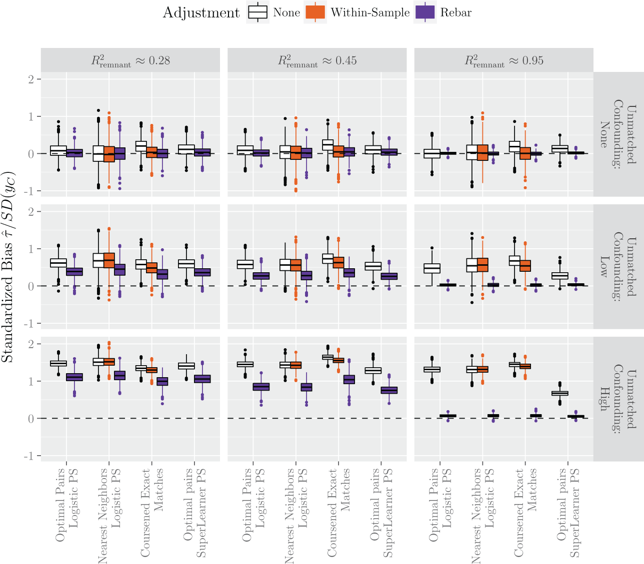These correspond to data sets increasingly amenable to prediction algorithms; the top of the figure lists the average cross-validation $R_{remnant}^{2}$ of ${\hat{y}}_{C} (\cdot)$ fit in the remnant from the pair match in the κ = 0 case (R² values for other models and other values for κ were similar). Each panel of Figure 1 displays boxplots of the 10 treatment effect estimates, divided by the standard deviation of y_C.

Figure 1.

Boxplots of treatment effect estimates from 1,000 simulation runs under the data-generating models in Section 5.1. The true treatment effect of zero is indicated by a horizontal dotted line. The estimated treatment effects were divided by the standard deviation of y_C. The matching and outcome adjustment methods are described in Section 5.2 and Table 1. The nine simulation scenarios, described in Section 5.1, are arranged in a matrix, with rows for κ = 0, .1, and .5, and columns for ρ = 0, .004, and .05. The $R_{remnant}^{2}$ values listed are averages of prediction R² for ${\hat{y}}_{C} (\cdot)$ estimated using cross-validation within the remnant.

A number of patterns are apparent. When κ = 0, the covariates not used in the match do not pose a confounding threat, and all the estimators are unbiased. Both within-sample bias reduction and rebar reduce the variance of the effect estimates, subtly for the first two columns and dramatically in the third. As κ, or confounding from the nonmatching covariates, increases, all effect estimates become increasingly biased. However, rebar substantially reduces the bias. Rebar is similarly effective when used on its own and when used in conjunction with within-sample outcome model adjustments—that is, rebar has quite a bit to add even after other adjustments. Unsurprisingly, rebar’s performance, both in terms of bias and variance reduction, improves with higher $R_{remnant}^{2}$ —the closer, on average, the predictions ${\hat{y}}_{C} (X)$ are to y_C in the remnant (and, presumably, in the matched set, too), the more good rebar can do.

The high-dimensional propensity score match demonstrates that rebar can improve upon designs that incorporate all of X .

This simulation study showed rebar’s potential: Rebar can substantially reduce both the bias and the variance of a matching estimator, especially in the presence of high-dimensional confounding and with an accurate prediction algorithm.

5.4. Rebar’s Performance Under Nonlinearity

We conducted a parallel simulation study to investigate rebar’s performance when the distribution of y_C, conditional on X, differs greatly between the remnant and the matched set. Since it is the match that determines which subjects are in the matched set and which are in the remnant, and the data generation occurs prior to the match, we could not set the distribution of y_C in the remnant exactly. Instead, we let the data-generating model for y_C vary with Pr(Z = 1), subjects’ probabilities of being treated. To do so, we modified both the outcome model (Equation 8) and the treatment model (Equation 9). To select treated subjects, we chose those 2n_T with the highest linear predictors, as defined in Equation 9 and assigned half to treatment. That left an “untreatable” group of subjects with Pr(Z = 1) = 0. For the untreatable subjects, y_C was generated as in Equation 8. For the 2n_T subjects with Pr(Z = 1) = 0.5, the outcomes were generated as $\bar{x β^{*}} - x β^{*} + ε$ , where β* is the concatenation of a vector of five 1s with β and $\bar{x β^{*}}$ is the sample average of all subjects’ xβ*. Finally, we transformed y_C to −y_C, so that the omitted variable bias would be positive, as in Section 5.3. In this study, the relationship between x and y_C for subjects who could be treated was precisely the opposite of the relationship for subjects who could not. The worry here is that ${\hat{y}}_{C} (\cdot)$ will be severely misleading, if it is fit in the remnant and extrapolated to the matched set.

The simulation results suggest that this is, indeed, a concern—in some cases. Figure 2 shows the results of rebar adjustment to optimal pair matching using two different rebar algorithms ${\hat{y}}_{C} (\cdot)$ : lasso, which depends on a linear model, and random forest, which does not. Rebar adjustment with lasso worsened the bias and variance of the matching estimator, slightly for lower $R_{remnant}^{2}$ values and considerably for higher $R_{remnant}^{2}$ . On the other hand, rebar using random forests, which achieved much lower $R_{remnant}^{2}$ values across the board, did little to no damage to the matching estimator. Apparently, the matching routines were unable, in general, to perfectly identify the treatable control subjects with $P r (Z = 1) = 0.5$ , so both the remnant and the matched set contained subjects with outcomes drawn from both outcome models. While the structure of the linear model allowed lasso to maintain a close fit to the data—with unfortunate consequences for rebar—random forest’s sensitivity to nonlinearity led to worse model fit in the remnant, and better performance in rebar. That said, it is unclear whether or to what extent these phenomena would extend to other data sets or data-generating processes.

Figure 2.

Boxplots of standardized treatment effect estimates from 500 simulation runs under the data-generating models in Section 5.4. The true treatment effect, indicated by a horizontal dotted line, is zero. The methods are optimal pair matching (propensity-score matching) and rebar-adjusted optimal pair matching, with y_C predicted using lasso or random forests. The four simulation scenarios are arranged in a matrix, with rows for κ = 0 and .5 and columns for ρ = 0 and .05. covariates. The $R_{remnant}^{2}$ values listed are averages of prediction R² for ${\hat{y}}_{C} (\cdot)$ estimated using cross-validation within the remnant for lasso and random forest.

In summary, under data-generating models combining nonlinear responses with limited propensity score overlap, rebar’s performance depended on the prediction algorithm. In this particular case, rebar adjustment via lasso increased the MSE of the matching estimator, while rebar adjustment via random forest caused little to no harm; general recommendations for the choice of ${\hat{y}}_{C} (.)$ will require further research. Regardless, the increase in MSE in the worst case was smaller than the improvement rebar offers under less pathological scenarios.

6. Example Data Analysis: Evaluating Board Exam Systems (BES)

BES comprise a class of similar comprehensive educational reforms. BES are packages that a school can adopt: sets of rigorous curricula for all academic courses, corresponding sets of end-of-course exams, professional development and instructional guidance for teachers, and systems of assistance for struggling students. Though uncommon in the United States, BES are common around the world, and several research studies have suggested that they improve student achievement (Bishop, 1997, 2000; Collier & Millimet, 2009).

Seven Arizona High Schools began implementing BES programs in the 2012–2013 school year: either the ACT Quality Core program or the Cambridge program. A pilot study sought to evaluate the results after 1 year, in part by estimating the effects of the BES programs on 10th-graders’ end-of-year standardized test scores—specifically, the Arizona Instrument to Measure Standards or AIMS. Here, we present a simplified version of the study’s estimate of the effect of BES on school-average 10th-grade AIMS Reading scores. The analysis we present here is intended to illustrate the rebar method, not to evaluate the effectiveness of BES programs in Arizona.

For Arizona high schools in our sample, we had 4 years of pretreatment data. That is, data from four cohorts of students who preceded the adoption of BES—students set to graduate in 2011 through 2014. For each cohort, we have the total enrollment, the percents of students who are male, White, Black, Hispanic, other race, or ethnicity, receiving free or reduced-price lunches (FRL), special education (SPED), and English language learners, in addition to average 8th-grade and 10th-grade AIMS scores on writing, reading, math, and science. We also have the percentage of students in each cohort with missing AIMS English and Math scores. From these data, we computed composite scores by averaging the four components, and school “trends” for 10th-grade math and reading scores: OLS slope estimates from the school-level regressions of school mean AIMS scores on a linear time variable. From the U.S. Center for Education Statistics Common Core of Data (2013), we have a categorization of each school into one of 10 categories of urbanicity, ranging from urban to remote rural. All in all, there are 90 covariates, for a total of 509 high schools.

6.1. A Propensity Score Match

To estimate effects, then, we began with a propensity score match. Since there are only n_T = 7 intervention schools, logistic regression with all 90 predictors was not feasible. Instead, our propensity score model incorporated only a small subset of the covariates, those that we believed would be most recognizable as potential confounders to the end audience of the research. Specifically, we regressed schools’ BES status on the percent FRL, White, SPED, Hispanic, and average and percent missing 8th- and 10th-grade AIMS scores for students in the cohort immediately prior to BES implementation (those set to graduate in 2014) along with estimated school trends in English and Math AIMS scores. Since this still gave more predictors than there were observations in the treatment group, we expected that classical logistic regression would fail to fit, so we instead used the Bayesian variant implemented in the arm library for R (Gelman, Jakulin, Pittau, & Su, 2008; Gelman & Su, 2015).

We constructed optimal propensity-score matches, using the R optmatch package (Hansen & Klopfer, 2006) to minimize paired differences in the estimated log odds of assignment to treatment. Given the relatively large pool of available comparison schools, we disallowed the sharing of controls, as in nearest-neighbor matching or full matching, while permitting multiple matches per treatment schools. Rather than leaving the maximum number of matched comparisons per treatment unspecified, we restricted it to 4, a restriction that reduces the overall information content of the matched sample (Cinar & Zubizarreta, 2016) only modestly relative to matching without an upper limit on the number of matched controls per treatment. (Each matched set m makes a contribution to effective sample size comparable to $h (n_{T m}, n_{C m})$ matched pairs, where $h (n_{T m}, n_{C m}) = {\frac{12}{} (n_{T m}^{- 1} + n_{C m}^{- 1})}^{- 1}$ is the harmonic mean of n_Tm and n_Cm [Cinar & Zubizarreta, 2016; Hansen, 2011]. For $n_{T m} = 1$ and n_Cm ≥ 1, this contribution varies between 1 and 2, with h(1, 4) = 1.6.) If this left plausible matches for some treatment-group schools on the table, these eligible but unused comparisons would enhance the value of proximal validation, improving its ability to detect shortcomings of the extrapolation that underlies rebar.

Table 2 displays covariate balance for the variables in the propensity score model—standardized differences in covariate means and Z-scores—before and after matching. Covariate balance was assessed with the xBalance routine in the RItools package from R (Bowers, Fredrickson, & Hansen, 2010). The xBalance routine also returns the results of omnibus balance tests, for the full sample and the matched sample. They returned p values of .04 and .71, respectively. Evidently, the propensity score match controlled some covariate imbalance that was in the full sample.

Table 2.

Standardized Differences Testing Balance on Covariates From the Propensity Score Model and Predictions ${\hat{y}}_{C} (X)$ in the Entire Sample of Schools and for the Matched Sample, Conducted with the xBalance Procedure

	Standard Difference
	Unmatched	Matched
% FRL	1.06**	.08
% White	−0.97*	.02
% Sp. Ed.	−0.01	−.19
% Hispanic	1.34***	.03
Urban	0.24	.13
Average AIMS writing (8th)	0.31	−.10
Average AIMS reading (8th)	0.42	−.18
Average AIMS Math (8th)	0.79*	.06
Average AIMS reading (10th)	−0.55	.14
Average AIMS Math (10th)	−0.27	.05
Average AIMS writing (10th)	−0.46	−.01
Trend: AIMS English (10th)	−0.37	.11
Trend: AIMS Math (10th)	−0.42	.10
%AIMS English missing	−0.27	−.17
%AIMS Math missing	−0.20	−.22
${\hat{y}}_{C} (x)$	−0.05	.16

Note. FRLs = free or reduced-price lunches; AIMS = Arizona Instrument to Measure Standards.

6.2. Rebar to Adjust the Match

6.2.1. Estimating ${\hat{y}}_{C} (\cdot)$

After setting aside the treated schools and their untreated matches, there were 483 schools in the remnant. We considered four different predictive modeling strategies to construct ${\hat{y}}_{C} (\cdot)$ : the lasso, random forests, ridge regression (Hoerl & Kennard, 1970; Venables & Ripley, 2002), and linear regression with weak priors for regularization (Gelman & Su, 2015), along with grand-mean prediction, all combined via the SuperLearner. The SuperLearner uses cross-validation to estimate the predictive accuracy (measured in prediction MSE) of each of the modeling algorithms in a library. Then, it constructs an “ensemble learner,” predicting new values as a weighted average of the predictions from each of the algorithms, with the weights determined by the cross-validation results. These results are displayed in (Gelman and Su, 2015), along with grand-mean prediction, all combined via the SuperLearner. The SuperLearner uses cross-validation to estimate the prediction (Table 3). Apparently, the random forest dominates the other algorithms, with a prediction R² of .66, to the extent that its ensemble weight is 1.

Table 3.

Cross-Validation RMSE, R², and Ensemble Learner Weight From the SuperLearner. The Seven Models Displayed Are the Lasso, Random Forest, a Linear Model With Weak Priors on the Coefficients (“BayesLM”), Ridge Regression, and a Grand Mean Model

Measure	LASSO	Random_Forest	BayesLM	Ridge	Mean
RMSE	19.18	15.73	44.92	19.57	26.89
R ²	0.49	0.66	−1.79	0.47	−0.00
Coefficient	0.00	1.00	0.00	0.00	0.00

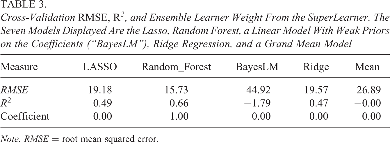
Note. RMSE = root mean squared error.

6.2.2. Proximal validation

To gauge how model trained on the remnant might perform on the matched sample, we conducted proximal validation, described in Section 3.1. First, we constructed a second match, m^big, identical to the first, but allowing each treated subject to match at most 10 control subjects. This resulted in $\sum_{i} 1_{[| {j : m_{j}^{big} = m_{i}^{big}} | = 1]} = 452$ unmatchable distal schools as a training set, and $\sum_{i} (1_{[| {j : m_{j}^{big} = m_{i}^{big}} | = 1]} - 1_{[| {j : m_{j} = m_{i}^{big}} | = 1]}) = 27$ proximal schools as a testing set. We then trained the SuperLearner on the distal schools and computed its prediction accuracy against the proximal schools. The results are displayed in Figure 3. Somewhat surprisingly, the prediction models performed better when trained on the distal schools and tested on the proximal schools than when both the training and testing sets were the entire remnant, as in cross-validation. This may be a result of sampling error or the fact that the distal set contains a number of outlier schools whose AIMS reading scores are particularly hard to predict. These schools will increase the estimated MSE reported by any validation method that includes them in its testing set. If there are no outlier schools in the proximal set, proximal validation will not suffer from this difficulty.

Figure 3.

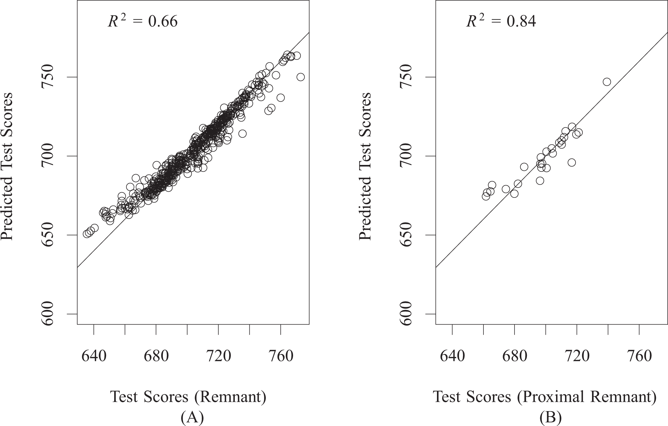
SuperLearner prediction accuracy: predictions ( ${\hat{y}}_{C}$ (X)) as a function of real test scores. (A) The results of the SuperLearner fit to, and tested against, the entire remnant. (B) The proximal validation results: the performance of the SuperLearner fit in the distal portion of the remnant and tested against the proximal portion. The figures also contain the y = x line for comparison.

As an additional check of the identification assumption (Equation 2) for match m, we tested balance on ${\hat{y}}_{C} (X)$ , in the same way as for other covariates: we tested if $E {\hat{y}}_{C}^{T} Z / n_{T} = E {\hat{y}}_{C}^{T} (1 - Z) / n_{C}$ . The resulting p value from the xBalance routine was .46; the balance test on ${\hat{y}}_{C} (X)$ does not falsify Equation 2.

6.2.3. Estimating treatment effects

Finally, we calculated both τ_M, the matching estimator using Y, and ${\hat{τ}}_{rebar}$ , the rebar matching estimator, along with HC3 standard errors, shown in Table 4. To estimate p values, we conducted permutation tests, permuting treatment indicators within matched sets and recomputing the estimates. Ninety-five percent confidence intervals were estimated by inverting the permutation test, as in Rosenbaum (2002a). Neither the conventional method nor rebar detected a statistically significant effect. However, the rebar estimate resulted in a confidence interval with less than half the width of the conventional interval.

Table 4.

The Average Treatment Effect on the Treated τ_ETT, Along With Regression Standard Errors and Permutational p Values and 95% CIs, Estimated With Conventional Propensity-Score Matching, as Described in Section 6.1, and With Rebar

Method	Estimate	SE	p Value	95% CI
PSM	5.91	4.98	0.48	(−10.4, 22.53)
Rebar	1.82	3.65	0.57	(−5.41, 12.17)

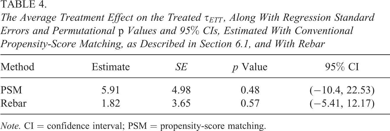
Note. CI = confidence interval; PSM = propensity-score matching.

An anonymous reviewer suggested a post hoc assessment of ${\hat{y}}_{C} (\cdot)$ ’s fit: estimating $R_{M}^{2}$ by comparing y_C from within the match to corresponding predictions ${\hat{y}}_{C}$ . The result was ${\hat{R}}_{M}^{2} =$ .72.

7. Conclusion

In structural engineering, rebar abbreviates “reinforcement bar,” a metal beam that is embedded in concrete. Concrete is resistant to compression, whereas rebar is resistant to tension; the combination of the two materials, rebar and concrete, is robust to a variety of threats. Similarly, the rebar method of this article complements the use of matching for confounder control. Whereas matching typically focuses primarily on possible confounders’ associations with the treatment variable and typically leaves some subjects unmatched, rebar addresses bias by using the the remnant from matching, the unmatched controls, to model possible confounders’ associations with outcomes. The predictions that result, ${\hat{y}}_{C} (x)$ , extract information about subjects’ control potential outcomes from the covariates X . The process of residualizing, that is, subtracting predictions ${\hat{y}}_{C} (x)$ from outcomes Y, can neutralize confounding from variables that the match failed to balance.

Residualizing using the remnant confers these benefits without compromising the statistical rationale for matching. Indeed, matching supplemented with rebar inherits a number of central attractions of the matching estimator. For instance, researchers with any level of statistical training can assess the success of the matching procedure by examining matched units’ comparability on substantively meaningful baseline variables. Although it typically makes use of data from outside the range of common support—the set of subjects i for which 0 < Pr(Z_i = 1|x_i) < 1—its final estimate ${\hat{τ}}_{rebar}$ compares only matched subjects, observing any common support restrictions that the matching procedure observed. The procedure is compatible with postponing analysis involving outcomes until the process of matching is complete, as recommended by Rubin (2008). If matching succeeds in recreating a latent experiment, where subjects matched to each other were assigned to treatment randomly, then ${\hat{τ}}_{rebar}$ , like ${\hat{τ}}_{M}$ , is unbiased.

Generating predictions ${\hat{y}}_{C} (x)$ involves extrapolating from the remnant to the matched sample; in some circumstances, the method could worsen the quality of matched inferences. This risk is mitigated with the use of cross-validation, to limit overfitting of the prediction model, followed by proximate validation, which additionally detects biases specific to extrapolation from lower into higher propensity score regions of x space. Both forms of validation are assisted by the presence of a sizable matching remnant, including at least controls that would have been suitable matches for some treatment group members. While compatible with any method of matching that leaves a positive fraction of the control reservoir unmatched, rebar is particularly attractive in observational studies with many more untreated than treated subjects.

We have focused on the capacity of rebar to reduce bias, but the method may have other benefits as well. For instance, the confidence interval from a rebar analysis of the BES data had less than half the width of the confidence interval from the corresponding matching analysis. Indeed, confidence interval widths and standard errors generally vary inversely with the variance of the outcome. Unless the rebar extrapolation is sufficiently unstable as to worsen MSE—within the matched sample, the mean-square difference between rebar’s out-of-sample prediction and Y exceeds the variance of Y—confidence intervals based on e are bound to be tighter than those based on Y alone. In addition, studies with more stable outcomes tend to have lower design sensitivity (Rosenbaum, 2010; Zubizarreta, Cerdá, & Rosenbaum, 2013). Barring instability, the rebar analysis will be less sensitive to confounding from unmeasured or unmodeled variables. The relative stability of e and Y is reflected in the prediction R² of the rebar ${\hat{y}}_{C} (\cdot)$ when applied to the matched set, for which cross-validation and proximal validation can suggest a plausible range.

Footnotes

8. Appendix Proofs of Propositions 3 and 4

Authors’ Note

The authors gratefully acknowledge support and helpful comments from Brian Junker, Kerby Shedden, Walter Mebane, Sue Dynarski, and three anonymous reviewers.

Declaration of Conflicting Interests

The author(s) declared no potential conflicts of interest with respect to the research, authorship, and/or publication of this article.

Funding

The author(s) disclosed receipt of the following financial support for the research, authorship, and/or publication of this article: Work on this paper was partially supported by a contract with the National Center on Education and the Economy to evaluate the implementation and efficacy of its Excellence for All Initiative and by IES Grant R305B1000012.

Notes

References

Abadie

Imbens

G. W.

(2006). Large sample properties of matching estimators for average treatment effects. Econometrica, 74, 235–267.

Abadie

Imbens

G. W

. (2012). Bias-corrected matching estimators for average treatment effects. Journal of Business & Economic Statistics, 29, 1–11.

Agresti

. (2013). Categorical data analysis. Hoboken, NJ: John Wiley.

Austin

P. C.

(2011). An introduction to propensity score methods for reducing the effects of confounding in observational studies. Multivariate Behavioral Research, 46, 399–424.

Bishop

J. H.

(1997). The effect of national standards and curriculum-based exams on achievement. The American Economic Review, 87, 260–264.

Bishop

J. H.

(2000). Curriculum-based external exit exam systems: Do students learn more? How? Psychology, Public Policy, and Law, 6, 199.

Bowers

Fredrickson

Hansen

(2010). RItools: Randomization inference tools. R package version 0.1-11. Retrieved from http://www.jakebowers.org/RItools.html

Braitman

L. E.

Rosenbaum

P. R.

(2002). Rare outcomes, common treatments: Analytic strategies using propensity scores. Annals of Internal Medicine, 137, 693–695.

Breiman

(2001). Random forests. Machine Learning, 45, 5–32.

10.

Brookhart

M. A.

Schneeweiss

Rothman

K. J.

Glynn

R. J.

Avorn

Stürmer

(2006). Variable selection for propensity score models. American Journal of Epidemiology, 163, 1149–1156.

11.

Cinar

Zubizarreta

J. R

. (2016). Maximizing the information content of a balanced matched sample in a study of the economic performance of green buildings. Annals of Applied Statistics, 10, 1997–2020.

12.

Collier

Millimet

D. L.

(2009). Institutional arrangements in educational systems and student achievement: A cross-national analysis. Empirical Economics, 37, 329–381.

13.

Cox

. (1958). The planning of experiments. New York, NY: John Wiley.

14.

Diamond

Sekhon

J. S.

(2013). Genetic matching for estimating causal effects: A general multivariate matching method for achieving balance in observational studies. Review of Economics and Statistics, 95, 932–945.

15.

Efron

Gong

(1983). A leisurely look at the bootstrap, the jackknife, and cross validation. The American Statistician, 37, 36–48.

16.

Friedman

Hastie

Tibshirani

(2010). Regularization paths for generalized linear models via coordinate descent. Journal of Statistical Software, 33, 1–22.

17.

Gastwirth

Krieger

Rosenbaum

(1998). Dual and simultaneous sensitivity analysis for matched pairs. Biometrika, 85, 907–920.

18.

Gelman

Jakulin

Pittau

M. G.

Y.-S.

(2008). A weakly informative default prior distribution for logistic and other regression models. The Annals of Applied Statistics, 2, 1360–1383.

19.

Gelman

Y.-S.

(2015). Arm: Data analysis using regression and multilevel/hierarchical models. R package version 1.8–5. Retrieved from https://cran.r-project.org/package=arm

20.

Greenland

(2003). Quantifying biases in causal models: Classical confounding vs. collider-stratification bias. Epidemiology, 14, 300–306.

21.

Hansen

B. B.

(2008). The prognostic analogue of the propensity score. Biometrika, 95, 481–488. doi:10.1093/biomet/asn004.

22.

Hansen

B. B.

(2011, 7 15). Propensity score matching to extract latent experiments from nonexperimental data: A case study. In Dorans

Neil J.

Sinharay

Sandip

(Eds.), Looking back: Proceedings of a conference in honor of Paul W. Holland (pp. 149–181). New York, NY: Springer.

23.

Hansen

Ben B.

Klopfer

Stephanie Olsen

. (2006). Optimal full matching and related designs via network flows. Journal of Computational and Graphical Statistics, 15, 609–627.

24.

D. E.

Imai

King

Stuart

E. A.

(2007a). Matching as nonparametric preprocessing for reducing model dependence in parametric causal inference. Political Analysis, 15, 199–236.

25.

D. E.

Imai

King

Stuart

E. A.

(2007b). Matching as nonparametric preprocessing for reducing model dependence in parametric causal inference. Political Analysis, 15, 199–236.

26.

Hoerl

Kennard

(1970). Ridge regression: Biased estimation for nonorthogonal problems. Technometrics, 12, 55–67.

27.

Hosman

C. A.

Hansen

B. B.

Holland

P. W.

(2010). The sensitivity of linear regression coefficients’ confidence limits to the omission of a confounder. Annals of Applied Statistics, 4, 849–870.

28.

Iacus

S. M.

King

Porro

(2011). Causal inference without balance checking: Coarsened exact matching. Political Analysis, 20, 1–24.

29.

Iacus

S. M.

King

Porro

. (2015). Cem: Coarsened exact matching, R package version 1.1.17. Retrieved from https://cran.r-project.org/package=cem

30.

Kang

J. D.

Schafer

J. L.

(2007). Demystifying double robustness: A comparison of alternative strategies for estimating a population mean from incomplete data. Statistical Science, 22, 523–539.

31.

Lee

B. K.

Lessler

Stuart

E. A.

(2010). Improving propensity score weighting using machine learning. Statistics in Medicine, 29, 337–346.

32.

Liaw

Wiener

(2002). Classification and regression by random forest. R News, 2, 18–22.

33.

McCaffrey

D. F.

Griffin

B. A.

Almirall

Slaughter

M. E.

Ramchand

Burgette

L. F.

(2013). A tutorial on propensity score estimation for multiple treatments using generalized boosted models. Statistics in Medicine, 32, 3388–3414.

34.

Middleton

Aronow

(2015). Unbiased estimation of the average treatment effect in cluster-randomized experiments. Statistics, Politics and Policy, 6, 39–75. doi:10.1515/spp-2013-0002

35.

National Center for Education Statistics. (2013). Common core of data (CCD) [electronic resource]. Retrieved October 15, 2013, from https://nces.ed.gov/ccd/

36.

Neyman

(1990). On the application of probability theory to agricultural experiments. Essay on principles. Section 9. Statistical Science, 5, 463–480, transl. by Dabrowska

D. M.

Speed

T. P.

from 1923 Polish original.

37.

Pane

J. F.

Griffin

B. A.

McCaffrey

D. F.

Karam

. (2013). Effectiveness of cognitive tutor algebra I at scale. Educational Evaluation and Policy Analysis. doi:0162373713507480.

38.

Pearl

(2009). Remarks on the method of propensity score. Statistics in Medicine, 28, 1415–1416.

39.

Pimentel

S. D.

Small

D. S.

Rosenbaum

P. R.

(2016). Constructed second control groups and attenuation of unmeasured biases. Journal of the American Statistical Association, 111, 1157–1167.

40.

Polley

van der Laan

. (2014). SuperLearner: Super learner prediction, R package version 2.0–15. https://cran.r-project.org/package=SuperLearner

41.

Rosenbaum

P. R.

(1991). A characterization of optimal designs for observational studies. Journal of the Royal Statistical Society, 53, 597–610.

42.

Rosenbaum

(2002a). Covariance adjustment in randomized experiments and observational studies. Statistical Science, 17, 286–327.

43.

Rosenbaum

P. R

. (2002b). Observational studies (2nd ed.). New York, NY: Springer-Verlag.

44.

Rosenbaum

P. R.

(2010). Design of observational studies. New York, NY: Springer.

45.

Rosenbaum

Rubin

(1983). The central role of the propensity score in observational studies for causal effects. Biometrika, 70, 41–55.

46.

Rubin

D. B.

(1973). The use of matched sampling and regression adjustment to remove bias in observational studies. Biometrics, 29, 185–203.

47.

Rubin

D. B.

(1974). Estimating the causal effects of treatments in randomized and nonrandomized studies. Journal of Educational Psychology, 66, 688–701.

48.

Rubin

D. B.

(1980). Bias reduction using Mahalanobis-metric matching. Biometrics, 36, 293–298.

49.

Rubin

D. B.

(2008). For objective causal inference, design trumps analysis. Annals of Applied Statistics, 2, 808–840.

50.

Rubin

D. B.

Thomas

(1996). Matching using estimated propensity scores: Relating theory to practice. Biometrics, 52, 249–264.

51.

Sekhon

J. S.

(2011). Multivariate and propensity score matching software with automated balance optimization: The matching package for R. Journal of Statistical Software, 42, 1–52.

52.

Sjölander

(2009). Propensity scores and M-structures. Statistics in medicine, 28, 1416–1420.

53.

Steiner

P. M.

Cook

T. D.

Clark

(2015). Bias reduction in quasiexperiments with little selection theory but many covariates. Journal of Research on Educational Effectiveness, 8, 552–576.

54.

Tibshirani

(1996). Regression shrinkage and selection via the lasso. Journal of the Royal Statistical Society. Series B (Methodological), 58, 267–288.

55.

Varadhan

. (2008). [R] How to randomly generate a n by n positive definite matrix in R. Retrieved May 5, 2015, from https://stat.ethz.ch/pipermail/r-help/2008-February/153708.

56.

Venables

W. N.

Ripley

B. D.

(2002) Modern applied statistics with S (4th ed.). New York, NY: Springer.

57.

Wright

M. N.

Ziegler

. (2015). Ranger: A fast implementation of random forests for high dimensional data in C++ and R. arXiv preprint arXiv:1508.044 09

58.

Zorn

(2005). A solution to separation in binary response models. Political Analysis, 13, 157–170.

59.

Zubizarreta

J. R.

Cerdá

Rosenbaum

P. R.

(2013). Effect of the 2010 Chilean earthquake on posttraumatic stress reducing sensitivity to unmeasured bias through study design. Epidemiology (Cambridge, Mass.), 24, 79.

Rebar: Reinforcing a Matching Estimator With Predictions From High-Dimensional Covariates

Abstract

Keywords

1. Introduction: Two Types of Neglected Data

2. Matching in Observational Studies: Review

3. Rebar: Using an Outcome Model to Reduce Bias in a Matching Design

3.1. Cross-Validation and Proximal Validation: Assessing y ^ C ( ⋅ )

4. Rebar’s Effects on Bias

4.1. An Upper Bound on the Bias of the Rebar Estimator

5. A Simulation Study

5.1. Data-Generating Models

5.2. Treatment-Effect Estimators

Optimal pair matching with propensity scores from logistic regression

Nearest-neighbor match with propensity scores from logistic regression

Coarsened exact matching

Optimal pair matching with propensity scores from SuperLearner

5.3. Simulation Results

5.4. Rebar’s Performance Under Nonlinearity

6. Example Data Analysis: Evaluating Board Exam Systems (BES)

6.1. A Propensity Score Match

6.2. Rebar to Adjust the Match

6.2.1. Estimating y ^ C ( ⋅ )

6.2.2. Proximal validation

6.2.3. Estimating treatment effects

7. Conclusion

Footnotes

8. Appendix Proofs of Propositions 3 and 4

Authors’ Note

Declaration of Conflicting Interests

Funding

Notes

References

3.1. Cross-Validation and Proximal Validation: Assessing ${\hat{y}}_{C} (\cdot)$

6.2.1. Estimating ${\hat{y}}_{C} (\cdot)$