Item Response Data Analysis Using Stata Item Response Theory Package

1. Models and Parameterization

First, the irt package takes the raw item responses data organized by individual or the item response pattern data with observed frequency weights. Most of conventional unidimensional parametric IRT models can be estimated for binary (1-, 2-, 3-parameter logistics [PL] models), ordinal (graded response, partial credit, generalized partial credit, and rating scale), and categorical response data (nominal response model) via the package using either the drop-down menu or syntax. However, multidimensional IRT models are currently not supported at least within the package. Other modules such as gllamm (Rabe-Hesketh, Skrondal, & Pickles, 2014) can handle more complex IRT models including multidimensional models, these options are excluded from the current review to focus on the newly developed irt package.

Note that 1-PL model parameterization is essentially the same as a Rasch (1960) model, but the parameterization used in the package is the constrained version of 2-PL model (see Birnbaum, 1968) in which the slopes are constrained to be equal across all items. Therefore, the estimated variance of latent ability in the original Rasch (1960) model should be obtained as the squared estimated slope. For binary response models, discrimination parameters (slopes) and difficulty parameters (thresholds) are printed along with standard errors, observed Z values, p values, and Wald-type 95% confidence intervals (see Figure 1). Intercept parameters and standard errors are not reported; therefore, a separate calculation (e.g., delta method) is needed for users who want to report intercept estimates and corresponding standard errors. In the 3-PL model (Birnbaum, 1968) parameterization, a constant pseudo-guessing parameter is estimated, so item-specific guessing parameters are not obtainable if 3-PL model is checked in the dialogue box. Using a constant guessing parameter, restriction allows more stable and time-efficient estimation of the model without using any prior distribution (see, e.g., Birnbaum, 1968; San Martín, Rolin, & Castro, 2013). It is possible to estimate separate pseudo-guessing parameters with an advance option called hybrid model specification menu or sepguessing in syntax. However, it is expected to yield the less efficient or stable estimation when this feature is used because the package does not allow using prior distribution for guessing parameters unlike other IRT software packages. The manual of Stata irt package also does not encourage of using this feature for 3-PL models either.

OPEN IN VIEWER

Figure 1.

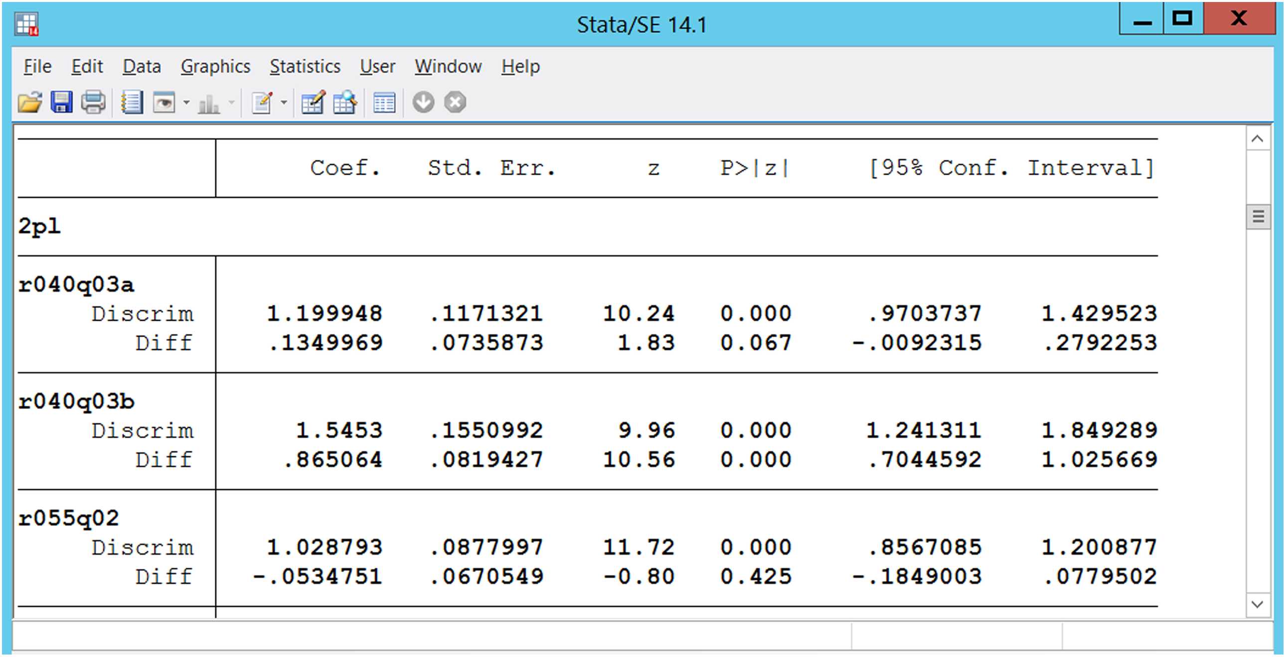
Example of output in the irt package of Stata.

For ordinal response models, the item response data can take the values that start with either 0 or 1 since the software automatically count the number of categories. However, it should be noted that any negative values (e.g., −1, −9, −99) cannot be properly taken as input data, and the program does not run to estimate dichotomous item response models if negative values exist in data sets. For graded response models (GRMs; Samejima, 1969), on the other hand, the program runs with a data set that includes negative values but yields incorrect results. Therefore, users need to pay attention to this coding issue if a GRM is used. It should also be noted that rating scale models (Andrich, 1978a, 1978b) require the same number of categories for all items in the calibration model. The nominal model parameterization in this package follows Bock (1972) and Bakers (1993), and baseline constraints are used for identification of the model taking the lowest category as the reference category. Accordingly, scoring function values are not obtainable directly from the current parameterization. A new parameterization of the nominal model (Thissen, Cai, & Bock, 2010) seems to be useful in further development if the package is planned to be extended toward multidimensional IRT models. Finally, the hybrid model option accommodates mixed-format item response data. To evaluate the performance of hybrid model estimation, we fit the same hybrid model (53 items with 2 PL, 56 items with 3 PL, and 21 items with GRM) for 129 item response data from 3,846 students that are extracted from Programme for International Student Assessment (PISA; Adams & Wu, 2002) 2000 Reading literacy (United States) using the IRT package in Stata and flexMIRT. As shown in Figure 2, the item parameter estimates from both software are almost identical when the guessing parameters are constrained to be the same in flexMIRT. The two sets of standard errors from two software packages are also very close to each other. However, if users would like to estimate different guessing parameters across multiple-choice items, the estimation does not converge within 500 expectation and maximization (EM, Bock & Aitkin, 1981) cycles with flexMIRT because of some of the multiple-choice items that have nearly zero guessing parameters. In this case, priors can be used to stabilize the model estimation, which is not supported in Stata irt package.

OPEN IN VIEWER

Figure 2.

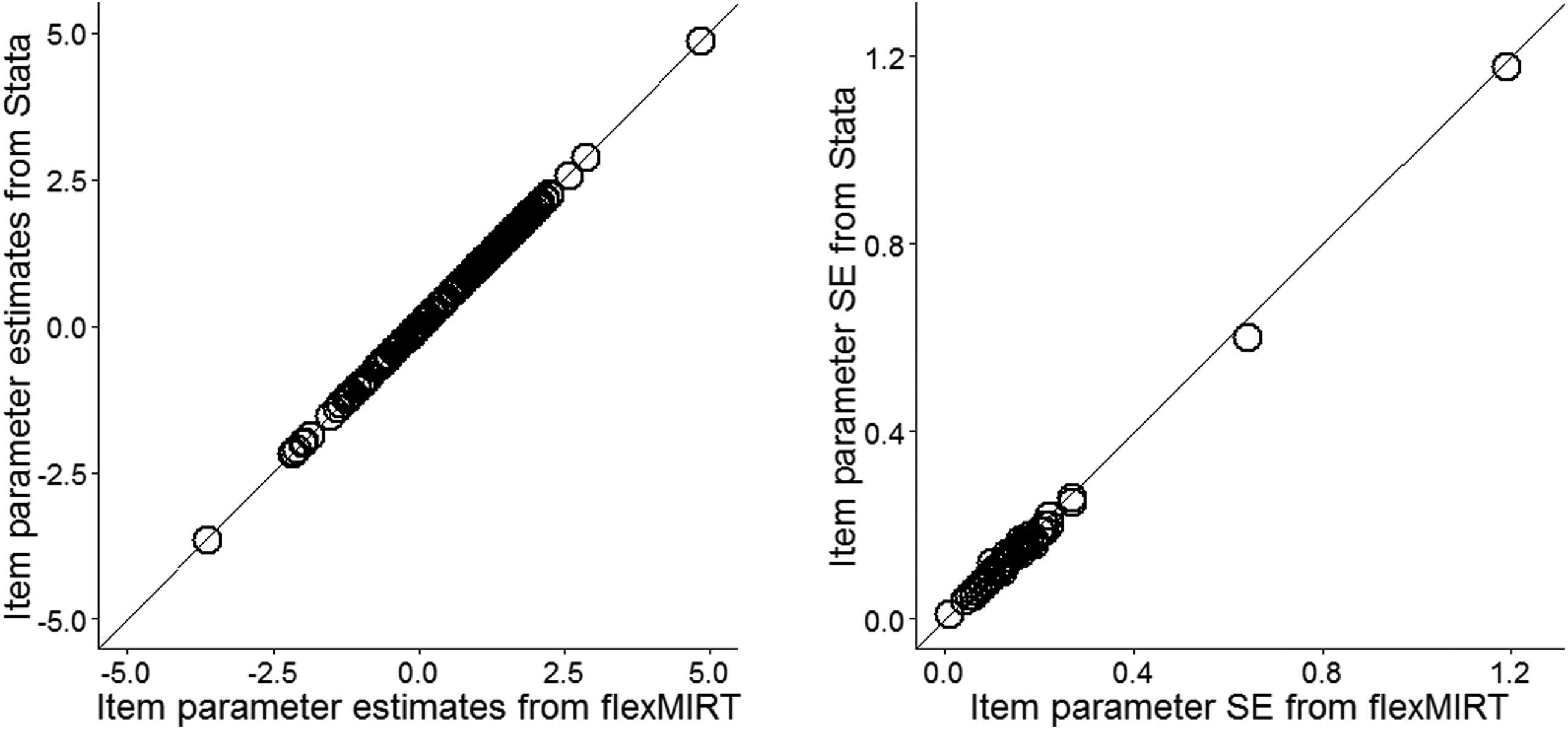
Comparison of item parameter estimates and item parameter estimate standard error from flexMIRT and Stata irt package when the guessing parameters are constrained to be equal using U.S. PISA 2000 Reading literacy data.

With respect to item response data collected from a clustered sample, the model-based approach (e.g., multilevel IRT models) is not supported, but the design-based approach using cluster information can be applied to adjust standard errors. The sample weights can also be incorporated, and standard errors can be calculated using robust cluster option (as known as sandwich estimator, StataCorp LLP, 2015) to address the dependency among individuals within clusters and sample weights properly. We used a simulated item response data from cluster sampling to compare the model estimation results between Stata irt package and Mplus. A total of 20 five-category item responses were simulated with stratified cluster sampling of examinees, where informative sampling weights were generated. As it can be seen in Figure 3, the point estimates are identical up to the second or third decimal point, and standard errors are also very close to each other. Note that the reported standard errors are obtained from using cluster robust standard error option in Stata irt package. More details on standard error options are discussed in Estimation section.

OPEN IN VIEWER

Figure 3.

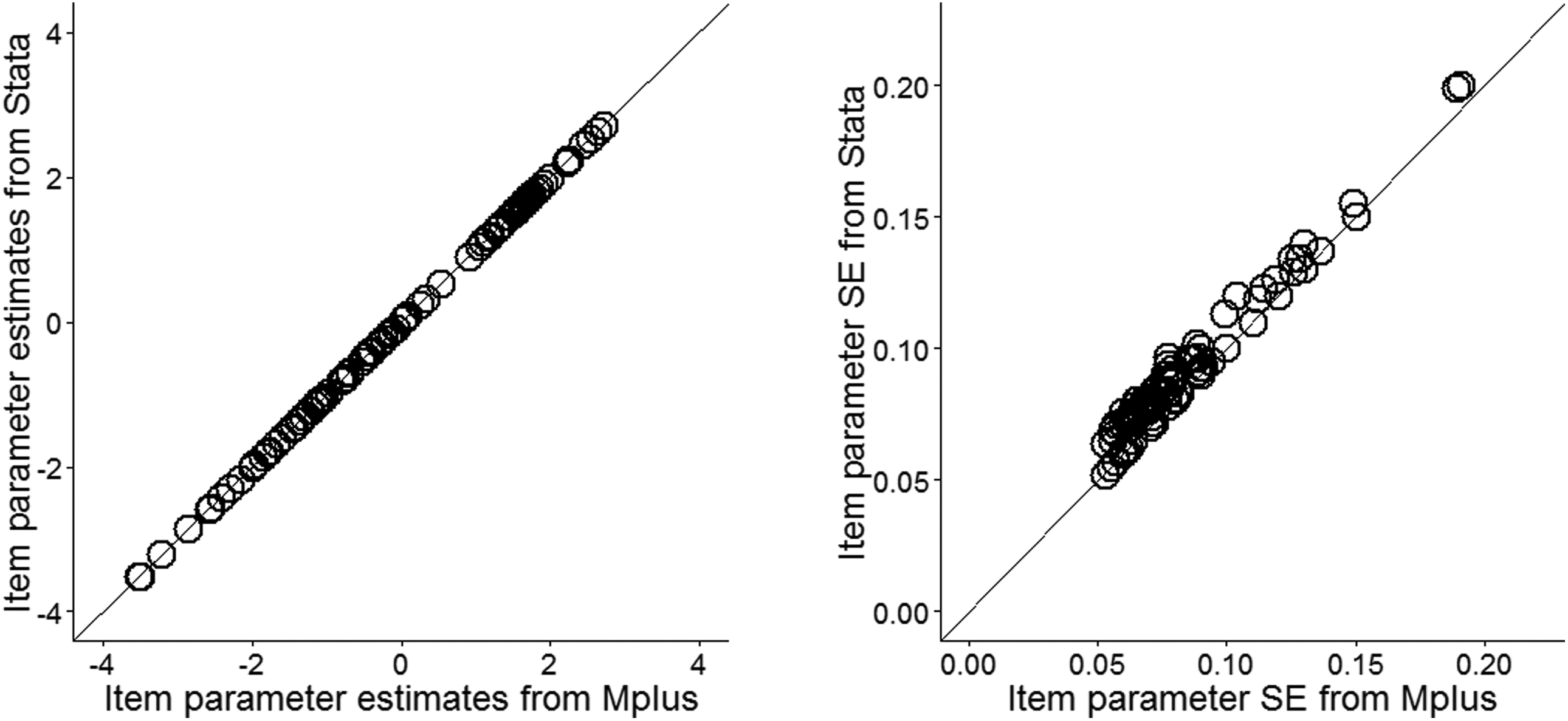
Comparison of item parameter estimates and estimated clustered robust standard errors from Mplus and Stata irt package using simulated data.

2. Estimation

Full information maximum likelihood estimation is the only estimation option for the IRT models supported by the package. Accordingly, missing item responses simply do not contribute to the likelihood, and the estimates are unbiased as long as the missing at random assumption holds. In addition, the listwise deletion is available, though it is not recommended for losing too much information in general. Users need to be mindful that the conventional EM algorithm (Bock & Aitkin, 1981) that is often the default of other IRT software such as mirt R package (Chalmers, 2017), flexMIRT, or Mplus is not available in Stata irt package. Instead, the package supports a couple of Newton-type computation algorithms that users can choose: (modified) Newton–Raphson (default) and other quasi-Newton methods (Berndt–Hall–Hall–Hausman; Broyden–Fletcher–Goldfarb–Shanno algorithm; Davidon–Fletcher–Powell algorithm) in which the Hessian matrix is computed numerically rather than analytically. By default, the package uses analytical formulas for computing the gradient and Hessian for all integration methods.

As for the numerical integration method (intmethod) to calculate the marginal likelihood, two kinds of adaptive Gauss–Hermite (AGH) quadrature methods (mean and variance; mode and curvature) and a nonadaptive (as known as fixed) Gauss–Hermite quadrature method are available. The default setting is the mvagHermitee, mean and variance AGH (Rabe-Hesketh, Skrondal, & Pickles, 2002) with seven quadrature points (QPs). It is unclear why the AGH is chosen as the default over the mode and curvature AGH (Liu & Pierce, 1994). However, we found out that there can be some convergence issues with mode and curvature AGH in our Example 1 (see Figure 4). In general, AGH quadrature can be more time-consuming because the QPs and weights needed to be updated in every iteration and they also depend on the unknown parameters. Therefore, if the parameters are extreme values with large standard errors, the estimation process could take even longer. Given that the models are all unidimensional models, it can be a reasonable idea to use the nonadaptive (as known as fixed) Gauss–Hermite quadrature; however, it should be noted that the users need to increase the number of QPs rather than relying on the default of seven (e.g., larger than 25 which is minimum default for other software packages), when changing the default to the nonadaptive Gauss–Hermite quadrature method. The default convergence criteria are 1e-4 for maximum likelihood estimators and 1e-5 for scaled gradient.

OPEN IN VIEWER

Figure 4.

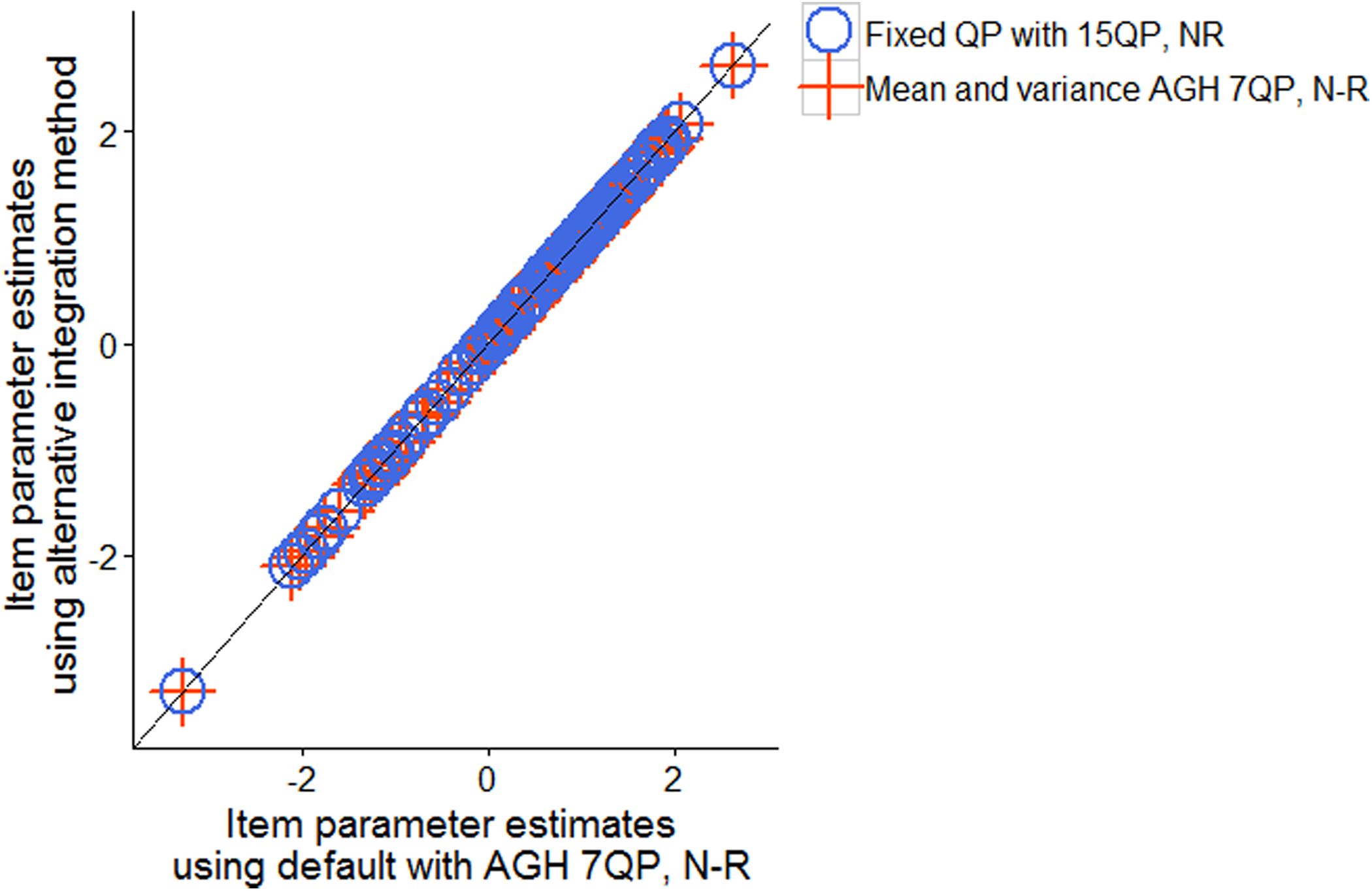
Comparison of item parameter estimates from different computation algorithms available in Stata irt package.

The iteration process prints out fixed-effect estimation stage history and full model estimation stage history. The fixed-effect estimation stage is to calculate starting values for item parameter estimates. Using startvalues() options, users can specify how starting values are calculated and the syntax might be useful if starting values need to be changed. In addition, the number of iterations for the fixed-effect estimation can be manipulated by users. If users are interested in what the starting values are, noestimate can be used to print out starting values before full estimation begins. Given that starting values are crucial when the Newton–Raphson family algorithms are used, this feature could be useful for further complex modes or data.

To demonstrate model estimation, we compared the performance of estimation of unidimensional 2 PL with an empirical data set extracted from PISA. We estimated the model with modified Newton–Raphson algorithm with three different integration methods, namely, default AGH 7QP, mode and variance AGH 7QP, and fixed QP with 15QP. The mode and variance AGH failed in convergence, so the estimation results from three methods are reported in Figure 4. In terms of time efficiency, it took about 27 s with the AGH and 43 s with fixed QP. The difference is not substantial since the fitted model was unidimensional. On the other hand, other quasi-Newton methods either took a long time or failed in estimating the model for this large data.

Standard error options include observed information matrix (default), robust, clustered robust, bootstrap, and jackknife. Among the approximation of the observed information matrix, analytically obtained Hessian is used as the default. The sandwich estimator can be obtained when robust is chosen. Clustered robust can be also used along with a cluster variable when the respondents are nested within clusters. Bootstrap and jackknife methods are also available.

We analyzed the same data set assuming either simple random sampling or clustered sampling. The left graph in Figure 5 summarizes the standard errors from default, robust, and bootstrap method with 50 replications. The jackknife option could not produce standard errors within 24 hrs with over 3,000 examinees, so the results from this option are not reported here. On the other hand, the standard errors that take clustered sampling into account are reported in the right panel of Figure 5. In applications for nested data like PISA, literature (e.g., Rust, 1985) recommend to consider the violation of independency and adjust the standard errors using clustered robust, jackknife, and bootstrap. The clustered robust option is recommended for time efficiency.

OPEN IN VIEWER

Figure 5.

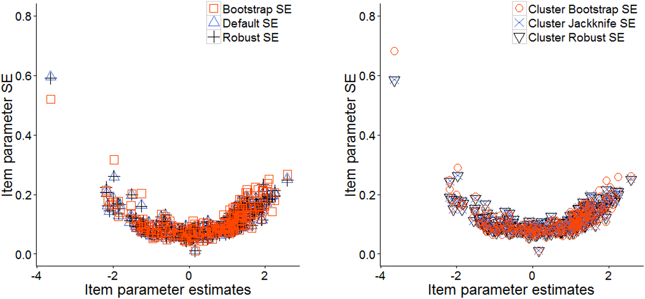
Comparison of standard errors available in Stata irt package.

3. Model Fit Assessment

In IRT applications such as scoring or testing differential item functioning (DIF), model-data fit assessment is crucial because those applications heavily rely on the parametric IRT models. Therefore, we also review what kind of model fit indices are available in the package. While the dialogue box allows users to estimate models without using command lines, all of the information related to model fit assessment should be obtained by using either a predefined postestimation command (e.g., estat ic) or multiple lines of commands to calculate or to visualize the fit. The standard command estat ic and a likelihood ratio test for nested models are also possible using command lrtest. In addition, estat ic prints out likelihood-based Akaike’s and Schwarz’s Bayesian information criteria. However, absolute model fit indices for IRT models such as Pearson’s χ² and likelihood ratio (G ²) or the root mean square error of approximation are not immediately available but need to be calculated using the saved information such as expected proportion of the responses. The package manual suggests to plot the item characteristic curve and observed proportion of the responses on the sample plot and examine the fit visually. As the manual provides sample commands to draw item characteristic curve (irtgraph icc) and observed proportion of responses, researchers can easily implement and produce the necessary plots. However, it would be much more useful for users if they could obtain at least conventional full information fit indices like χ² and G ². In addition, since the full information fit indices are not obtainable or perform very poorly when the number of items and the number of categories are large due to sparse contingency tables, further consideration of limited information fit indices (e.g., Cai & Hansen, 2013; Maydeu-Olivares & Joe, 2005) will be very helpful for users. Given that further analysis like measurement invariance or DIF analysis is valid only when the models are reasonably correct, providing enough information on model fit assessment is an important capacity of the software. In addition, conventional unidimensional IRT model assumptions (e.g., local dependence or latent distribution) can be tested. For example, item-level fit assessment (Orlando & Thissen, 2000) or pairwise fit assessment can be further useful. These can be written as a command attached to irt package or provided as macros for users. It seems that the package deserves further development with respect to providing more useful information to assess the models.

4. Differential Item Functioning

Two different approaches to test differential item functioning (DIF) are supported; however, it should be noted that none of these are within the IRT framework. The first implemented method is called logistic regression procedure that can be executed using either dialogue box or command diflogistic (see Swaminathan & Rogers, 1990, for more details). This method does not directly compare the item characteristic curves (item parameter estimates) but compares nested logistic regression models in that the probability of the item correct is regressed on observed group variable and estimated latent trait. Using the interaction term between the two predictors, nonuniform DIF can be also detected. Both uniform and nonuniform DIF are tested and reported along with χ² values and p values. The second available method is Mantel–Haenszel (M-H) using difmh that produces χ² values and odds ratio for only dichotomously scored items. This test only applies to detect uniform DIF, however. The M-H test is to examine the independency between two dichotomous variables conditioned on a third variable (often summed scores; see Mantel & Haenszel, 1959; Holland & Thayer, 1988, for details). Given that the multiple-group IRT analysis is a very common application of IRT for either concurrent calibration or DIF testing, the most urgent aspect that requires development seems to be the multiple-group analysis feature that accommodates IRT DIF analysis.

5. IRT Scoring

Scoring is another important purpose of IRT applications. For latent trait estimators, empirical Bayes means (default) and modes are available. Those correspond to expected a posteriori and maximum a posteriori, respectively. Maximum likelihood scores are not supported. To obtain the latent scores and standard errors, one should look for predict-prediction after estimation menu, which is shown in Figure 6. To obtain standard error of the latent scores, empirical Bayes estimator, the check box to generate a new variable for standard errors needs to be checked. The feature of predicted probabilities is helpful to compare these against observed probabilities and evaluate the item- and model-level fit assessment.

OPEN IN VIEWER

Figure 6.

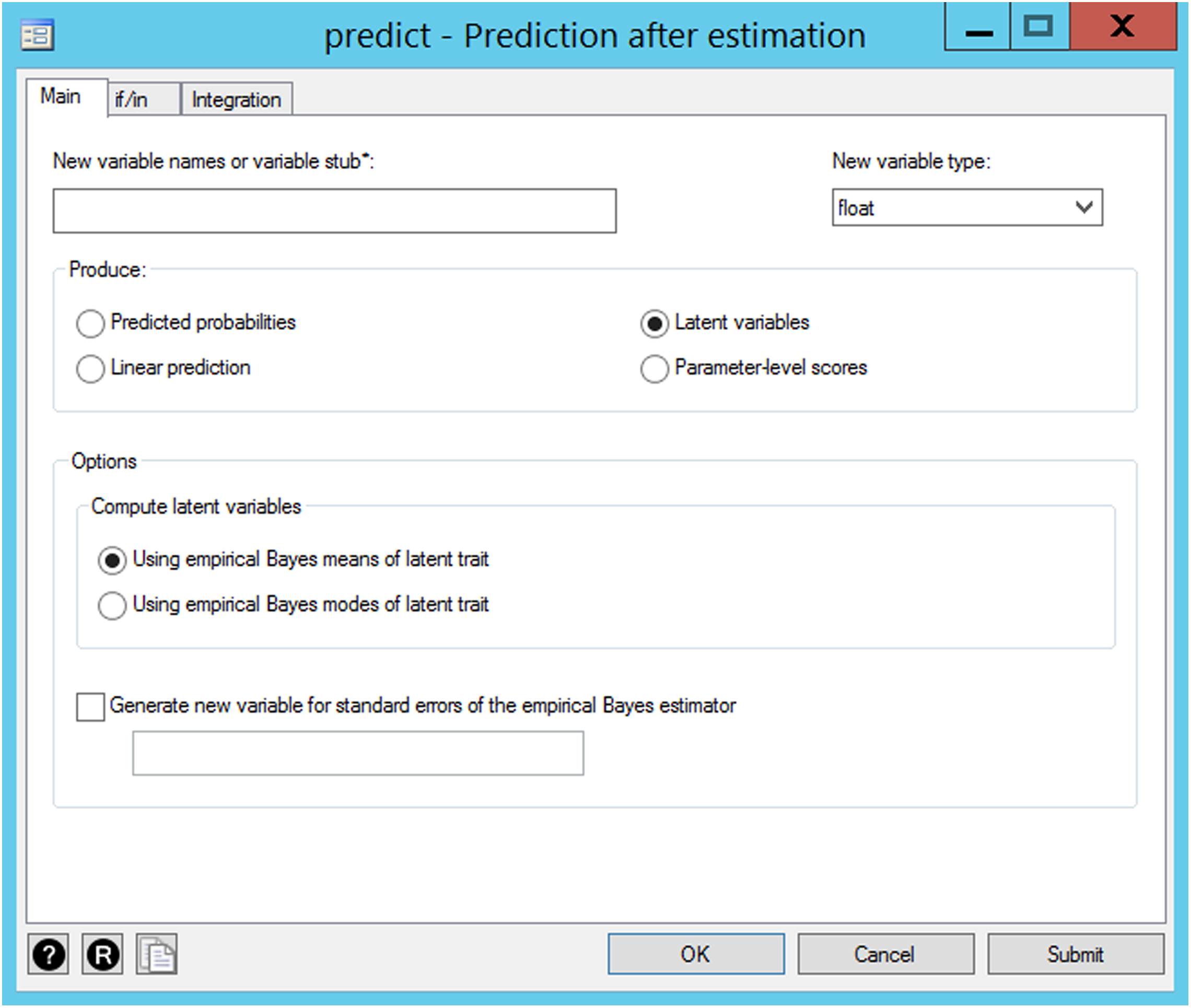
Item response theory (IRT) scoring drop-down menu available in irt package.

6. Report and Graphic Features

The features of report and graphic of the package are convenient because additional formatting processes of the results can be minimized. For example, sorting and grouping of the results by item or specific parameter magnitude are possible in report. Graphic menu as well as postestimation commands provides item characteristic curves, category characteristic curves (irtgraph icc), test characteristic curves (irtgraph tcc), item information curves (irtgraph ifc), and test information curves (irtgraph tfc). Customization options are also useful to add additional lines (e.g., vertical lines for difficulty parameters) or standard errors (use se in command). The color or thickness of lines and labels for the axes can be easily changed by the users. The figures can be saved as portable network graphics, portable document format, Stata’s graph files, or meta files and used for documents generated by either Microsoft word or LaTeX.

7. Other Features

For advanced users, user-defined estimation environment or constraints are often needed. Some limited user-defined environment or constraints are available through commands. The estimation conditions such as convergence criterion, number of QPs, and the maximum number of iterations can be all controlled by the user. However, it is not possible for users to impose some user-defined constraints such as linear constraints or equality constraints on item parameter estimates. It is possible to obtain constraints matrix, but it is unclear if we users can change the constraints matrix called by e(Cns). While fitting a model with constrained parameters might not be flexible, testing the linear and nonlinear combination of coefficients is still well facilitated by nlcom and lincom. In addition, variance–covariance matrix of estimators can be obtained using estat vce; therefore, further application such as characterizing uncertainty in IRT scores using multiple imputation-based approach (Yang, Hansen, & Cai, 2012) or adjusting standard errors via analytical approach (e.g., Cheng & Yuan, 2010). Finally, we were interested in how the package can be used for simulation studies. While the package itself does not facilitate simulating data directly, the combination of R packages, Rstata and foreign, can support Monte Carlo simulation studies efficiently as long as the IRT models are available in the irt package. An example code is provided in Appendix.

8. Conclusions

It seems that the irt package in Stata is convenient for the applied researchers who have used Stata for their routinely conducted data analyses. Although it is limited to unidimensional IRT models, the package functions as a good platform where users can calibrate and score item response data. In addition, the graphical features will be well appreciated by the users. For applied researchers, making more information on model assessment available and adding a multiple-group analysis module are very useful. From a methodological researcher’s perspective, the package needs to consider multidimensional models and different parameterization with respect to the nominal response models. Most of all, allowing more user-defined environment and constraints would be appreciated by more advanced IRT users.