Detecting Aberrant Behavior and Item Preknowledge: A Comparison of Mixture Modeling Method and Residual Method

Abstract

The modern web-based technology greatly popularizes computer-administered testing, also known as online testing. When these online tests are administered continuously within a certain “testing window,” many items are likely to be exposed and compromised, posing a type of test security concern. In addition, if the testing time is limited, another recognized aberrant behavior is rapid guessing, which refers to quickly answering an item without processing its meaning. Both cheating behavior and rapid guessing result in extremely short response times. This article introduces a mixture hierarchical item response theory model, using both response accuracy and response time information, to help differentiate aberrant behavior from normal behavior. The model-based approach is compared to the Bayesian residual-based fit statistic in both simulation study and two real data examples. Results show that the mixture model approach consistently outperforms the residual method in terms of correct detection rate and false positive error rate, in particular when the proportion of aberrance is high. Moreover, the model-based approach is also able to correctly identify compromised items better than residual method.

Keywords

response time aberrant behavior item preknowledge person-fit mixture model item response theory

1. Introduction

Modern web-based technology has greatly popularized computer-administered testing, which is also known as online testing. For instance, in educational assessment, 44 states currently have operational or pilot versions of online tests for their statewide or end-of-course assessment (Dean & Martineau, 2012). In employment settings, many organizations have provided Internet-based assessment for job applicants in personnel selection and recruitment (Lievens & Chapman, 2009; Sackett & Lievens, 2008). To ensure test scores are reliable and valid, statistical procedures for detecting aberrances are essential to identify flaws in the design of a test or irregular behavior of the test takers. Aberrances usually come in different forms such as bad test items, ambiguous instructions, special accommodated examinees, speededness of the test, answer coping, and test cheating. The focus of this article is particularly on the identification of aberrances in online testing that exemplifies as extremely short response times, which usually imply cheating or rapid guessing behaviors.

Taking cheating as a form of aberrant behavior, it is defined as any activity that violates the established rules governing the administration of a test (Cizek, 1999). Different from the answer-copying or answer-changing behavior that is normally seen with paper-and-pencil test, the security breach of online and/or adaptive testing is often due to the item overexposure. This is because online testing is usually administered to small groups of examinees at frequent adjacent time intervals within a certain “testing window,” known as “continuous administration.” As a result, examinees who take the test earlier may share information with those who take it later, imposing the risk that items may become known to many examinees before they take the test (Wang, Zheng, & Chang, 2014). When some items become less difficult over a defined life span, it is reasonable to believe that the performance changes are because of its content having been distributed outside valid usage boundaries (such as published in unauthorized testing review guides), and these items are usually called compromised items. Compromised items should be duly detected, removed, and replenished by new items to ensure test security and validity.

Another commonly observed type of aberrant behavior is rapid guessing (Wang & Xu, 2015; Wise, 2017; Yang, 2007), which is defined as quickly obtaining an answer without carefully processing the meaning of the item (Wise & Kong, 2005). It occurs either due to test speededness or lack of motivation. In the former situation, rapid guessing often happens toward the end of the tests, whereas in the latter situation, rapid guessing can happen on any item. Compared to cheating behavior, rapid guessing also results in extremely short response times, but with a much lower correct response probability. The main objective of this article is not to differentiate cheating behavior from rapid guessing but rather to differentiate aberrant behavior from normal solution behavior. As the article unfolds below, two methods will be compared in terms of their power of detecting aberrant behavior, namely, the mixture hierarchical modeling approach and the Bayesian residual method. The two methods will also be evaluated with respect to their power of detecting item compromise when cheating is a concern.

In what follows, we will briefly review the existing methods for aberrance detection within the framework of residual analysis. We will then review the mixture modeling approach relevant for detection of aberrant behavior and introduce van der Linden’s (2007) hierarchal model that forms the basis of the mixture model.

1.1. Residual Analysis

Detecting test takers’ aberrant behavior and item compromise (we also use item preknowledge exchangeably hereafter) are pivotal to correctly interpret test scores. The traditional approach of detecting aberrant behavior at the person level is to analyze the response vectors for patterns of unexpected responses. This type of analysis is known as person-misfit analysis (McLeod & Lewis, 1999; Meijer & Sijtsma, 1995; van Krimpen-Stoop & Meijer, 2000) and belongs to the broader class of problems of outlier detection (or residual analysis) in statistics. In a review paper by Meijer and Sijtsma (2001), they showed that there are over 40 available statistics to evaluate person-fit. Key to this approach is the availability of a psychometric model that adequately represents regular behavior. Karabatsos (2003) evaluated the performance of 36 person-fit indices side by side, and one main finding in Karabatsos (2003) is that when the proportion of aberrant behavior increases, the power of correct detection drops. This is unsurprising because the reference formed by the “remaining examinees” is contaminated. This is in fact the limitation shared by almost all person-fit indices because when the proportion of aberrancy increases, the separation between normal and aberrant observations is blurred, making the outlier detection harder.

While all person-fit indices reviewed in Meijer and Sijtsma (2001) and Karabatsos (2003) are constructed from response patterns, it was soon realized by researchers that response time (RT) provides additional information to help detect aberrant behavior (e.g., Marianti, Fox, Avetisyan, & Veldkamp, 2014; van der Linden & Guo, 2008; van der Linden & van Krimpen-Stoop, 2003). When assessments are delivered via computer-based devices, collecting response times for each item and person combination becomes straightforward. The benefit of RT usually comes in two different forms including (1) improving the precision of both item (van der Linden, Klein Entink, & Fox, 2010) and person parameter estimation (e.g., Wang, Fan, Chang, & Douglas, 2013b), such that the discrepancy between observation and model prediction from aberrant responses becomes more prominent due to more precise “model prediction” and (2) constructing residuals based on RT (van der Linden & van Krimpen-Stoop, 2003) because aberrant behavior usually manifests itself by irrationally shorter RT.

Several person-misfit indices using RTs were proposed. For example, Marianti, Fox, Avetisyan, and Veldkamp (2014) proposed a Bayesian standardized person-fit index based solely on RT and it worked well in both simulation and real data analysis. On the other hand, van der Linden and van Krimpen-Stoop (2003) proposed to construct residuals based on both responses and RTs and seek for a combination of undesirably negative residual for RTs and positive residual for responses as indicators of item preknowledge. They considered both classical and Bayesian checks when constructing the residuals. For classical checks, the detection rate is .30 and the false-alarm rate is .05. For Bayesian checks, the detection rate doubled relative to the classical checks, but at the cost of a considerable increase in the false-alarm rate. Later, van der Linden and Guo (2008) proposed a fully Bayesian procedure based on the hierarchical model of van der Linden (2007). The primary idea is to form a posterior predictive distribution of RTs as a reference distribution to which the actual RT is compared. This distribution of RTs is constructed based on information accrued through RTs and responses on all other administered items. If the actual RT is too small relative to the posterior predictive distribution, this implies the potential aberrant behavior. Note that because this index is computed for each person-by-item encounter, it can be aggregated at either person level or item level to flag aberrant examinees or to detect item compromise (Qian, Staniewska, Reckase, & Woo, 2016). In this regard, no separate item-misfit index is needed. Their index will be used as a reference to which the mixture modeling approach is compared.

1.2. Mixture Modeling Approach

Different from detecting aberrance via residuals, another commonly seen approach is to directly model the aberrant behavior (rapid guessing behavior mostly) using mixture models. Earlier, only response information enters into the mixture model (e.g., Bolt, Cohen, & Wollack, 2002; Boughton & Yamamoto, 2007; Chang, Tsai, & Hsu, 2014; Goegebeur, De Boeck, Wollack, & Cohen, 2008). For instance, Bolt, Cohen, and Wollack (2002) classify examinees into one of the two classes: speeded or nonspeeded, and all examinees who belong to the speeded class tend to engage in solution behavior at first but switch to rapid guessing behavior at the same fixed switching point. Boughton and Yamamoto’s (2007) HYBRID model allows individual change-point locations for different examinees, and thus, it is more flexible. Goegebeur, De Boeck, Wollack, and Cohen (2008) further propose a speeded item response theory (IRT) model, and their model includes an examinee-specific change-rate parameter, such that it models a smooth, gradual switch from solution behavior to rapid guessing. Of note, a common assumption shared among all these models is that just one change point appears in the entire test-taking process.

In parallel, various mixture models have been proposed to represent divergent RT distributions from solution behavior and rapid guessing such as the two-state model by Schnipke and Scrams (1997) and the effort-moderated IRT model by Wise and DeMars (2006). In particular, when the two types of behaviors coexist, the resulting RT distribution is likely bimodal, and the two-state model intends to curve fit the bimodal shape of RT distribution (Schnipke & Scrams, 1997). Each item therefore has two sets of parameters quantifying the lognormal RT distributions from the two behaviors. However, person parameters are not included in the model, and hence, the model is suitable for evaluating speededness of a test but not suitable for detecting rapid guessing behavior at person level.

Very recently, a few mixture models have been proposed that take into account both RT and response information. For instance, Meyer’s (2010) model assigns examinees to either a speeded or a nonspeeded latent class with each latent class having separate item and population mean/variance parameters. However, the classification is at person level that provides no clue on which item rapid guessing actually happens. Wang and Xu (2015) propose a mixture hierarchical model that can differentiate rapid guessing from solution behavior for each item by person encounter. Their model includes a latent indicator variable that implies the underlying behavior of the test taker on a specific item, whether it be normal (solution based) behavior or rapid guessing behavior. Our model bears close resemblance to Wang and Xu’s model, but the main difference is we replace their person-level guessing propensity parameter (π_i ) by an item-level parameter π_j . The justification is, in case of cheating, items that are overexposed are more likely to be compromised, yielding higher π_j . In case of rapid guessing, items that are placed toward the end of the tests are more likely to be rapidly guessed on, also leading to higher π_j . In addition, different from Wang and Xu (2015), another main objective of this article is to compare the performance of mixture modeling approach versus the Bayesian residual method side by side.

As emphasized earlier, residual analysis is theoretically underpowered if a certain, nonignorable proportion of examinees exhibit aberrant behavior. Therefore, it will be important to check the conditions under which the Bayesian residual method will perform equally, better, or worse than the mixture modeling approach in terms of detecting aberrant behavior at person level, as well as identifying item preknowledge at item level.

2. Method

2.1. A Mixture Hierarchical Model

When modeling responses and RTs jointly (e.g., van der Linden, 2007; Wang, Chang, & Douglas, 2013a; Wang et al., 2013b), the hierarchical model of van der Linden (2007) is by far one of the most popular models for responses and RTs, and this model has become the standard approach to model responses and RTs in standardized testing (Ranger, 2013).

As the name entails, the core of van der Linden’s (2007) model is a hierarchical structure that integrates the responses and RTs through a second-level covariance structure. In particular, the two levels are (1) a measurement model level, wherein RT follows a lognormal model and response accuracy comes from a three-parameter logistic (3PL) model and (2) a subject model that specifies correlation between speed and ability at a population level.

In adhering to the conventional notation, let a_j , b_j , and c_j denote the item discrimination, difficulty, and pseudoguessing¹ parameters for item j, and let θ_i denote the ability for person i, then the probability that person i answers item j correctly using “solution-based” behavior is summarized by the 3PL model as follows:

P (Y_{i j} = 1 | θ_{i}) \equiv P_{j} (θ_{i}) = c_{j} + \frac{1 - c_{j}}{1 + exp [- a_{j} (θ_{i} - b_{j})]} .

Other IRT models, such as the 2PL model, 1PL model, partial credit model, or graded response model, can be supplied in this framework depending upon the nature of the assessment and the type of responses collected (i.e., either dichotomous or polytomous responses).

In parallel with the parameterization in Equation 1, let α_j and $β_{j}$ denote the discrimination power and time intensity of item j with respect to RTs, and let τ_i denote the latent speed parameter of person i. The RT person i spends on item j, t_ij , follows a lognormal distribution. That is, the log-transformed RT follows a normal distribution as

log (t_{i j}) | τ_{i} \sim N (β_{j} - τ_{i}, α_{j}^{- 2}) .

As seen from Equation 2, items with higher time intensity (i.e., larger $β_{j}$ ) require longer time to finish, items with higher discrimination power (i.e., larger α_j ) better distinguish fast and slow responders, and persons with faster speed (i.e., larger τ_i ) spend shorter time on items. When test takers engage in solution behavior, the resulting item RT distribution is usually positively skewed, making lognormal model an ideal choice. However, other parametric models (Rouder, Sun, Speckman, Lu, & Zhou, 2003) and semiparametric models (Wang et al., 2013a, 2013b) are also available whenever the lognormal model shows poor fit.

At the second level, it is assumed that the latent ability and speed parameters, $ξ_{i} = {(θ_{i}, τ_{i})}^{T}$ , follow a bivariate normal distribution with a mean vector of $μ_{p} = (μ_{θ}, μ_{τ})$ , and a covariance matrix of $\sum_{p} = [\begin{matrix} σ_{θ}^{2} & σ_{θτ} \\ σ_{θτ} & σ_{τ}^{2} \end{matrix}]$ . The covariance parameter $σ_{θτ}$ can be either positive or negative, and positive covariance means more able test takers tend to work faster. Throughout this article, the boldface notation denotes both vectors and matrices.

The mixture model is a natural extension of van der Linden’s (2007) hierarchical model. Let $Δ_{i j}$ denote whether person i has aberrant behavior on item j, $Δ_{i j} = 1$ indicates aberrant behavior and $Δ_{i j} = 0$ otherwise. The observed RT, $T_{i j}^{obs}$ , is assumed to have a decomposition as

T_{i j}^{obs} = (1 - Δ_{i j}) T_{i j} + Δ_{i j} C_{i j} .

$T_{i j}$ is the RT for person i on item j from a solution-based behavior, and it follows a lognormal distribution specified in Equation 2; $C_{i j}$ denotes the time person i spends on item j using aberrant behavior. $C_{i j}$ is also assumed to follow a lognormal distribution, but with a common mean parameter of µ_c and a variance of $σ_{c}^{2}$ . This treatment implies that the time spent on an item via cheating or rapid guessing behavior does not depend on either person’s speed or item’s time intensity.² Similarly, the correct response probability of person i on item j can be written as

P (Y_{i j} = 1 | Δ_{i j}, θ_{i}) = P (Y_{i j} = 1 | θ_{i}, a_{j}, b_{j}, c_{j}, Δ_{i j} = 0) (1 - Δ_{i j}) + d_{j} Δ_{i j} .

In Equation 4, when the person engages in solution behavior, the correct response probability follows the typical 3PL model in Equation 1; otherwise, the correct response probability is quantified by d_j . For compromised items, d_j might be close to 1 because the chance of answering a compromised item correctly should be high, regardless of the item difficulty or person’s ability level. If a person engages in rapid guessing, d_j will be close to the chance level of one over the number of options for a multiple-choice item.

Imitating van der Linden’s (2007) hierarchical structure, the latent ability and speed parameters, $ξ_{i} = {(θ_{i}, τ_{i})}^{T}$ , in this mixture model also follow a bivariate normal distribution. The aberrance indicator, $Δ_{i j}$ , is assumed to be dependent on an item-level parameter via $π_{j} = P (Δ_{i j} = 1)$ , in which $π_{j}$ is defined as the propensity of item j being compromised or rapidly guessed on. When cheating is of concern for high-stakes tests, then items that have longer time in use will have higher chance of being compromised, hence higher π_j , than newer items. When rapid guessing happens due to lack of motivation, then π_j is likely just be a random value bounded between 0 and 1.

Please note that in our mixture model, we used item level parameter, π_j , to indicate the propensity of item being problematic, whereas Wang and Xu (2015) used a person-level parameter, π_i . The decision between two model parameterizations should be made with caution. If a test contains items with different features, such as old and new items, then a model with π_j makes more sense. On the other hand, if the test is given to a heterogeneous sample in which the examinees’ test-taking behaviors may differ dramatically (i.e., students with different backgrounds or motivations), then a model with π_i is more appropriate. Depending upon the type of mixing proportion parameter included in the model, item-level or person-level covariates can be included in the future to predict the severity of aberrance. With our model set up, the estimated ${\hat{π}}_{j}$ can be used to indicate item compromise.

In sum, the parameters that need to be estimated in model calibration include item parameters, $a_{j}, b_{j}, c_{j}, d_{j}, α_{j}, β_{j}$ , $π_{j} (j = 1, \dots, j)$ , µ_c , and $σ_{c}^{2}$ ; person parameters, θ_i , and τ_i (i = 1,…, N); the latent indicator, $Δ_{i j}$ ; and the population parameters $σ_{τ}^{2}$ and $σ_{θτ}$ . The constraints $μ_{θ} = 0, μ_{τ} = 0, σ_{θ}^{2} = 1$ are imposed to ensure model identifiability (Wang & Xu, 2015). The typical local independence assumptions in IRT still hold here. That is, the responses and response times on all items for a person are locally independent conditioning on θ_i , τ_i , and $Δ_{i j}$ . In addition, for item j with π_j , $Δ_{i j}$ are identically and independently distributed (i.i.d.) Bernoulli trials. A fully Bayesian Markov chain Monte Carlo (MCMC) algorithm is developed for model calibration. In the rth iteration of MCMC, the aberrance indicator, $Δ_{i j}$ , is updated for each i and j based on its posterior distribution, which is a Bernoulli distribution with parameter $p_{i j}^{r} = P (Δ_{i j}^{r} = 1 | all other model parameters)$ . This parameter is a function of all model parameters from the (r − 1)th iteration; for details, please refer to the Online Appendix (e.g., Equation S1–S6 in the Online Appendix). Within each iteration of the Markov chain, if $p_{i j}^{r} \geq p_{Δ}$ , then ${\hat{Δ}}_{i j} = 1$ , and 0 otherwise. Then, average over the post burn-in iterations of the ${\hat{Δ}}_{i j}$ chain to obtain $\hat{P} ({\hat{Δ}}_{i j} = 1)$ . Here, $\hat{P} ({\hat{Δ}}_{i j} = 1)$ is considered the average posterior probability of ${\hat{Δ}}_{i j} = 1$ , after taking into account the uncertainty of passing the cutoff of $p_{Δ}$ in each iteration of the Markov chain. Then, compare $\hat{P} ({\hat{Δ}}_{i j} = 1)$ to another cutoff $π_{Δ}$ . If $\hat{P} ({\hat{Δ}}_{i j} = 1) \geq π_{Δ}$ , then the (i, j) pair is flagged as aberrant. Usually, both $p_{Δ}$ and $π_{Δ}$ can be fixed at 0.5. The detailed algorithm is provided in the Online Appendix. The full code is written in R (R core team), and it is available from the authors upon request.

2.2. Bayesian Residual Analysis

As a comparison to the mixture modeling approach, the Bayesian residual method (van der Linden & Guo, 2008) is introduced in this subsection. To be specific, let $t_{i j}^{*}$ denote the log-transformed observed RT for person i and item j, the “asterisk” denotes log-transformed RT. Let $t_{(i / j)}^{*}$ and $y_{i / j}$ , respectively, denote the vector of log-time and the vector of responses for person i on all items except item j. After fitting the data with the nonmixture hierarchical model, we compute the posterior predictive density of ${\tilde{t}}_{i j}^{*}$ (denote the model predicted log-time) as

f ({\tilde{t}}_{i j}^{*} | t_{i / j}^{*}, y_{i / j}) = \int f ({\tilde{t}}_{i j}^{*} | τ_{i}) f (τ_{i} | t_{i / j}^{*}, y_{i / j}) d τ_{i} .

In Equation 5, $f ({\tilde{t}}_{i j}^{*} | τ_{i})$ is the lognormal density of ${\tilde{t}}_{i j}^{*}$ , given τ_i that can be obtained from Equation 2. The term $f (τ_{i} | t_{i / j}^{*}, y_{i / j})$ is the posterior density of τ_i given responses and RTs, and it is computed as:

\begin{array}{l} f (τ_{i} | t_{i / j}^{*}, y_{i / j}) \propto f (t_{i / j}^{*} | τ_{i}) f (τ_{i} | y_{i / j}) = [\prod f (t_{i / j}^{*} | τ_{i})] f (τ_{i} | y_{i / j}), \end{array}

where $f (τ_{i} | y_{i / j}) = \int f (τ_{i} | θ_{i}) f (θ_{i} | y_{i / j}) d θ_{i}$ . Assuming ${\hat{θ}}_{i}$ from the IRT model follows a normal distribution, which is often the case when test length is long, the posterior predictive distribution in Equation 5 is normal with a mean of

β_{j} - \frac{\frac{σ_{θτ}}{σ_{τ}^{2} - σ_{θτ}^{2} + σ_{θτ}^{2} σ_{θ | y_{i / j}}^{2}} μ_{θ | y_{i / j}} + \sum_{k \neq j} α_{k}^{2} (β_{k} - t_{i j}^{*} {lnt}_{i j})}{{(σ_{τ}^{2} - σ_{θτ}^{2} + σ_{θτ}^{2} σ_{θ | y_{i / j}}^{2})}^{- 1} + \sum_{k \neq j} α_{k}^{2}},

and a variance of

α_{j}^{- 2} + {({(σ_{τ}^{2} - σ_{θτ}^{2} + σ_{θτ}^{2} σ_{θ | y / j}^{2})}^{- 1} + \sum_{k \neq j} α_{k}^{2})}^{- 1},

which are essentially Equations 36 and 37 in van der Linden and Guo (2008). According to their suggestions, $μ_{θ | y / j}$ and $σ_{θ | y_{i / j}}^{2}$ could be the posterior mean (i.e., EAP) and posterior variance of θ from responses $y_{i / j}$ .

The fully Bayesian posterior predictive p value is computed by comparing $t_{i j}^{*}$ with respect to the posterior predictive density in Equation 5, and a small p value (in relative to a nominal α level) implies that person i engages in aberrant behavior on item j. This information is again aggregated over all persons for each item separately to obtain ${\hat{π}}_{j}$ . In practice, the estimated ${\hat{π}}_{j}$ can be compared to a prespecified tolerance level. For instance, threshold of 10% means if there is 10% cheating behavior, among all test takers, on item j, then this item is flagged as a compromised item and it should be deleted (e.g., Qian et al., 2016; van der Linden & Guo, 2008). Due to the good power and low Type I error of this method, the mixture model–based approach is compared against this method in the simulation study and real data analysis. Note that for the Bayesian residual model, following van der Linden and Guo (2008), the flagging is conducted after model fitting; hence, no iterative cleansing procedure is considered. A more sophisticated approach is, therefore, to refit the hierarchical model each time when an item-by-person encounter is flagged. This approach is beyond the scope of the current study, but it is worth pursing in the future.

3. Simulation Study

3.1. Design

The simulation study was designed to evaluate (1) if the proposed MCMC algorithm can successfully recover model parameters as a sanity check, (2) whether the indicator variable $Δ_{i j}$ can correctly distinguish aberrant behavior from normal behavior, and (3) if the indicator variable $Δ_{i j}$ can help correctly identifying compromised items. To test the second objective, we compared the correct and false detection rates of the proposed mixture model against the Bayesian residual method (van der Linden & Guo, 2008). To keep the simulation study coherent and to differentiate the study from Wang and Xu (2015), we considered cheating as a form of aberrant behavior. However, similar results will hold if rapid guessing behavior is simulated.

Two factors were manipulated in the simulation study, aberrance size and aberrance severity. Aberrance size is defined as the proportion of problematic items and aberrance severity is determined by the magnitude of π_j , implying the proportion of aberrance exhibiting on the problematic items. Examinee sample size was fixed at N = 1,000; test length was fixed at J = 30. Neither sample size nor test length was manipulated to keep the scope of the study manageable. Two levels of aberrance size were considered, they are 10% (low) and 20% (medium), yielding the number of compromised items as either 3 or 6. The aberrance severity varied between two levels, low (i.e., simulate π_j from uniform (0, 0.5)) and high (i.e., simulate π_j from uniform (0.25, 0.75)). A null condition with no aberrance was added as well. To facilitate the fair comparison between the mixture model approach and residual approach, the “true” data were generated from either mixture model or residual approach (with details given below). Table 1 summarizes the manipulated conditions in this study. It is expected that the proposed method outperforms the Bayesian residual method especially when the proportion of cheating behavior is high.

Table 1.

Simulation Design Conditions

Aberrance Severity	True Model
Aberrance Severity	Mixture				Residual
Aberrance severity/Proportion	0%	10%	20%	10%	20%
Low: π_j ∼Uniform (0, 0.5)	Condition 0	Condition 1	Condition 2	Condition 5	Condition 6
Low: π_j ∼Uniform (0, 0.5)	0%	2.5%	5%	2.5%	5%
High: π_j ∼Uniform (0.25, 0.75)		Condition 3	Condition 4	Condition 7	Condition 8
High: π_j ∼Uniform (0.25, 0.75)		5%	10%	5%

Note. The “proportion of aberrant behavior” (i.e., 2.5% in the table) is defined as the proportion of all item–person encounters that are resulted from aberrant behavior.

3.2. Data Generation

For solution-based behavior, the response pattern was simulated from the 3PL model according to Equation 1, with $a_{j} \sim U (1, 2.5)$ , $b_{j} \sim N (0, 1)$ , and $c_{j} \sim U (0, 0.2)$ , where “U” denotes uniform distribution and “N” denotes normal distribution. The RTs were simulated from the lognormal model in Equation 2, with $α_{j} \sim U (1.5, 2.5)$ and $β_{j} \sim U (- 0.2, 0.2)$ . These distributions were selected to ensure that the resulting RT distribution mimics the real data closely (van der Linden, 2007; Wang et al., 2013a; Wang & Xu, 2015). As to the aberrant behavior, since we considered cheating as a form of aberrance, the correct response probability, d_j , was drawn from U(0.67, 1), resulting in an average correct response probability of 0.8. When the true model is the mixture model, the aberrant RTs were simulated from the lognormal distribution, lognormal(0.1, 0.1), yielding a relatively short RTs (i.e., $μ_{c} = 0.1$ and $σ_{c}^{2} = 0.1$ ). When the true model conforms to the residual analysis setting, the aberrant RTs from item j were considered as “outliers” as compared to normal behavior; hence, they were generated from a uniform distribution with a lower bound of exp(−5) and upper bound being the 5% percentile of RT on item j with τ = 0. This way, we ensured that the RT from aberrant behavior fall within the lower 5% of the normal behavior. Person’s ability parameters, $θ_{j}$ and τ_i , were simulated from a bivariate normal distribution with a mean vector of (0, 0) and a covariance matrix of $[\begin{matrix} 1 & 0.25 \\ 0.25 & 0.25 \end{matrix}]$ . In so doing, the correlation between $θ_{i}$ and τ_i was fixed at a moderate level, 0.5, indicating that high ability examinees tend to answer items faster (e.g., Fan, Wang, Chang, & Douglas, 2012; Wang et al., 2013b). For a given problematic item j and level of aberrance severity π_j , the aberrant behavior was drawn randomly for the N = 1,000 persons. Twenty-five replications were conducted per condition, and within each replication, a new set of item and person parameters were simulated from respective distributions to ensure full randomness.

3.3. Model Calibration

Both the new mixture hierarchical model and van der Linden’s (2007) hierarchical model were calibrated using the Bayesian MCMC algorithm written in R. Prior specification and initial values are briefly mentioned for the mixture model in this section.

The priors we chose for the item parameters are: $p (a_{j}) \sim lognormal (0, 1)$ , $p (b_{j}) \sim N (0, 1)$ , $p (c_{j}) \sim β (2, 10)$ , $p (α_{j}) \sim γ (1, 0.5)$ , and $p (β_{j}) \sim N (µ_{β}, σ_{β}^{2})$ ³ with the hyperparameters ( $µ_{β}$ , $σ_{β}^{2}$ ) following a conjugate normal-inverse-gamma prior, $p (d_{j}) \sim β (5, 1)$ , $p (μ_{c}) \sim lognormal (- 3, 0.5)$ , $p (σ_{c}^{2}) \sim Inv- γ (10, 0.1)$ . The priors for $p (ρ_{θτ}) \sim N_{[- 1, 1]} (0, 10)$ , which is a truncated normal distribution truncated between −1 and 1; $p (σ_{τ}^{2}) \sim Inv- γ (5, 1)$ and $p (π_{j}) \sim β (1, 5)$ .

The conjugate priors are preferred to invoke direct Gibbs sampling, making the chain more efficient. Otherwise, if no conjugate prior exists, we adopted widely used priors (i.e., normal, beta, or uniform) depending upon the property of the parameter (whether it is bounded or unbounded). The specification of the hyperparameter values of the prior also requires careful delineation. We chose the specific hyperparameter values through trial and error to ensure fast mixing and convergence of the Markov chain. Of note, during the MCMC update, to ensure that the covariance matrix is positive definite, we first freely update the variance term, $σ_{τ}^{2, r}$ , at the rth iteration. Then, when we update the off-diagonal term, $σ_{θτ}$ , we repeat the sampling until the resulting covariance matrix is positive definite. In addition, a known estimation challenge with mixture model is label switching. With MCMC, the labels could switch across iterations of a Markov chain. To suppress label switching, we added an inequality constraint. That is, when the sampled β_j is smaller than the mean of log-transformed RT from aberrant cases, which implies that label switching occurs, then we forced the label to switch back for all $Δ_{i j}$ ’s pertinent to item j.

The initial values of the parameters were set up as follows. Regarding solution behavior, a_j = 1, c_j = 0.1 for j = 1,…, J; b parameters were initialized to using normal percentiles with the percentage equal to the proportion correct for that item (see Wang et al., 2013a). Person parameter θ was initialized using maximum likelihood estimator (MLE) given the initial values of item 3PL parameters; τ was initialized again using the normal percentiles by ranking the examinees with respect to their total RTs. The covariance of θ and τ was initialized as 0.1. α and β were initialized using MLE that has closed form expressions, namely, $β_{j} = \frac{1}{N} \sum_{i = 1}^{N} (log t_{i j} + {\hat{τ}}_{i})$ and $α_{j} = \sqrt{\frac{N}{\sum_{i = 1}^{N} {(log t_{i j} - {\hat{β}}_{j})}^{2}}}$ , where ${\hat{τ}}_{i}$ and ${\hat{β}}_{j}$ denote the initial values of τ and β, respectively. As to the cheating parameters, set $Δ_{i j}$ = 0 for all i and j, $μ_{c} = 0.05$ , and $σ_{c} = 0.05$ , $d_{j} = 0.9$ for all j and $π_{j} = 0.05$ for all j.

Both dynamic trace lines and time-series lines indicate the chains converge before 1,000 iterations. Thus, the length of each Markov chain is 10,000, with the first 1,000 as burn-in. The final parameter estimates are the average of the post burn-in iterations. The Monte Carlo standard error is the standard deviation of the post burn-in iterations.

4. Results

4.1. Parameter Recovery

Parameter recovery is evaluated by average bias and mean squared error (MSE) computed on each type of parameter. For instance, for item-level parameter including a_j , b_j , c_j , α_j , β_j , and π_j , average bias was computed as the mean difference between true and estimated parameters over all items in a test, that is, Bias(a) = $\frac{1}{J} \sum_{j = 1}^{J} (a_{j} - {\hat{a}}_{j})$ . Then, this bias was averaged across all replications. Similarly, MSE for the discrimination parameter was computed as MSE (a) = $\frac{1}{J} \sum_{j = 1}^{J} {(a_{j} - {\hat{a}}_{j})}^{2}$ from one replication and then averaged over replications. The average bias and MSE for fixed parameters such as $σ_{θτ}$ , $σ_{τ}^{2}$ , μ_c , and $σ_{c}^{2}$ were simply computed across replications.

We considered results from Table 2 as a quality control check to evaluate whether the proposed MCMC algorithm performed well with the mixture model. It can be seen from Table 2 that the parameters for both mixture and nonmixture models are recovered precisely in Condition 0 (no cheating). Starting from Condition 1, the mixture model produces more accurate parameter recovery as compared to the nonmixture model. The improvement in estimation precision is more profound regarding parameters a, α, and β because mistakenly treating responses/RTs generated from aberrant behavior as if they are from solution behavior result in biased parameter estimates. In particular, the item difficulty, discrimination, time intensity, and time discrimination are all underestimated with the nonmixture model. A further exploration of the results reveals that the large negative bias of item parameters from nonmixture model is predominantly caused by compromised items. The estimation bias for noncompromised items is mostly negligible from the nonmixture model and hence comparable to the results from the mixture model.

Table 2.

Parameter Recovery of Both Mixture Model and Nonmixture Model in Simulation Study I

Parameters	Condition 0				Condition 1
	Mixture Model		Nonmixture Model		Mixture Model		Nonmixture Model
	Bias	MSE	Bias	MSE	Bias	MSE	Bias	MSE
a	−.028	.067	−.057	.066	−.056	.065	−.096	.102
b	.021	.015	.022	.015	.022	.016	−.003	.032
c	.013	.003	.013	.003	.013	.003	.019	.004
α	.001	.002	−.002	.002	.000	.002	−.093	.098
β	.002	.000	.000	.000	.001	.001	−.053	.041
θ	−.002	.108	−.002	.108	−.001	.111	−.001	.112
τ	−.001	.008	−.002	.008	−.001	.008	−.001	.009
$σ_{θτ}$	−.005	.000	−.006	.000	−.006	.000	−.007	.000
$σ_{τ}^{2}$	.006	.000	.002	.000	.002	.000	.000	.000
π	.011	.000	.012	.000	.001	.000	−.004	.005
d	NA	NA	NA	NA	−.003	.001	−.007	.003
μ_c	NA	NA	NA	NA	.000	.000	NA	NA
$σ_{c}^{2}$	NA	NA	NA	NA	.001	.000	NA	NA
	Condition 2				Condition 3
a	−.054	.073	−.167	.165	−.059	.073	−.144	.174
b	.024	.017	−.027	.054	.024	.016	−.038	.091
c	.014	.003	.027	.005	.014	.003	.025	.005
α	−.001	.002	−.203	.227	.000	.002	−.117	.142
β	.000	.001	−.116	.090	.000	.000	−.110	.138
θ	−.001	.113	.000	.118	−.002	.113	.002	.116
τ	−.001	.008	−.001	.010	−.002	.008	.000	.009
$σ_{θτ}$	−.006	.000	−.009	.000	−.006	.000	−.008	.000
$σ_{τ}^{2}$	.002	.000	−.004	.000	.002	.000	−.002	.000
π	.001	.000	−.023	.010	.001	.000	−.031	.022
d	−.005	.000	−.006	.001	−.001	.000	.006	.006
μ_c	.000	.000	NA	NA	.000	.000	NA	NA
$σ_{c}^{2}$	.000	.000	NA	NA	.001	.000	NA	NA
	Condition 4
a	−.061	.071	−.242	.294
b	.024	.017	−.119	.220
c	.014	.003	.040	.008
α	.000	.002	−.238	.294
β	.000	.001	−.230	.291
θ	−.001	.117	.004	.123
τ	−.002	.009	.002	.010
$σ_{θτ}$	−.007	.000	−.010	.000
$σ_{τ}^{2}$	.002	.000	−.008	.000
π	.001	.000	−.080	.047
d	−.002	.000	−.013	.004
μ_c	.000	.000	NA	NA
$σ_{c}^{2}$	.000	.000	NA	NA
	Condition 5				Condition 6
a	−.052	.070	−.097	.103	−.048	.076	−.163	.163
b	.018	.023	−.001	.032	.026	.016	−.022	.064
c	.014	.003	.019	.004	.013	.003	.028	.005
α	−.006	.009	−.115	.143	−.004	.003	−.247	.327
β	−.005	.009	−.067	.067	−.001	.001	−.147	.145
θ	.000	.111	.000	.113	−.001	.114	.000	.117
τ	−.001	.008	.000	.009	−.001	.009	.000	.010
$σ_{θτ}$	−.006	.000	−.007	.000	−.006	.000	−.008	.000
$σ_{τ}^{2}$	.002	.000	.001	.000	.003	.000	−.001	.000
π	.003	.000	−.001	.003	.002	.000	−.017	.006
d	−.027	.011	−.012	.004	−.004	.000	.003	.001
μ_c	NA	NA	NA	NA	NA	NA	NA	NA
$σ_{c}^{2}$	NA	NA	NA	NA	NA	NA	NA	NA
	Condition 7				Condition 8
a	−.055	.079	−.142	.179	−.043	.073	−.243	.305
b	.023	.019	−.041	.093	.029	.018	−.121	.228
c	.014	.003	.025	.005	.013	.003	.039	.008
α	−.012	.014	−.140	.202	−.007	.004	−.285	.418
β	−.008	.006	−.140	.224	−.002	.001	−.291	.468
θ	−.002	.114	.002	.116	−.001	.119	.006	.124
τ	−.001	.009	.000	.009	−.001	.009	.002	.010
$σ_{θτ}$	−.006	.000	−.007	.000	−.006	.000	−.008	.000
$σ_{τ}^{2}$	.002	.000	.000	.000	.004	.000	−.003	.000
π	−.001	.001	−.023	.014	.003	.000	−.061	.029
d	−.006	.001	.001	.000	−.001	.000	.000	.001
μ_c	NA	NA	NA	NA	NA	NA	NA	NA
$σ_{c}^{2}$	NA	NA	NA	NA	NA	NA	NA	NA

Note. For Conditions 5−8, the recovery of μ_c and $σ_{c}^{2}$ is not available because the aberrant RT was not simulated from a separate lognormal distribution.

4.2. Classification of Aberrant/Normal Behavior

Table 3 summarizes the average true positive rate (TPR) and false discovery error (FDR) rate of both the mixture model approach and the Bayesian residual method. TPR is defined as the proportion of cheating behavior that is correctly flagged, and false discovery error rate is defined as the ratio between incorrectly flagged behavior and the total flagged behavior. Both indices are computed based on all person-by-item encounters and averaged over 25 replications. For the mixture model approach, we fixed $p_{Δ} = 0.5$ and $π_{Δ} = 0.6$ . This value of $π_{Δ} = 0.6$ will later be justified.

Table 3.

Summary of the True and False Detection Rates of Both Methods Under Different Manipulated Conditions in Simulation Study I

			True = Mixture				True = Residual
	π_j		U(0, 0.5)		U(0.5, 0.75)		U(0, 0.5)		U(0.5, 0.75)
Number of compromised		0	3	6	3	6	3	6	3	6
Condition Number		0	1	2	3	4	5	6	7	8
True Positive	Mixture	NA	.999	.999	1.000	1.000	.878	.924	.924	.953
True Positive	Residual	NA	.349	.351	.132	.113	.481	.471	.312	.301
False Discovery	Mixture	.000	.000	.000	.000	.000	.003	.001	.001	.003
False Discovery	Residual	.012	.011	.010	.011	.011	.011	.010	.011	.011

As clearly shown in Table 3, the mixture model approach demonstrates excellent TPR in virtually all manipulated conditions (except Condition 5, which is slightly low), whereas the residual method shows visibly worse TPR, especially when the cheating proportion is high. In Conditions 3 and 4, the TPR of the residual method is even lower than 0.15. This observation is consistent with the power study in van der Linden and Guo (2008; Tables 3 and 4). An interesting observation from Table 3 is that the aberrance severity is more devastating than the aberrance size to the TPR of the residual method. One possible explanation is that in the residual method, for each individual, the RT on a certain item is compared against the responses/RTs from the remaining items—high aberrance severity distorts the posterior predictive distribution (see Equation 3) formed by the remaining items and, thus, adversely affects the TPR. The results presented in Table 4 are consistent with the findings in Table 3. That is, the lower TPR of the residual method is because this method misclassifies many aberrant behaviors as normal behavior. In terms of the false detection rate (FDR), the mixture approach still yields low error rate, whereas the residual method generates slightly higher, yet still acceptable FDR. The classification results reported in Table 4 can further shed light on the classification behavior of both approaches.

Table 4.

Classification Contingency Table for Nine Manipulated Conditions

	Condition 0
	Predicted				Predicted
Mixture	True	+	−	Total	Residual	True	+	−	Total
	+	0	0	0		+	0	0	0
	−	9.64	29,990.36	30,000		−	353.76	29,646.24	30,000

Condition 1
Mixture	True	+	−	Total	Residual	True	+	−	Total
	+	692.32	0.92	693.24		+	242.12	451.12	693.24
	−	6.92	29,299.84	29,306.76		−	319.88	28,986.88	29,306.76
Condition 2
Mixture	True	+	−	Total	Residual	True	+	−	Total
	+	1,515.68	164	1,517.32		+	532.20	985.12	1,517.32
	−	11.16	28,471.52	28,482.68		−	329	28,191.80	28,482.68
Condition 3
Mixture	True	+	−	Total	Residual	True	+	−	Total
	+	1,448.52	0.64	1,449.16		+	191.80	1,257.36	1,449.16
	−	6.84	28,544.00	28,550.84		−	319.12	28,231.72	28,550.84
Condition 4
Mixture	True	+	−	Total	Residual	True	+	−	Total
	+	3,019.04	1.08	3,020.12		+	341.08	2,679.04	3,020.12
	−	9.92	26,969.96	26,979.88		−	287.68	26,692.20	26,979.88
Condition 5
Mixture	True	+	−	Total	Residual	True	+	−	Total
	+	608.84	84.4	693.24		+	333.28	359.96	693.24
	−	79.08	29,227.68	29,306.76		−	318.92	28,987.84	29,306.76
Condition 6
Mixture	True	+	−	Total	Residual	True	+	−	Total
	+	1,402.76	114.56	1,517.32		+	714.64	802.68	1,517.32
	−	42.44	28,440.24	28,482.68		−	289.24	28,193.44	28,482.68
Condition 7
Mixture	True	+	−	Total	Residual	True	+	−	Total
	+	1,338.68	110.48	1,449.16		+	452.52	996.64	1,449.16
	−	36.84	28,514.00	28,550.84		−	319.40	28,231.44	28,550.84
Condition 8
Mixture	True	+	−	Total	Residual	True	+	−	Total
	+	2,877.56	142.56	3,020.12		+	909.28	2,110.84	3,020.12
	−	81.00	26,898.88	26,979.88		−	288.72	26,691.16	26,979.88

Note. Results are averaged over 25 replications, so the numbers in each cell are no longer integers.

Table 4 presents the direct comparison between the mixture approach and the residual-based approach in terms of a 2 × 2 contingency table for each simulation condition. It appears from Table 4 that the mixture modeling approach generates much fewer misclassified cases than the residual method. As mentioned earlier, the large misclassification error of the residual method is due to incorrectly classifying an aberrant behavior as a normal behavior, yielding drastically low correct detection rate.

If one computes the false positive rate as the proportion of normal behavior that is misflagged as aberrant behavior (analogy to Type I error), then the false positive error rate for both methods does not adhere to a typical nominal .05 rate. This is because the decision is not made from a hypothesis testing perspective but rather it is made by simply comparing $\hat{P} ({\hat{Δ}}_{i j} = 1)$ to a cutoff value. Thus, false positive error rate is preferably as low as possible. Compared to the mixture approach, the false positive error rate of the residual method is also on the conservative side, but the appeal of having low error in the presence of high cheating proportion is offset by the drastically decreasing TPR.

4.3. Selection of Threshold

In the proposed mixture modeling approach, choosing an appropriate threshold value to which the estimated probability, $\hat{P} ({\hat{Δ}}_{i j} = 1)$ , compares is important for classifying cheating behavior from solution behavior for person i and item j. Figure 1 presents the varying TPR and FDR of the mixture model approach against threshold value under four selective simulation conditions (i.e., Conditions 1, 2, 7, and 8) and one replication to save space. The figure shows that threshold value of 0.5 or 0.6 provides high TPR and low FDR. Thus, the value of 0.6 was chosen in our simulation study, but practitioners may very well choose either 0.5 or 0.6 with no appreciable difference.

Figure 1.

The false detection rate (a.k.a. false discovery rate) and true positive rate (a.k.a. power) as a function of threshold in the mixture modeling approach.

4.4. Compromised Item Detection

As alluded to earlier in Section 3.1, the correct detection of compromised items hinges on the proper recovery of π_j . From Table 2, the bias of ${\hat{π}}_{j}$ from residual method is much higher than that from the mixture model approach. The absolute size of bias of ${\hat{π}}_{j}$ seems to be low, which is because the majority of the items are noncompromised that average out the bias of ${\hat{π}}_{j}$ . A more useful message is conveyed in Figure 2.

Figure 2.

The detection of compromised items. “M” stands for mixture approach, and “R” stands for residual approach. Each point represents the estimated proportion of cheating behavior on the respective item, and the arrow marks the true compromised items in the simulation design. The values beneath the arrows are the true $π_{j}$ .

Figure 2 presents the item detection for the eight manipulated conditions from one replication. The plots are compelling and reveal an eminently good detection of the proposed mixture model approach. The arrows indicate the manipulated compromised items, and the numbers beneath the arrow indicate the true aberrance size.

Specifically, when the aberrance size is generated from U(0, 0.5) (i.e., Conditions 1 and 5), the estimated proportion of aberrance for these 3 items shows excellent adherence to the true value. On the contrary, the estimated ${\hat{π}}_{j}$ for the remaining items is very low, all of which are close to 0. This pattern holds regardless of the true model, whether it conforms to the mixture model or residual approach. Furthermore, the same pattern remains when the aberrance size increases and when the number of compromised item increases. In the worst scenario when there are 6 compromised items, and aberrance size is from U(0.5, 0.75) (i.e., Conditions 4 and 8), the mixture model approach still successfully recovers ${\hat{π}}_{j}$ for both compromised and secure items.

In contrast, the residual method starts out working fine, with acceptable detection when the aberrance size is low, irrespective of the number of the compromised items. In this case, the estimated ${\hat{π}}_{j}$ s for the compromised items are close to the true value, whereas the estimated ${\hat{π}}_{j}$ s for the secure items are markedly lower. This is reflected in Figure 2(a) and (b) for those items with true aberrance severity lower than 0.2. However, when the cheating severity increases, ${\hat{π}}_{j}$ s for the compromised items are drastically lower than the true value (see Figure 2(c) and (d), for instance), even though there is still a clear distinction between secure and compromised items in terms of ${\hat{π}}_{j}$ . This distinction becomes less apparent when aberrance severity further increases.

Therefore, in sum, the results show favoritism to the mixture model approach because it not only successfully flags compromised items but also precisely recovers the severity of compromise (by showing how much percentage of sample engage in cheating behavior on each compromised item). This piece of information will be invaluable for test administrators to decide whether to replace those items.

5. Real Data Examples

5.1. A Low-Stakes Computerized Testing Example

In this subsection, we illustrate the proposed mixture model approach using a real data set from Acuity Indiana English/Language Arts Test grade 10, 2012–2013 administration. The purpose of the test is to provide diagnostic measures and standards-aligned performance data, which support an educator’s ability to inform instruction at the student, class, school, and corporation level. The data set contains 1,776 students, each has responses and RTs recorded on 35 items. For data preprocessing, we deleted all records with 0 RT and deleted all records with total RTs shorter than a cutoff value of 4.736 minutes (resulting in log-RT of −2) because those examinees might not respond to any items via solution behavior probably due to lack of motivation. The resulting sample size that enters into final analysis is 1,682. Figure 3 presents the histogram of item response time for all persons and all items in the sample. It is clear the RT follows a bimodal distribution (Meyer, 2010; Wise & Kong, 2005), implying that there might be two underlying behaviors, normal behavior and aberrant behavior.

Figure 3.

Log-response time of the 1,682 examinees and 35 items.

Because this test is relatively low stakes, we intended to (and actually are more likely to) find aberrance due to rapid guessing because of lack of time toward the end of the test. Cheating might not be a problem for this data set. Both the proposed mixture model and the nonmixture model were fit to the data set. The same priors are used as in the simulation study, except the prior for β_j becomes $N (µ_{β}, σ_{β}^{2})$ , and the hyperparameters $(µ_{β}, σ_{β}^{2})$ have a conjugate normal-inverse-gamma prior, $NIG (μ_{β_{0}}, κ_{0}, ν_{0}, υ_{0})$ . Similar to van der Linden (2007), $µ_{β_{0}} = 0$ , $κ_{0} = 1$ , and $ν_{0} {= υ}_{0} = 0.1$ . The Markov chain length is 50,000, with the first 10,000 as burn-in. Note that both rapid guessing behavior and cheating behavior result in short RTs, but the item parameter d_j (see Equation 5) may help differentiating whether the majority of aberrance on item j, if it happens, is due to cheating (i.e., high value of d_j ) or rapid guessing (i.e., low value of d_j ). A uniform (0, 1) prior is imposed on d_j . The DIC from the mixture model is 84,581.19, whereas the DIC from the nonmixture model is 92,681.64, implying that mixture model shows better fit. For the mixture model, ${\hat{µ}}_{β} = - 0.825$ and ${\hat{σ}}_{β}^{2} = .034$ , and for the nonmixture model, ${\hat{µ}}_{β} = - 0.935$ and ${\hat{σ}}_{β}^{2} = .072$ . Because the nonmixture model classifies the aberrantly short response times as normal, it is unsurprising that the mean of the item time intensity parameter is slightly lower. The difference between the two models is small because, as the results unfold below, the proportion of aberrant behavior in this data example is low. Note that the response time is reported on the unit of minute; hence, the mean of −.825 implies that the average response time for a person with a speed of 0 (i.e., τ = 0) is about 60 × exp(0.825) ≈ 26 seconds.

Figure 4 further presents the histogram of log RTs classified as from solution and aberrant behaviors, marked by blue and red colors separately. Not surprisingly, the mixture model approach gracefully classifies the RTs constituting the first mode as from the aberrant behavior and the RTs constituting the second mode as from the normal behavior. On the other hand, residual method seems not to have enough power to flag aberrance, yielding a huge overlap between RTs from aberrant behavior and RTs from normal behavior. This outperformance of the mixture approach continues to be true even when looking at the item level RT distribution, as shown in Figure 5, for Items 2 and 26, as an example.

Figure 4.

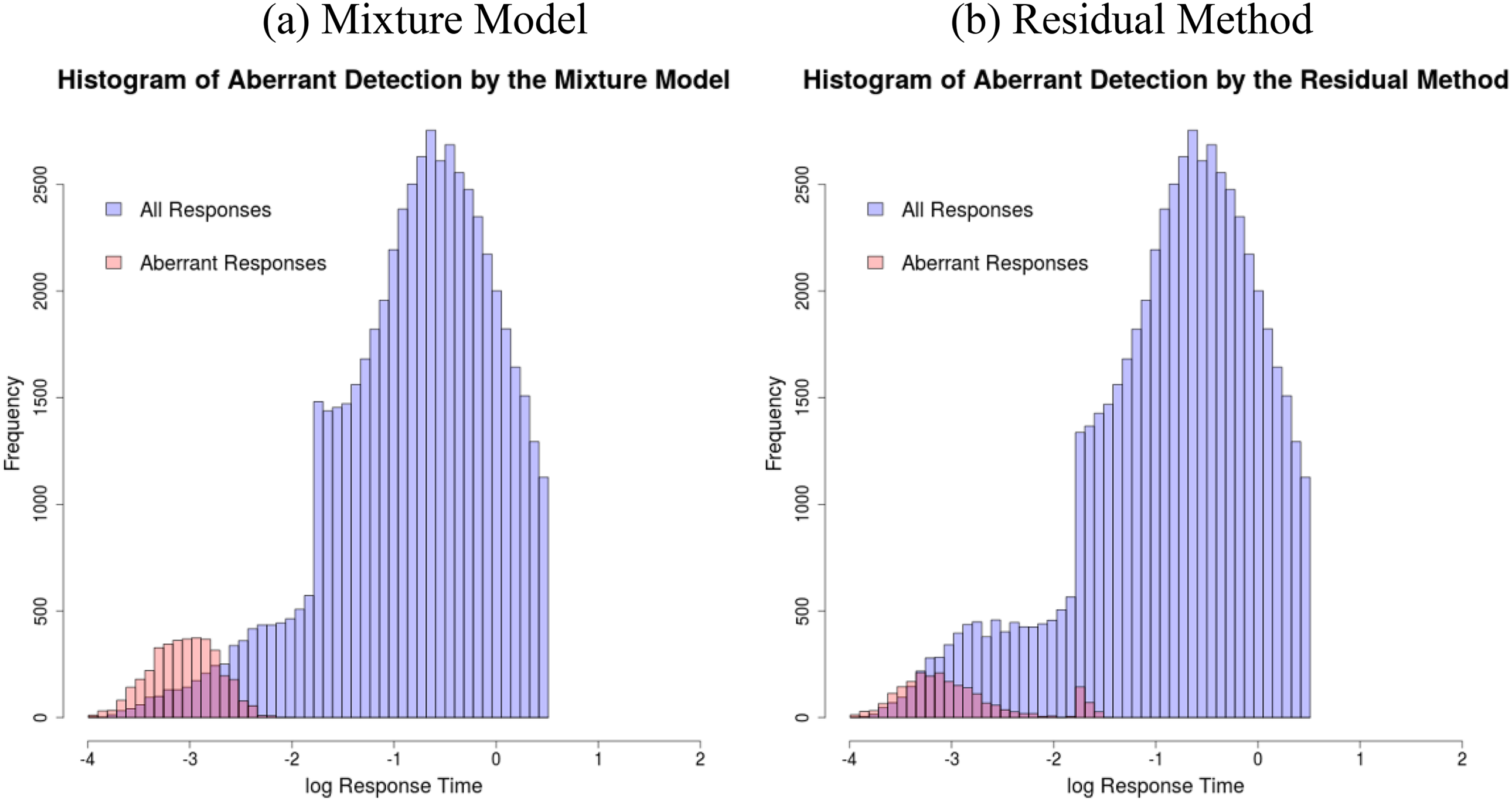
Histogram of log-response time classified by two behaviors (Real Data Example 1).

Figure 5.

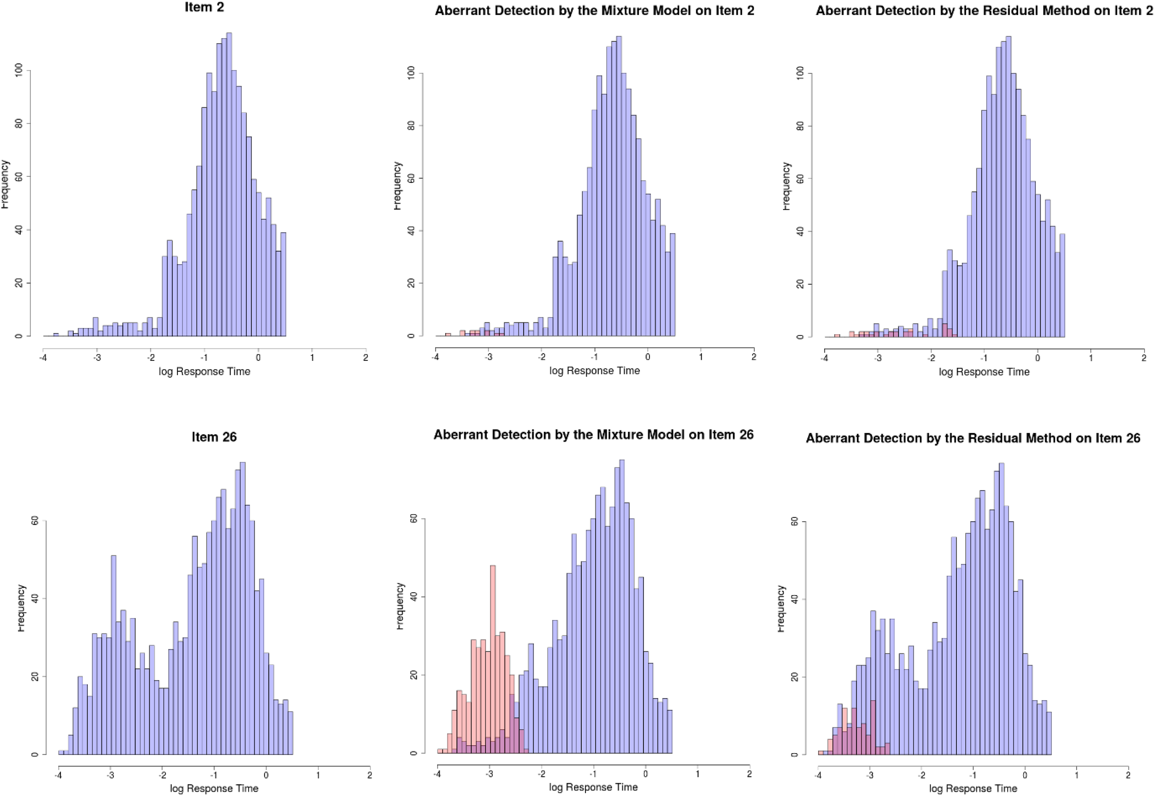
Histogram of item-level log-response time classified by two behaviors (Real Data Example 1).

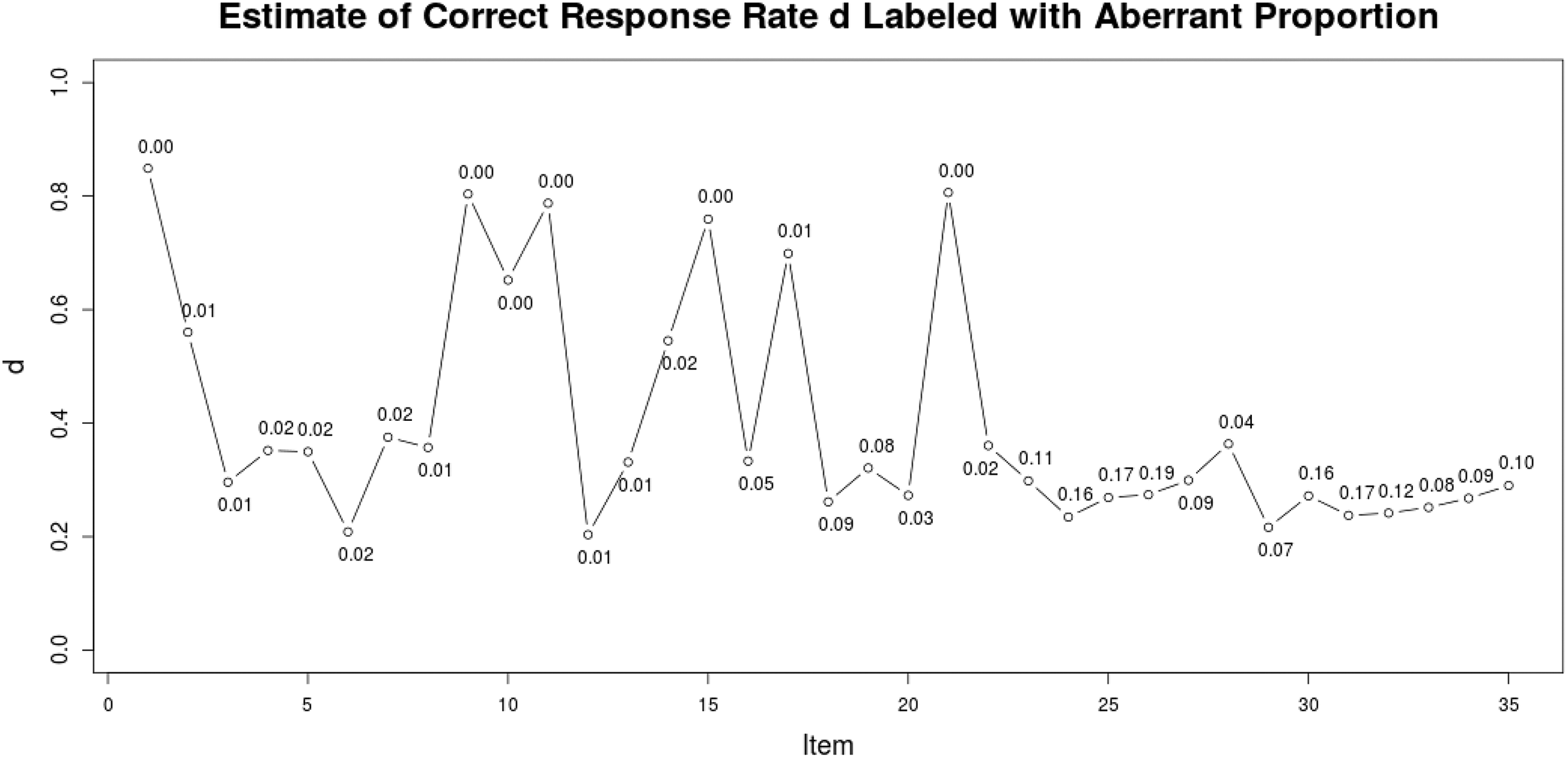
To further identify the specific type of aberrant behavior, Figure 6 presents the estimated ${\hat{d}}_{j}$ , for each item in the test, labeled by the proportion of aberrant behavior on the respective item. As reflected in Figure 6, items positioned in the second half of the test (e.g., Items 24–35) show higher proportion of aberrance, and their estimated ${\hat{d}}_{j}$ s are close to the chance value of 0.2∼0.25. This observation indicates that the aberrant behavior is likely the rapid guessing behavior that leads to aberrantly short RTs. However, further analysis need to be conducted to verify such a conclusion because using d_j alone is not enough to differentiate rapid guessing from cheating.

Figure 6.

Estimated correct response rate for the aberrant behavior for each item, labeled by the proportion of aberrant behavior on the respective item (Real Data Example 1).

5.2. A High-Stakes Computerized Adaptive Testing Example

This data set comes from a large-scale, high-stakes, computerized adaptive test. The item bank consists of 620 multiple choice items, and examinees’ responses are recorded as either right or wrong. Examinee sample size is 2,106. Test length is 37 and testing time is 75 minutes. Due to the adaptive design, every item is answered by a different set of examinees, and the examinee sample size per item varies between 5 and 364. RT distribution of all item-by-person encounters again reveals a bimodal structure, which implies that the examinees are from a mixture of two populations with potentially different behaviors. Even though this is a high-stakes test, the data come from well-protected testing sites, and the items used for this data collection are secure items. Hence, we expect the aberrant behavior mainly takes the form of rapid guessing rather than cheating. Similar to the previous example, both mixture hierarchical model and nonmixture model were fitted to this data set, and the Markov chain length is 50,000 with the first 10,000 as burn-in. The DIC from mixture model is 281,399, whereas the DIC from nonmixture model is 616,367. Again, mixture model exhibits better fit. For the mixture model, ${\hat{µ}}_{β} = 0.474$ and ${\hat{σ}}_{β}^{2} = .209$ , and for the nonmixture model, ${\hat{µ}}_{β} = 0.415$ and ${\hat{σ}}_{β}^{2} = .246$ . As in the first real data example, the response time is reported using the minute unit.

Figure 7 presents the histogram of log RTs classified as from solution and aberrant behaviors. Mixture model method flagged 1,194 aberrant behaviors (i.e., 1.52% of aberrance) from 336 examinees, whereas residual method flagged 10,118 behaviors (i.e., 13.1% of aberrance) from 1,967 examinees. As shown in Figure 7, many of the cases flagged by the residual method do not have extremely short RTs; in fact, those observed log-RTs are between −1 and 0 (i.e., 22–60 seconds), which can hardly be considered as “rapid” guessing. In this regard, we suspect that those behaviors flagged solely by residual method are false detection. One possible explanation is that in the residual method, the cutoff of the Bayesian posterior predictive p value determines the number of false alarms in case there is no irregular responding. Hence, a more stringent cutoff (i.e., lower than typical .05) might help lower the false alarm rate.

Figure 7.

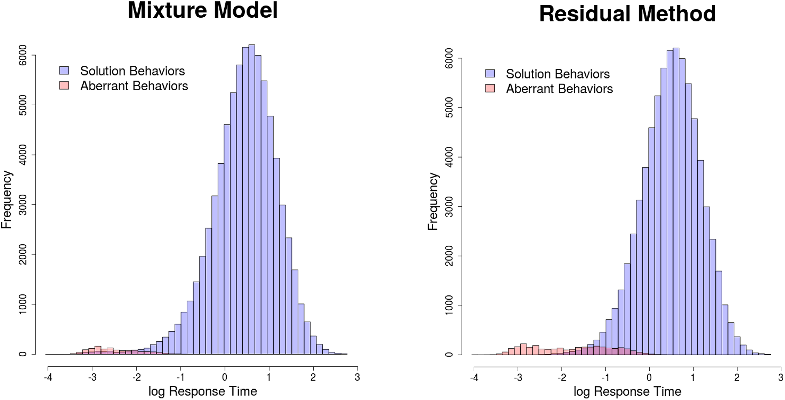
Histogram of log-response time classified by two behaviors (Real Data Example 2).

To further verify our conjecture, we plotted the box plot of the estimated $\hat{τ}$ s for examinees diagnosed with aberrant behaviors from both methods in Figure 8. As indicated in the figure, the average estimated $\hat{τ}$ s from residual method are much higher and also vary widely across examinees diagnosed with aberrant behavior. On the other hand, the estimated $\hat{τ}$ s from the mixture model are much lower, which is in line with the hypothesis that examinees with lower speed tend to rush through toward the end of the test. Therefore, the results from mixture model are more reasonable than that of the residual method.

Figure 8.

Boxplot of estimated $\hat{τ}$ for persons diagnosed with aberrant behavior from two methods in Real Data Example 2.

6. Discussion

Online testing or web-based assessment is becoming a mainstream form of modern testing due to the internet’s flexibility, accessibility, and potential capacities for faster data analysis and reporting. In web-based standardized testing, RT can be recorded conjointly with the corresponding responses. This broadens the scope of potential modeling approaches because RTs can be analyzed in addition to analyzing the responses themselves. One appealing application of RT is to help distinguish aberrant behavior from normal behavior and to help diagnose problematic items. From psychometrics perspective, failing to recognize the existence of different behaviors can be detrimental to the validity of inferences based on the test scores. Moreover, the existence of compromised items in the test may also inflate the test score and result in invalid inferences.

Looking into the literature, most statistical analysis to identify aberrant behavior or item compromise belongs to the broader class of residual analysis or outlier detection (e.g., van der Linden & Guo, 2008; van der Linden & van Krimpen-Stoop, 2003; Wang, Shu, Shang, & Xu, 2015; Wise, 2017). This class of methods is flexible as they make no assumptions concerning the form of irregular behavior. However, it has low power if a large proportion of examinees exhibit aberrant behavior, as demonstrated in both the simulation studies. The performance of this class of methods could potentially be improved by employing an iterative purifying approach. That is, one refits the model repetitively using a “cleansed” data set after removing the aberrant responses/RTs. This approach is worth exploring in future studies. In this article, we introduce a mixture hierarchical model to account for the dependency between item responses and item RTs with a special focus on differentiating between normal and aberrant behavior. The mixture model also offers an indicator showing the severity of item compromise (i.e., π_j ). This indicator effectively distinguishes compromised items from secure items in virtually all manipulated conditions, whereas the Bayesian residual method has heavy reliance on the severity of aberrance. The latter leads to low power and sometimes high false detection rate when the aberrance severity is high. While previous papers either focus on person-fit analysis or item fit analysis and those focus on item fit analysis have either rarely considered item misfit due to item compromise or have not included RT information, our article combines both objectives together to demonstrate that the mixture model approach offers checks on both items and persons.

The successful execution of the proposed mixture model approach requires using sophisticated model calibration algorithm. Different from the Monte Carlo expectation-maximization (MCEM) algorithm used in Wang and Xu (2015), we used the fully Bayesian MCMC algorithm. There are several reasons for making this choice. First, MCMC allows natural incorporation of certain prior information about the model parameters into the estimation processes. Second, it is relatively more straightforward than MCEM for complex models. Third, we can obtain the entire posterior distribution of each parameter from MCMC rather than just the point estimate. Therefore, statistical inference on certain parameters can be carried out easily if necessary. The details of the algorithm are provided in the Online Appendix, and the R code is available from the authors. Alternatively, the comprehensive prior information and initial values presented in the previous sections enable readers to try out this model using other available Bayesian packages.

We acknowledge that this article is limited in a few aspects. First, the response time is assumed to follow lognormal distributions throughout this article, and a wrongly specified RT distribution will greatly deteriorate the performance of any model-based approach. However, one flexibility of the hierarchical model, as well as its mixture extension, is that any model can be plugged in to model RT distribution. It does not have to be lognormal model, but it can be exponential, gamma, or even semiparametric models. Second, the current approach cannot differentiate rapid guessing and cheating for each item and person encounter, unless these two aberrant behaviors result in different RT distributions. In this case, a three-class mixture model would be ideal. However, from our real data example (see, e.g., Figure 4 or Figure 5 for item-level RT distributions), the majority of the item-level RT distributions exhibit a two-mode shape rather than a three-mode shape, implying that based on RT, only a two-class mixture model will be identified. At the very least, the objective of this article is to differentiate aberrant behavior from normal behavior, instead of differentiating cheating behavior from rapid guessing behavior. This latter objective is hard to achieve at person-by-item level without separation of RT information. At the item level, in practice, if we know certain items are likely to be compromised (e.g., being active for a long period), then we can restrain the prior of d_j to a certain range accordingly to speed up its convergence. Even so, using d_j alone is not sufficient to identify the specific type of aberrant behavior, future research needs to delve into this challenge further. Third, a well-recognized issue with mixture modeling approach is that if the difference between regular and irregular behavior is small, mixture model might not perform well (e.g., Depaoli, 2013; Tolvanen, 2008). Fourth, in the case of rapid guessing, the mixture model can be further extended to include the dependency of the type of behavior on elapsed testing time.

In closing, the aforementioned limitations need to be weighed against the potential advantages of the proposed mixture model approach, as exemplified in the simulation studies. Even though preventing aberrant behavior by carefully proctoring exams, enlarging item bank, increasing testing time, and increasing the number of parallel forms are commendable—prevention is better than cure—given that writing and calibrating new items are extremely expensive, routinely analyzing responses/RTs to diagnose any possible aberrant behavior and item compromise still has profound practical value. Last but not least, detection of aberrant behavior (especially cheating behavior) is sensitive in reality, so instead of merely relying on statistical evidence, careful qualitative analyses of the entire RT pattern for flagged test takers and items and corroborating evidence such as reported irregularities during the testing session should also be taken into consideration. Overall, we present an improved and efficient method for detecting aberrant behavior during testing that would also permit precise identification of compromised items.

Supplemental Material

Supplemental Material, DS_10.3102_1076998618767123 - Detecting Aberrant Behavior and Item Preknowledge: A Comparison of Mixture Modeling Method and Residual Method

Supplemental Material, DS_10.3102_1076998618767123 for Detecting Aberrant Behavior and Item Preknowledge: A Comparison of Mixture Modeling Method and Residual Method by Chun Wang, Gongjun Xu, Zhuoran Shang, and Nathan Kuncel in Journal of Educational and Behavioral Statistics

Footnotes

Declaration of Conflicting Interests

The author(s) declared no potential conflicts of interest with respect to the research, authorship, and/or publication of this article.

Funding

The author(s) disclosed receipt of the following financial support for the research, authorship, and/or publication of this article: This research is partially supported by 2014 CTB/McGraw-Hill R&D research grant and Institute of Education Sciences grant R305D160010.

Notes

References

Bolt

D. M.

Cohen

A. S.

Wollack

J. A

. (2002). Item parameter estimation under conditions of test speededness: Application of a mixture Rasch model with ordinal constraints. Journal of Educational Measurement, 39, 331–348.

Boughton

K. A.

Yamamoto

. (2007). A HYBRID model for test speededness. In von Davier

Carstensen

C. H.

. (Eds.), Multivariate and mixture distribution Rasch models (pp. 147–156). New York, NY: Springer.

Chang

Y. W.

Tsai

R. C.

Hsu

N. J.

(2014). A speeded item response model: Leave the harder till later. Psychometrika, 79, 255–274.

Cizek

G. J.

(1999). Cheating on tests: How to do it, detect it, and prevent it. New York, NY: Routledge.

Dean

Martineau

(2012). A state perspective on enhancing assessment and accountability systems through systematic implementation of technology. In Lissitz

R. W.

Jiao

(Eds.), Computers and their impact on state assessment: Recent history and predictions for the future (pp. 55–77). Charlotte, NC: Information Age.

Depaoli

(2013). Mixture class recovery in GMM under varying degrees of class separation: Frequentist versus Bayesian estimation. Psychological Methods, 18, 186–219.

Fan

Wang

Chang

H.-H.

Douglas

(2012). Utilizing response time distributions for item selection in CAT. Journal of Educational and Behavioral Statistics, 37, 655–670.

Karabatsos

(2003). Comparing the aberrant response detection performance of thirty-six person-fit statistics. Applied Measurement in Education, 16, 277–298.

Lievens

Chapman

D. S.

(2009). Recruitment and selection. In Wilkinson

Redman

Snell

Bacon

(Eds.), The SAGE handbook of human resource management (pp. 133–154). London, England: Sage.

10.

Marianti

Fox

G. J. A.

Avetisyan

Veldkamp

B. P.

Tijmstra

. (2014). Testing for aberrant behavior in response time modeling. Journal of Educational and Behavioral Statistics, 39, 426–451. doi:10.3102/1076998614559412

11.

McLeod

L. D.

Lewis

(1999). Detecting item memorization in the CAT environment. Applied Psychological Measurement, 23, 147–160.

12.

Meijer

R. R.

Sijtsma

(1995). Detection of aberrant item score patterns: A review of recent developments. Applied Measurement in Education, 8, 261–272.

13.

Meijer

R. R.

Sijtsma

(2001). Methodology review: Evaluating person fit. Applied Psychological Measurement, 25, 107–135.

14.

Meyer

J. P.

(2010). A mixture Rasch model with item response time components. Applied Psychological Measurement, 34, 521–538.

15.

Qian

Staniewska

Reckase

Woo

(2016). Using response time to detect item preknowledge in computer-based licensure examinations. Educational Measurement: Issues and Practice, 35, 38–47.

16.

Ranger

(2013). A note on the hierarchical model for responses and response times in tests of van der Linden (2007). Psychometrika, 78, 538–544.

17.

Rouder

J. N.

Sun

Speckman

P. L.

Zhou

(2003). A hierarchical Bayesian statistical framework for response time distributions. Psychometrika, 68, 589–606.

18.

Sackett

P. R.

Lievens

(2008). Personnel selection. Annual Review of Psychology, 59, 419–450.

19.

Schnipke

D. L.

Scrams

D. J.

(1997). Modeling response times with a two-state mixture model: A new method of measuring speededness. Journal of Educational Measurement, 34, 213–232.

20.

Tolvanen

(2008). Latent growth mixture modeling: A simulation study (Unpublished doctoral dissertation). University of Jyväskylä, Jyväskylä, Finland.

21.

van der Linden

W. J.

(2007). A hierarchical framework for modeling speed and accuracy on test items. Psychometrika, 72, 287–308.

22.

van der Linden

W. J.

Entink

R. H. K.

Fox

J.-P.

(2010). IRT parameter estimation with response times as collateral information. Applied Psychological Measurement, 34, 327–347.

23.

van der Linden

W. J.

Guo

(2008). Bayesian procedures for identifying aberrant response-time patterns in adaptive testing. Psychometrika, 73, 365–384.

24.

van der Linden

W. J.

van Krimpen-Stoop

E. M.

(2003). Using response times to detect aberrant responses in computerized adaptive testing. Psychometrika, 68, 251–265.

25.

van Krimpen-Stoop

E. M.

Meijer

R. R

. (2000). Detecting person misfit in adaptive testing using statistical process control techniques. In van der Linden

W. J.

Glas

C. A. W.

(Eds.), Computerized adaptive testing: Theory and practice (pp. 211–219). Norwell, MA: Kluwer Academic.

26.

Wang

Chang

H. H.

Douglas

J. A.

(2013a). The linear transformation model with frailties for the analysis of item response times. British Journal of Mathematical and Statistical Psychology, 66, 144–168.

27.

Wang

Fan

Chang

H.-H.

Douglas

J. A.

(2013b). A semiparametric model for jointly analyzing response times and accuracy in computerized testing. Journal of Educational and Behavioral Statistics, 38, 381–417.

28.

Wang

Shu

Shang

(2015). Assessing item-level fit for the DINA model. Applied Psychological Measurement, 39, 525–538.

29.

Wang

(2015). A mixture hierarchical model for response times and response accuracy. British Journal of Mathematical and Statistical Psychology, 68, 456–477.

30.

Wang

Zheng

Chang

H.-H.

(2014). Does standard deviation matter? Using “standard deviation” to quantify security of multistage testing. Psychometrika, 79, 154–174.

31.

Wise

S. L

. (2017). Rapid-guessing behavior: Its identification, interpretation, and implications. Educational Measurement: Issues and Practice. doi:10.1111/emip.12165

32.

Wise

S. L.

DeMars

C. E.

(2006). An application of item response time: The effort-moderated IRT model. Journal of Educational Measurement, 43, 19–38.

33.

Wise

S. L.

Kong

(2005). Response time effort: A new measure of examinee motivation in computer-based tests. Applied Measurement in Education, 18, 163–183.

34.

Yang

(2007). Methods of identifying individual guessers from item response data. Educational and Psychological Measurement, 67, 745–764.

Supplementary Material

Please find the following supplemental material available below.

For Open Access articles published under a Creative Commons License, all supplemental material carries the same license as the article it is associated with.

For non-Open Access articles published, all supplemental material carries a non-exclusive license, and permission requests for re-use of supplemental material or any part of supplemental material shall be sent directly to the copyright owner as specified in the copyright notice associated with the article.

0.00 MB

0.19 MB