Does the Package Matter? A Comparison of Five Common Multilevel Modeling Software Packages

Abstract

This study compared five common multilevel software packages via Monte Carlo simulation: HLM 7, Mplus 7.4, R (lme4 V1.1-12), Stata 14.1, and SAS 9.4 to determine how the programs differ in estimation accuracy and speed, as well as convergence, when modeling multiple randomly varying slopes of different magnitudes. Simulated data included population variance estimates, which were zero or near zero for two of the five random slopes. Generally, when yielding admissible solutions, all five software packages produced comparable and reasonably unbiased parameter estimates. However, noticeable differences among the five packages arose in terms of speed, convergence rates, and the production of standard errors for random effects, especially when the variances of these effects were zero in the population. The results of this study suggest that applied researchers should carefully consider which random effects they wish to include in their models. In addition, nonconvergence rates vary across packages, and models that fail to converge in one package may converge in another.

Keywords

multilevel modeling statistical software Monte Carlo simulation

As accessibility to data in the educational and social sciences has improved and the burden of statistical computation has diminished, researchers have increasingly adopted multilevel modeling techniques to analyze clustered or dependent data. Many statistical software packages are available for multilevel modeling, and they differ in terms of ease of use, cost, speed, and comprehensiveness.

Although some literature discusses multilevel packages in isolation (i.e., Bates et al., 2016), the literature provides very little guidance on selecting a software package. Palardy’s (2011) review of HLM 7 implicitly noted differences across software programs when he commented that HLM exhibited better rates of convergence, as compared to other (unnamed) multilevel programs. He observed that in some (unidentified) programs, “non-convergence is not uncommon when working with models that have a complex error structure (e.g., cross-classified model), little variance on one or more random effect, or linear dependence among random effects” (Palardy, 2011, p. 516).

The most comprehensive research study comparing the performance of multilevel software (Kreft, deLeeuw, & van der Leeden, 1994) evaluated five multilevel software packages. However, more than 20 years have elapsed since the publication of their work, and the landscape of multilevel software packages is vastly different today. In fact, only two of the packages from the original 1994 review have survived in some format: HLM and MLwiN (previously ML3). Moreover, the HLM software package uses a different estimation algorithm than it did in 1994, rendering much of the information in the article obsolete.

Several more-recent, nonpublished technical guides compare certain features, output, and results of various multilevel modeling packages. For instance, Albright and Marinova (2010) released an unpublished tutorial online for running multilevel models in SPSS, Stata, SAS, and R, using examples from the High School and Beyond (HSB) data set referenced in Raudenbush, Bryk, Cheong, and Congdon (2004). Albright and Marinova include background information regarding the terminology, notation, and general logic of multilevel analysis, and they present syntax and results from each software package for running unconditional, random-intercepts, and random-slopes models. However, their manuscript does not provide explicit comparisons of computational speed or efficiency across the four packages nor does it systematically compare the multilevel packages using multiple data sets.

Similarly, the Division of Statistics and Scientific Computation at the University of Texas at Austin (UT Austin, 2012) compared the results and estimation procedures of multilevel analyses conducted in SAS, Stata, HLM, R, SPSS, and Mplus, using the popular.csv data set from chapter 2 of Hox’s (2010) textbook. This article provided syntax and results for six models, which ranged in complexity from an unconditional model to one with a random intercept and slope with a cross-level interaction between Level-1 and Level-2 factors. SAS did not produce standard errors or p values for variance components that were very close to zero. In addition, both Stata and SPSS were unable to estimate the most complex model, which included two cross-level interactions (UT Austin, 2012).

These two unpublished manuscripts (Albright & Marinova, 2010; UT Austin, 2012) contributed important insights regarding differences across software in terms of input/syntax, output/results, production of standard errors and p values, convergence of complex models, and so on. However, both papers fit models using only one empirical data set. Hence, the idiosyncratic features of the chosen data set may have influenced their findings, which diminishes the generalizability of their results. Also, use of a single data set precluded the authors from assessing and comparing parameter estimation accuracy across software programs. Because they did not know the true parameter values underlying the data, they could not identify the degree of discrepancy between the model estimates and their corresponding true values. Further, neither manuscript explicitly compared the speed or efficiency of the various multilevel packages.

In contrast, Austin (2010) conducted a series of Monte Carlo simulations to compare the performance of various estimation procedures for fitting multilevel logistic regression models as a function of the number of clusters and the size of the clusters. Austin (2010) did not address software computational speed but focused on estimation accuracy, revealing that multilevel packages did perform differently from one another when estimating multilevel logistic models. However, the estimation algorithms used to fit multilevel logistic models are quite different from those used for multilevel linear models (MLMs).

Anecdotally, we had also observed differences across various multilevel software packages, in terms of program speed and convergence rates, especially when fitting random coefficient models with one or more near-zero random slope variances. Given that no recently published papers provide a comprehensive, detailed comparison of the different software packages with respect to their performance in difficult modeling contexts, Palardy’s (2011) assertions and our experiences with multilevel software programs motivated us to systematically compare the performance of five common multilevel software packages. We were especially interested in comparing their performance when fitting multilevel models when one or more of the randomly varying slopes has a population variance of 0.

From Data to Inferences

Generally speaking, observations that are clustered tend to exhibit some degree of interdependence: Observations that are nested within one cluster tend to be more similar to each other in terms of an outcome variable than two observations that are drawn from two different clusters. This interdependence, which is a result of the sampling design (the nesting of observations within clusters), affects the variance of the outcome, which in turn affects the estimates of the standard errors. In such a scenario, making the assumption of independence produces incorrect standard errors: The estimates of the standard errors are smaller than they should be. Therefore, the Type I error rate is inflated for all inferential statistical tests that make the assumption of independence. Multilevel analyses explicitly estimate and model the degree of relatedness of observations within the same cluster, thereby correctly estimating the standard errors and eliminating the problem of inflated Type I error rates.

When modeling multilevel data, it is crucial to select (a) the appropriate statistical model that captures the nature of the data, (b) a suitable estimation theory or strategy that allows us to make appropriate inferences about our data, and (c) the computational algorithm, which implements the estimation theory in practice (Raudenbush & Bryk, 2002). The distinction between the estimation theory (e.g., full maximum likelihood [FML]) and the computational algorithm is critical: It explains why two software packages that fit the same models using the same estimation strategy (FML) could perform differently. Different packages may use the same default estimation strategy (maximum likelihood [ML] or restricted maximum likelihood [RML]) but may employ different computational algorithms and/or starting values (Garson, 2013; Raudenbush & Bryk, 2002).

Statistical Model

Statistical models are made up of a system of equations that connect the response (i.e., dependent) variable to the explanatory (i.e., independent) variable(s). The MLM provides an avenue to partition the variance of the dependent variable into within and between cluster components. The simplest MLM model, the random effects analysis of variance, allows the intercept to randomly vary across clusters: This between-cluster variance component is represented by τ₀₀. The system of equations representing this model is

Y_{i j} = β_{0 j} + e_{i j}; e_{i j} \sim N (0, σ^{2}),

β_{0 j} = γ_{00} + u_{0 j}; u_{0 j} \sim N (0, τ_{00}) .

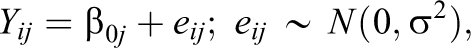
Here, β_0j is a random coefficient and is comprised of a fixed and a random component (i.e., β_0j ∼ N[γ₀₀, τ₀₀]). For instance, the estimated mean for cluster j is a linear combination of the expected score γ₀₀ (i.e., the fixed component) and organization j’s deviation, u_0j (i.e., the random component), from the expected score. τ₀₀ represents the between-cluster variability around γ₀₀. Partitioning the variance into within-cluster variance and between-cluster variance enables more appropriate computation of the standard errors. Within-cluster predictors may explain within-cluster variance, thereby reducing σ², whereas between-cluster variables may reduce τ₀₀. The latter of the two corresponds to an intercept-as-outcomes model (Raudenbush & Bryk, 2002).

When additional within-cluster predictors are included in the model, the effects of these variables can randomly vary across clusters. To do so requires an additional random coefficient, β_1j, which allows the effect of the predictor (X1) on the dependent variable to randomly vary in the population (i.e., across observed clusters). The average effect of X1 on Y is γ₁₀ (i.e., the fixed component) and cluster j’s deviation from this average is u _1j (i.e., the random component). This level-specific equation is represented by $β_{1 j} = γ_{10} \times X 1 + u_{1 j}; u_{1 j} \sim N (0, τ_{11})$ . The slopes-as-outcomes model includes contextual effects (i.e., W1, cluster-level covariates) to explain the between-cluster variability of Level-1 slopes (i.e., explaining τ₁₁; Raudenbush & Bryk, 2002). This level-specific equation is $β_{1 j} = γ_{10} \times X 1 + γ_{11} \times W 1 + u_{1 j}; u_{1 j} \sim N (0, τ_{11})$ .

A model with p explanatory effects is stored in a column vector, Γ (Gamma), with p + 1 rows; whereas the variance components at the cluster level are stored in a square matrix, Τ (Tau), whose dimension is determined by the number of random effects, r. When only the diagonal elements are estimated (i.e., $τ_{00} {: τ}_{rr}$ ), this corresponds to a variance components model in which all between-cluster random effects are assumed to be uncorrelated, and Τ is a diagonal matrix. When the off-diagonal elements are also estimated ( $τ_{10} = τ_{01}$ ), Τ is said to be unstructured, and Τ contains r unique variances and [(r × r + 1)/2 − r] unique covariances. The assumption of homogeneous within-cluster variances is typically utilized in organizational MLM models resulting in the estimation of a sole within-cluster variance component, σ². However, this assumption can be relaxed, and Hedeker has extended the standard mixed model to allow for the within-cluster variance component to randomly vary across clusters (Hedeker & Nordgren, 2013). However, models that allow for heterogeneous Level-1 variances are beyond the scope of the study at hand. All models in the current study estimated an unstructured Τ and a sole within-cluster variance component, σ².

Estimation Theory

Estimation theory guides the estimation of parameters using data. Generally, fixed effects at Level-2 are estimated using generalized least squares. Packages typically estimate randomly varying Level-1 coefficients with empirical Bayes, which uses a weighted combination of OLS and predicted Level-2 values (Woltman, Feldstain, MacKay, & Rocchi, 2012). The most common estimation techniques for estimating variance components are FML and RML. The goal of ML estimation is to find the parameter values that maximize the likelihood of observing the data. FML chooses estimates of Γ, Τ, and σ² “that maximize the joint likelihood of these parameters for a fixed value of the sample data, Y” (Raudenbush & Bryk, 2002, p. 52). In contrast, RML maximizes the joint likelihood of Τ and σ² given the observed sample data, Y. Thus, when estimating the variance components, RML takes the uncertainty due to loss of degrees of freedom from estimating fixed parameters into account, while FML does not (Raudenbush & Bryk, 2002; Snijders & Bosker, 2011). Therefore, FML tends to underestimate variance components, particularly with small numbers of clusters. However, to compare models using the RML deviance, the fixed effects structures must be identical; model comparisons with differing fixed and random effects should utilize the deviance provided by FML (McCoach & Black, 2008; Snijders & Bosker, 2011).

Computational Algorithms

In multilevel models involving random coefficients, closed-form solutions are generally not available. Therefore, to approximate the solution, parameter estimates are updated iteratively, and they converge upon a solution when the change in the log-likelihood is smaller than some threshold (i.e., convergence criterion) using a specific computational method or algorithm. Both FML and RML may use one of the several iterative computational algorithms, each differs in terms of the speed and reliability of convergence (Raudenbush & Bryk, 2002). Some of the most common computational procedures for executing ML approaches in a multilevel framework include expectation maximization (EM), Newton–Raphson (NR), and Fisher scoring (Raudenbush & Bryk, 2002; Swaminathan & Rogers, 2008; West, Welch, & Galecki, 2015). It is differences in these computational algorithms across packages that lead to differences in the performance of different multilevel packages. For instance, the default estimation technique in both HLM and SAS is RML; however, differences emerge with respect to the computational algorithms that they employ by default. Specifically, HLM uses the EM algorithm and Fisher scoring in combination, whereas SAS uses ridge-stabilized NR and Fisher scoring (Garson, 2013; West et al., 2015). Hence, software packages may produce discrepant results, even when using the same estimation technique (i.e., RML or FML) due to their use of different computational algorithms. The differences are most likely to manifest themselves when estimating challenging models (Hox, 2010; Raudenbush & Bryk, 2002, p. 437). Common estimation methods can be broken into three categories: (a) brute-force methods such as the EM algorithm, (b) gradient-based methods such as NR and Fisher scoring, and (c) Quasi-Newton methods such as bound optimization by quadratic approximation (BOBYQA; Powell, 2009), where differences surface with respect to the second derivative of the log-likelihood of the model, the Hessian Matrix (Skrondal & Rabe-Hesketh, 2004).

Brute Force

EM

The EM algorithm views estimation as a missing data problem. In an iterative fashion, the algorithm alternates between an expectation (E) step, in which the statistical package evaluates the log-likelihood of the model using current parameter estimates, followed by a maximization (M) step, in which the program updates the estimates to values that maximize the log-likelihood. The model converges when the change in log-likelihood between the current and previous iteration is smaller than some predefined criterion and guarantees the solution is at some local maximum. However, because the estimated information matrix is not inherently available, the sampling distribution of the ML estimates is not known (i.e., standard errors are not asymptotic). Many modeling packages utilize the EM algorithm because its computations are fairly easy and generally converge on an admissible solution (Raudenbush & Bryk, 2002). However, EM is not always the fastest choice and can converge slowly, especially “when the likelihood is flat, meaning that there exists substantial uncertainty about the parameters given the data” (Raudenbush & Bryk, 2002, p. 444).

Gradient

Gradient-based methods require the partial second derivatives (i.e., the Hessian) to be solved in some manner; therefore, these methods are more computationally demanding relative to the EM algorithm. Although more computationally demanding per iteration, these methods can converge in fewer iterations than EM, especially given good starting values. If the system to be solved is quadratic, it is possible for these methods to converge in a single iteration. A benefit to these methods is that asymptotic standard errors of the solution are available. However, these methods do rely on good starting values.

NR

The NR algorithm is one of the most commonly used techniques for determining MLM solutions (West et al., 2015). Initially, a first-order Taylor series is expanded at the models current parameter estimates and solves both the gradient and the Hessian matrices such that the solution equals zero, thus producing updated parameter estimates. Therefore, this method inherently utilizes the observed Hessian matrix. It is for this reason the NR method can converge in a single iteration. However, if the system to be solved is ill conditioned (i.e., log-likelihood is not concave), computation time for each iteration will increase without providing a substantially better solution. If the variance–covariance matrix is semipositive-definite, the solution for variance component might be outside the acceptable range (i.e., producing negative variances, representing Heywood cases).

Fisher scoring

Similar to the NR method, a first-order Taylor series is expanded at the current parameter estimate values; however, instead of solving the Hessian matrix, it is estimated. Specifically, the negative of the expected Hessian matrix—known as Fisher’s information—is utilized when solving for zero. This difference is not to be taken lightly, as it eases the computational burden by eliminating the need to solve the Hessian matrix (deLeeuw & Meier, 2008). Another benefit to the FS method is that the solution is positive-definite, thus avoiding Heywood cases.

Quasi-Newton

These methods are characterized by the fact that only the first-order derivatives—the gradient—must be solved, whereas the Hessian is approximated in some manner. The use of an approximated Hessian matrix greatly reduces the computational burden.

BOBYQA

The BOBYQA (Powell, 2009) algorithm is a Quasi-Newton approach to estimation that is implemented in the lme4 package.

Software packages may harness the respective strengths of each of these algorithms, and most packages use a combination of algorithms to execute ML techniques. The EM algorithm often begins the estimation process to generate starting values, given the relative computational ease of the algorithm. Then packages may switch from EM to gradient-based methods once they have generated good starting values for the parameter estimates.

Statistical Software Packages

In this study, we compared five common software packages for multilevel modeling: HLM 7 (hlm2.exe), Mplus 7.4 (mplus.exe), R (lme4 V1.1-12; lmer), Stata 14.1 (mixed command), and SAS 9.4 (PROC MIXED). When choosing a software program, important considerations are (a) ease of use (i.e., reading data in and specifying models), (b) flexibility with respect to estimation techniques and methods, (c) how model convergence issues are handled, (d) ease at which the Level-2 deviates (i.e., u _0j) can be accessed, and (e) the degree of difficulty to run simulations and save output over replications. With respect to the latter, interested readers can consult Online Appendix for detailed information on how to run simulations for each of these programs.

Table 1 contains an overview of the default estimation techniques and methods utilized by each statistical software, as well as the default treatment of Τ, the variance–covariance matrix of random effects (e.g., between cluster variance components).

Table 1.

Default Estimation Across Software Programs

Software Program	SAS	HLM 7	Mplus	Stata	R {lme4}
Procedure/function	PROC MIXED	hlm2.exe	mplus.exe	mixed command	lmer()
Technique	RML	RML	FML	FML	RML
Method/algorithm	NR	EM with FS	Accelerated EM	EM followed by NR	BOBYQA
Enhancement	Ridge stabilized	None	Quasi-Newton with FS	None	Quadratic approximation
T	Diagonal	Unstructured	Diagonal	Diagonal	Unstructured
Significance of T	Z	χ²	t	Z	N/A
Store random effects	Yes	Yes	No	Yes	Yes
Operating system	Cross-platform	Windows	Cross-platform	Cross-platform	Cross-platform

Note. BOBYQA = bound optimization by quadratic approximation; RML = restricted maximum likelihood; FML = full maximum likelihood; EM = expectation maximization.

HLM 7

HLM by Scientific Software International (Version 7; Raudenbush, Bryk, Cheong, Congdon, & Du Toit, 2011; Scientific Software International, 2014) has been commercially available since 1991. HLM 7 was released in 2011 (Palardy, 2011) and HLM 7.01 in 2013.

Ease of use

HLM allows users to read data, specify models, and estimate these models, all within a user-friendly graphical user interface (GUI). To estimate MLM models, it is necessary to create a multivariate data matrix file, in which Level-1 and Level-2 identification variables are selected, as are level-specific variables. Using the GUI, users select the dependent variable, within-level predictors, and select which of these effects randomly vary across Level-2 units. All independent variables can be automatically centered with respect to the grand mean or the group mean, prior to estimating the model. As effects are modeled, the reduced form equation is populated in the GUI. By default, Τ is an unstructured matrix; therefore, all off-diagonal parameters are estimated.

Estimation options

HLM provides several different estimation techniques for the variance–covariance components, including RML (the default for two-level models) and FML. In terms of estimation methods, HLM uses a combination of the EM algorithm and Fisher scoring to compute the estimates (Raudenbush & Bryk, 2002). By default, Fisher scoring is utilized every fifth iteration but repeats the iteration using EM if it does not meet the predetermined criteria. With regard to estimating the fixed effects, HLM uses empirical Bayes to compute an optimally weighted estimate using OLS for Level-1 coefficients and a generalized least squared estimate for Level-2 coefficients (Raudenbush & Bryk, 2002; Woltman et al., 2012).

By default, HLM uses a total of 100 iterations and determines convergence using a criterion of 10⁻⁶; however, the user can easily change within the GUI.

Convergence issues

By default, HLM performs an “automatic fix-up” strategy when the solution for Τ is inadmissible, specifically, the correlations between errors to their expected parameter space to improve convergence (Palardy, 2011); thus, in an ad hoc fashion, a bounded strategy on the parameter space is conducted and no estimation warnings are issued to the user.

Random effects

HLM is capable of producing the empirical Bayes estimates for all randomly varying effects (e.g., u _0j). These values are written out to a text file. This is not done by default.

Simulating

Estimating replicated data sets in HLM is not a user-friendly task, as it requires knowledge of programming (i.e., Windows Batch Language). This is because HLM provides no built in capability of doing so. More details on simulating in HLM can be found in Online Appendix.

Mplus 7.4

Mplus is a general latent variable modeling software program capable of estimating a variety of multilevel and latent variable models “within a fully integrated general latent variable modeling framework” (Muthén & Muthén, 2015).

Ease of use

Mplus requires basic data files that are free of column names. The input file (e.g., NAMES ARE) in the VARIABLE command specifies the variable names. Such a task can prove to be tedious as the number of variables increase; however, resources such as the R package MplusAutomation (Hallquist & Wiley, 2016) ease this task (among others). Within the VARIABLE command, users must specify variables that are measured at the within and between level as well as those that are measured at both levels.

Estimation options

With respect to estimation techniques, Mplus is limited to FML. For MLM, Mplus uses an accelerated EM algorithm which calls on both Quasi-Newton and Fisher scoring to optimize the function (Muthén & Muthén, 2012). By default, Mplus produces robust standard errors via a sandwich estimator.

Convergence issues

In the event, the objective function cannot be optimized using the Quasi-Newton and Fisher scoring steps, no parameter estimates are printed; however, if the matrix is not positive definite, a warning is offered. The TECH8 output (which must be requested) identifies the offending element.

Random effects

At this time, there is no out-of-the box method to request the empirical Bayes estimates of the randomly varying intercepts and slopes; rather, one must have a background in latent variable modeling. Specifically, the user must generate a phantom variable and regress the Level-2 random effects on this phantom variable and then save the factor scores in a delimited file.

Simulating

Using the MONTECARLO command, users can conduct full-scale simulations using a single input file. Both internal and external MonteCarlo simulation studies are available in Mplus.

lme4

The lme4 (for linear mixed effects) package in R (Bates et al., 2016) is currently on Version 1.1-15. Its primary functions are lmer (for fitting linear models), glmer (for generalized linear models), and nlmer (for nonlinear models; Bates, Mächler, Bolker, & Walker, 2015).

Ease of use

To estimate MLM models using the lme4 package, the user must possess at least a rudimentary understanding of the R language. Models are specified using a reduced form equation, and interaction terms can be generated at the time of estimation using the “*” operator. Because R is an object-oriented language, all model information is stored in a user-named object and can easily be accessed. Users can do any data preprocessing and postestimation processing in the R environment.

Estimation options

Both FML and RML (the default) are available in lmer. In terms of the computational algorithms, lmer utilizes Powell’s (2009) BOBYQA by default, while offering other optimizers to estimate Τ.

Convergence issues

The lmer function issues estimation warnings on a regular basis, thus placing the onus on the user. Due to the nature of BOBYQA, estimation is sensitive to the scaling of the parameters. To scale the estimated gradient at the estimate appropriately, lme4 scales gradients by the inverse Cholesky factor of the Hessian. The latter approach is used in the current version of lme4. The disadvantage of this approach is that it requires estimation of the Hessian (https://cran.r-project.org/web/packages/lme4/lme4.pdf, p. 15). The lmer community suggests testing alternate estimation methods available such as the Nelder–Mead simplex algorithm (Nelder & Mead, 1965).

Random effects

The ranef function: uj <- ranef(modObject) stores all empirical Bayes estimates of the randomly varying coefficients in the object “uj.”

Simulating

Executing replications in R is straightforward for users with knowledge of the R environment and complex data structures (e.g., list objects). Simulations can be executed using for loops, in which a parameter is incremented by some step value, or more efficiently using the lapply function. A user can define a function that will execute the model and store the pertinent information (e.g., parameter estimates, standard errors, and convergence status) into data objects.

Stata 14 (Version 14.1)

Stata is a general statistics software program (StataCorp, 2015a, 2015c). For MLMs, the mixed command is available and can handle various types of multilevel data structures, including two-level, three-level, and cross-classified models (StataCorp, 2015b). Additionally, Stata contains commands tailored for generalized linear and nonlinear multilevel models (StataCorp, 2015b).

Ease of use

Multilevel models are specified using a reduced form equation. By default, Stata assumes a diagonal Τ matrix for models with randomly varying slope coefficients (i.e., the random effects are not correlated). However, a variety of covariance structures can be requested (StataCorp, 2015b).

Estimation options

The default estimation technique is FML; however, RML estimation is also available. The mixed command uses the EM algorithm to generate starting values before switching to the NR algorithm for the remainder of the task. The mixed command also provides Quasi-Newton methods. When RML is employed, users can request small sample adjustments such as Kenward–Roger and Sattertherwaite approximation (StataCorp, 2015b).

Convergence issues

In the event the model does not converge, Stata will print warnings at each iteration indicating the log-likelihood is “not concave” and encourages users to specify the difficult option; however, this does not guarantee convergence. Alternatively, users can request to use only the EM algorithm or to use some combination of algorithms (StataCorp, 2015b).

Random effects

After estimation, the mixed postestimation command can be utilized to create new variables corresponding to the empirical Bayes estimates of the random intercepts and slopes.

Simulating

Replications can be executed with ease using the simulate command available in Stata. The command requires the user to program their custom routine in accordance with Stata’s syntax and allows users to specify the number of replications to be executed and what model information to save over replications.

SAS (Version 9.4)

SAS is a general purpose statistical program, capable of estimating both linear and nonlinear random effect models (SAS Institute Inc., 2013). The present study utilized the mixed procedure (PROC MIXED), which is the most common method for fitting linear random effect models (i.e., MLM) in SAS.

Ease of use

Preprocessing such as data manipulation and recoding (e.g., group/grand mean centering) can be done via a DATA step. MLM models are specified using a reduced form equation and automatically model an intercept; however, all randomly varying effects must be specified in the random command, including the intercept.

Estimation options

SAS offers a variety of estimation techniques such as FML, RML, and minimum variance quadratic unbiased estimators (MIVQUE0, Goodnight, 1978) for model estimation. When FML or RML is invoked, MIVQUE0 is used to determine the starting values. To carry out estimation, MIXED employs a ridge-stabilized NR algorithm to arrive at a solution set. MIXED also allows adjustments such as Kenward–Roger correction and/or Satterthwaite approximated degrees of freedom. However, this option is not available if an asymptotic method for estimating the variance–covariance matrix of the fixed effects is utilized (e.g., sandwich estimator). When utilizing this option, all standard errors are approximated based on the expected Hessian matrix (SAS Institute Inc., 2009).

Convergence issues

In the event the model does not converge, it is recommended to utilize the SCORING option that invokes Fisher scoring along with the default ridge-stabilized NR algorithm.

Random effects

Level-2 deviates (e.g., u _0j) can be requested using the output delivery system (ODS) option by specifying the appropriate ODS table name (e.g., SolutionR). All model details (e.g., parameter estimates and estimation details) can be stored in this manner.

Simulating

Analysts can utilize either the interactive matrix language (PROC IML) or SAS macros for simulations. The benefit of utilizing PROC IML lies in its ability to utilize an incremental parameter (i.e., the same estimation routine can be executed on hundreds of replicated data sets in a few short lines; however, when programming in PROC IML, the same routines (e.g., PROC MIXED) are not readily available, rather such an estimation routine must be user-programmed. On the other hand, utilizing macros affords all of the computational capabilities of SAS procedures; however, it is not as straightforward to increment a routine through simulated data sets. Model estimates are saved into a temporary file and ultimately are appended to a permanent data set via PROC APPEND.

The Current Study

Prior benchmarking studies have compared the computational speed and efficiency of statistical packages to help researchers make informed decisions about choosing software that suits their needs (e.g., Keeling & Pavur, 2007; Li & Lomax, 2011; Odeh, Featherstone, & Bergtold, 2010). However, no current studies include systematic investigations of whether and how various multilevel modeling packages differ with respect to accuracy, efficiency, and convergence when estimating MLMs. To address this gap in the statistical software literature, the current study compares the performance of five of the most commonly utilized software options for multilevel modeling: HLM, Mplus, R (lme4), Stata, and SAS. Specifically, we examined differences across packages in terms of speed, rates of convergence/admissibility, and parameter estimate recovery. Furthermore, we examined whether these differences vary as a function of the magnitude of the unique elements of Τ (i.e., τ₄₄ and τ₅₅), corresponding to variances in the Level-2 slopes for β₄ and β₅ across clusters, with a particular focus on how the software packages performed when the population values of selected variance components were zero.

We did not expect to see differences across programs in terms of fixed effect estimates. However, based on our prior multilevel modeling experiences, we hypothesized that more generalized statistical packages (i.e., Stata) might have difficulty estimating models that include multiple randomly varying slopes, especially as the variance(s) for one or more of the slopes approach zero. Specifically, smaller variances produce flatter log-likelihood functions that are less able to differentiate the most likely parameter estimates (Enders, 2010). Consequently, statistical packages may run for a long time or fail to converge on a solution when estimating models with small variance components (Kenny, Kashy, & Cook, 2006). Given that EM can be especially slow to converge when the likelihood is flat (Raudenbush & Bryk, 2002), packages that rely more heavily on EM might be slower under such conditions. In NR, the calculation of the Hessian matrix is likely to become unstable when there is a ridge in the likelihood function and/or when the model contains a variance component that is near 0 (Stata, 2017). Therefore, we expected packages that rely more heavily on NR techniques to produce more nonconvergent solutions. In addition, in terms of estimation time, we expected to see differences across the software packages, and we hypothesized that more specialized modeling programs (i.e., HLM, Mplus) might be more time efficient.

Method

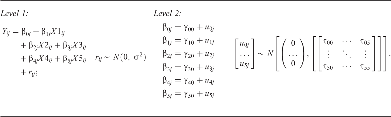
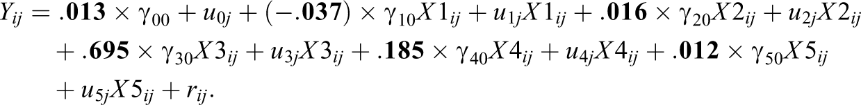
Simulation Model

The statistical model of interest was a two-level organizational hierarchical linear model containing a randomly varying intercept, along with five randomly varying slopes. The equations representing this statistical model appear below:

Level 1:		Level 2:
$Y_{i j} = β_{0 j} + β_{1 j} X 1_{i j} + β_{2 j} X 2_{i j} + β_{3 j} X 3_{i j} + β_{4 j} X 4_{i j} + β_{5 j} X 5_{i j} + r_{i j};$	$r_{i j} \sim N (0, σ^{2})$	$β_{0 j} = γ_{00} + u_{0 j}$ $β_{1 j} = γ_{10} + u_{1 j}$ $β_{2 j} = γ_{20} + u_{2 j}$ $β_{3 j} = γ_{30} + u_{3 j}$ $β_{4 j} = γ_{40} + u_{4 j}$ $β_{5 j} = γ_{50} + u_{5 j}$	$[\begin{matrix} u_{0 j} \\ \dots \\ u_{5 j} \end{matrix}] \sim N [(\begin{matrix} 0 \\ \dots \\ 0 \end{matrix}), [[\begin{matrix} τ_{00} & \dots & τ_{05} \\ ⋮ & ⋱ & ⋮ \\ τ_{50} & \dots & τ_{55} \end{matrix}]]] .$

Factors fixed across all simulation conditions included the estimation model, the majority of the model parameter population values, the Level-1 and Level-2 sample sizes, the estimation technique (FML), and the covariance structure of Τ, which was always specified to be unstructured, regardless of the program’s default. Varying simulation conditions included the magnitudes of two of the five slope variances and the software program. The simulation contained 15 models in which we varied the magnitudes of the variance components for the randomly varying slopes. We estimated those 15 conditions across all five software packages, for a total of 75 different conditions.

Simulation Conditions

Fixed conditions

Estimation model

The estimation model as well as the fixed-component population values remained constant across all simulation conditions. The reduced form of the simulation model appears below, with the fixed population parameters in bold:

Y_{i j} = . 013 \times γ_{00} + u_{0 j} + (- . 037) \times γ_{10} X 1_{i j} + u_{1 j} X 1_{i j} + . 016 \times γ_{20} X 2_{i j} + u_{2 j} X 2_{i j} + . 695 \times γ_{30} X 3_{i j} + u_{3 j} X 3_{i j} + . 185 \times γ_{40} X 4_{i j} + u_{4 j} X 4_{i j} + . 012 \times γ_{50} X 5_{i j} + u_{5 j} X 5_{i j} + r_{i j} .

We generated the random components from a normal distribution with means equal to 0. At the student level, $r_{i j} \sim N (0, σ_{r}^{2} = .046)$ , whereas the population values for diagonal elements of Τ were $u_{0 j} \sim N (0, τ_{00} = .0801)$ , $u_{1 j} \sim N (0, τ_{11} = .040)$ , $u_{2 j} \sim N (0, τ_{22} = .040)$ , and $u_{3 j} \sim N (0, τ_{33} = .040)$ , whereas the population values for τ₄₄ and τ₅₅ varied across our 15 simulation conditions and are reported below.

Across simulation conditions, the population value for σ² and τ₀₀ were on average .71 and .08, respectively, when estimating the random effects analysis of variance model, leading to an ICC of .101.

Sample size

The sample size was fixed; all conditions contained 50 clusters, each with 200 Level-1 responses, resulting in a total sample size of 10,000. The large sample sizes at each level ensured adequate power to detect between-cluster variability, conditioning on a sufficient amount of within-cluster information (Maas & Hox, 2005). The selected Level-1 and Level-2 sample sizes also exceeded recommendations specified in a recently published simulation study (Schoeneberger, 2016), investigating the impact of sample size and other design factors on nonpositive definite matrices, model convergence, Type I error rates, statistical power, relative bias in parameter estimates, and confidence interval widths and coverage in multilevel models with dichotomous outcomes. In Schoeneberger’s (2016) study, Level-1 and Level-2 sample sizes of at least 100 and 40, respectively, were sufficient to overcome the issue of nonpositive definite random effect covariance matrices. Therefore, by exceeding these recommendations, we hoped to minimize the impact of sample size on model nonconvergence rates.

Estimation technique

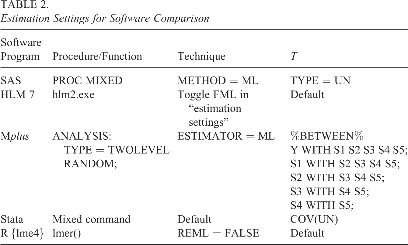
Due to Mplus’s inability to estimate multilevel models using RML, we estimated all models (across all programs) using FML. RML and FML estimation techniques yield nearly identical results with a large number of clusters. Given our explicit interest in measuring the divergence of the resulting parameter estimates from the specified true parameter values, it was important for the estimation method to remain consistent across statistical packages. For specific settings/syntax utilized for each of the five software programs, see Table 2.

Table 2.

Estimation Settings for Software Comparison

Software Program	Procedure/Function	Technique	T
SAS	PROC MIXED	METHOD = ML	TYPE = UN
HLM 7	hlm2.exe	Toggle FML in “estimation settings”	Default
Mplus	ANALYSIS: TYPE = TWOLEVEL RANDOM;	ESTIMATOR = ML	%BETWEEN% Y WITH S1 S2 S3 S4 S5; S1 WITH S2 S3 S4 S5; S2 WITH S3 S4 S5; S3 WITH S4 S5; S4 WITH S5;
Stata	Mixed command	Default	COV(UN)
R {lme4}	lmer()	REML = FALSE	Default

Computing

Because time was one of the major outcomes of interest, we executed all replications within each program on the same desktop computer. Therefore, all of the computer’s specifications were equivalent across programs, which was essential for our time comparisons.

Variable conditions

Statistical software

The statistical software packages used in this study included HLM 7, Mplus 7.4, R (lme4 1.1-5), Stata 14.1, and SAS 9.4. See Table 2 for statistical software options/arguments utilized in the simulation.

Variance component magnitude

We simulated the two slope variance components that varied over simulation conditions (e.g., τ₄₄ and τ₅₅) to be as small as zero and as large as .04 (shown in Table 3), where the latter matches the population values for τ₁₁ through τ₃₃.

Table 3.

Variance Component Sizes for Two Predictors (τ₄₄ and τ₅₅): .000, .001, .01, .02, and .04

Simulation Condition Number	τ ₄₄	τ ₅₅
1	.000	.000
2	.000	.001
3	.000	.010
4	.000	.020
5	.000	.040
6	.001	.001
7	.001	.010
8	.001	.020
9	.001	.040
10	.010	.010
11	.010	.020
12	.010	.040
13	.020	.020
14	.020	.040
15	.040	.040

The magnitude of these randomly varying population values was taken as the proportion of variance relative to the total variance estimated (e.g., $σ_{r}^{2} + τ_{00}$ ) from the random effect analysis of variance model, reported earlier. Therefore, population values of .04 corresponded to estimating a variance that was 95% smaller than the total estimated variance, .02 was 97.5% smaller, .01 was 98.8% smaller, .001 was 99.9% smaller, and .000 was 100% smaller. When considered as a proportion of the between-cluster variance in the intercept (τ₀₀), τ₁₁ through τ₃₃ were approximately half the size of τ₀₀, τ₄₄, or τ₅₅ of .02 is 75% smaller than τ₀₀, τ₄₄, or τ₅₅ of .01 is 87.5% smaller than τ₀₀ or τ₅₅, and .001 is 99% smaller than τ₀₀.

A variance component with a population parameter of zero represents the case in which a researcher specifies a slope as randomly varying, but the slope is essentially equal across the clusters in the population. We surmise that this is a fairly common occurrence.

Table 3 presents the 15 distinct simulation conditions that represent the combinations of these five possible variance component magnitudes for τ₄₄ and τ₅₅. These simulation conditions reflect only unique combinations, such that magnitudes of .010 for τ₄₄ and .020 for τ₅₅ were considered to be the same condition as .020 for τ₄₄ and .010 for τ₅₅. We executed 500 replications for each of the described 15 simulation conditions, across all software programs. Online Appendix contains specific details about running simulations in each of the statistical software programs.

Data Generation

Given the focus of the present study on comparing software programs, data generation needed to be independent of the programs used for model estimation. Therefore, we executed all data generation in the R environment (Version 3.3.0; The R Foundation, 2016) via a user-defined function that conformed to the linear mixed effects model (Laird & Ware, 1982) using the MASS package (Venables & Ripley, 2002):

y = X β + Z u + ϵ,

where the X matrix contains a column corresponding to the intercept as well as a column for each of the observed variables (e.g., X1, X2). These simulated data were drawn from the standard multivariate normal distribution using the mvrnorm function, assuming independence. β represents the vector of population values for the fixed effects, whereas the u matrix corresponds to the covariance matrix of the random effects and Z is the design matrix for the random effects. These random effects were assumed to be normally distributed around 0. The u matrix was generated by translating the covariance matrix into a correlation matrix, in which all off-diagonal estimates were set to .20, and was pre- and postmultiplied by the standard deviations of the random effects.

This afforded us the ability to generate β, as: β ∼ (Γ, Τ) across Level-2 units. We then created expected values by premultiplying B by X with respect to Level-2 membership. Within-level error was generated according to its population value, r_ij ∼ (0, σ²) and was added to the expected values, thus making the level-specific errors uncorrelated. Finally, we wrote a data frame to a local directory to conform to the varying data specification requirements per individual software programs.

Simulation Procedures

Automating estimation

For information on how we conducted the simulation across software programs, please see Online Appendix.

Masterfile creation

We combined all software-specific simulation results in R, creating a single data set that we indexed with a nominal code corresponding to the software program. To accomplish this task, we first compiled all results individually by software program. Afterward, we combined the matrices into one via the rbind function.

We were most interested in comparing the frequency with which each package was able to converge on a solution, the bias in parameter estimates and the analysis time. To address our research questions, we calculated several common statistics, including bias, relative bias for all parameter estimates (including fixed effects, variance components, and their standard errors) by condition and software package. Bias was computed as the difference between the parameter estimate of interest and its population, averaged across all replications. Relative bias expresses the degree of bias in a parameter by dividing the bias by the population parameter. Relative bias was computed as $\frac{\sum_{j = 1}^{n_{r}} (\frac{{(\hat{θ}}_{j} - θ)}{θ})}{n_{r}} \cdot 100$ , where θ is the true value of the parameter, ${\hat{θ}}_{j}$ is the parameter estimate of θ for replication j, and n_r is the number of replications (Bandalos & Leite, 2013). Therefore, relative bias of 5% means that the parameter estimate is 5% larger than its true population value. Convergence was computed as the percentage of replications in which the package produced an admissible solution. The proportion of inadmissible solutions was $\frac{n_{r} - n_{c}}{n_{r}}$ , where n_r represented the number of replications and n_c represented the number of convergent solutions. Time represented the total number of seconds it took the package to estimate a solution. These statistics were computed separately for each condition within each software package. We examined the average time for all replications (both convergent and nonconvergent) as well as the average amount of time for convergent and admissible solutions. As would be expected, the analyses with convergence issues were far slower than the analyses that converged and produced admissible solutions. We excluded all nonconvergent solutions from any analyses that compared the relative bias of the parameter estimates across software and conditions.

Results

Parameter Estimates

In general, when the programs converged and provided admissible solutions, the five packages provided nearly identical results for the fixed effects (Γ), the variance components (Τ and σ²), and the standard errors of the fixed effects. By design, lme4 does not produce standard errors for variance components, and Stata and SAS often had difficulty producing standard errors for variance components when the population value for the variance component was zero. However, when the programs produced standard errors for the variance components, the standard error estimates were also virtually identical across programs. Furthermore, in general, the parameter estimates exhibited very little bias. Traditionally, relative bias of less than 5% is considered fairly benign (Bandalos & Leite, 2013; Hoogland & Boomsma, 1998). None of the parameter estimates for the variance components exhibited relative bias of 5% or greater for any packages across all conditions. The parameter estimates for certain fixed effects (Γ) did exhibit a small amount of bias. Figures 1 through 4 depict the relative bias in γ₀ ₀, γ₁₀, γ₂ ₀, and γ₅ ₀ by software and condition. These four effects were the only parameter estimates for which at least one relative bias estimate exceeded the 5% threshold.

Figure 1.

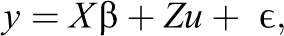
Relative bias for γ₀ ₀ by software and condition. Y-axis is the mean percentage relative bias across all 500 replications. The area within the dashed lines is generally considered to represent a nonproblematic degree of bias. Recall that Conditions 1–5 contain at least one variance component with a population value of 0; for more detailed information on conditions, consult Table 3.

Figure 2.

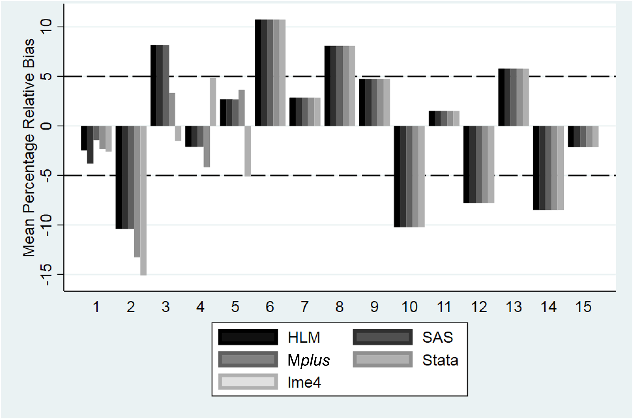
Relative bias in γ₁ ₀ by software and condition. Y-axis is the mean percentage relative bias across all 500 replications. The area within the dashed lines is generally considered to represent a nonproblematic degree of bias. Recall that Conditions 1–5 contain at least one variance component with a population value of 0; for more detailed information on conditions, consult Table 3.

Figure 3.

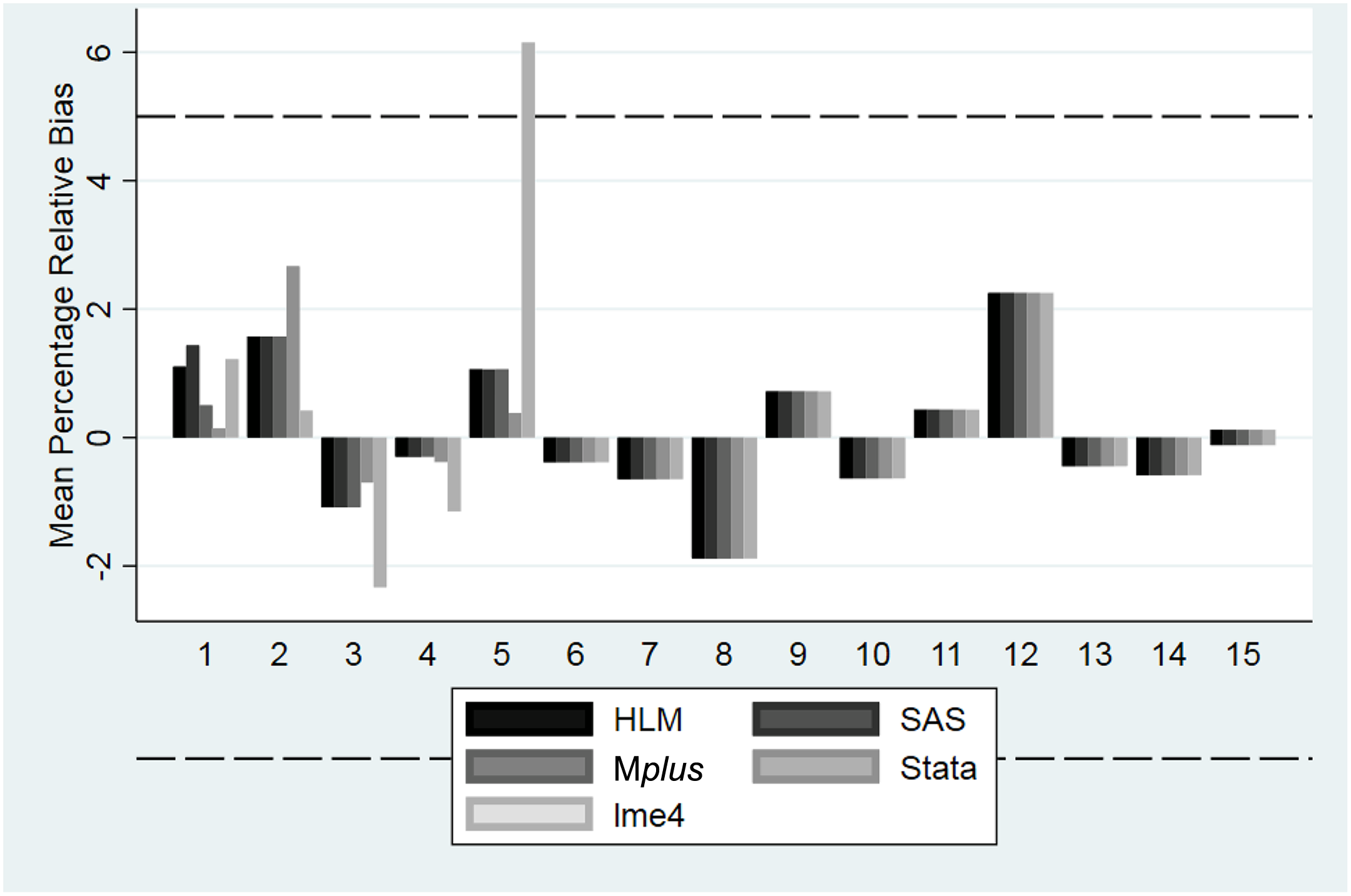
Relative bias in γ₂ ₀ by software and condition. Y-axis is the mean percentage relative bias across all 500 replications. The area within the dashed lines is generally considered to represent a nonproblematic degree of bias. Recall that Conditions 1–5 contain at least one variance component with a population value of 0; for more detailed information on conditions, consult Table 3.

Figure 4.

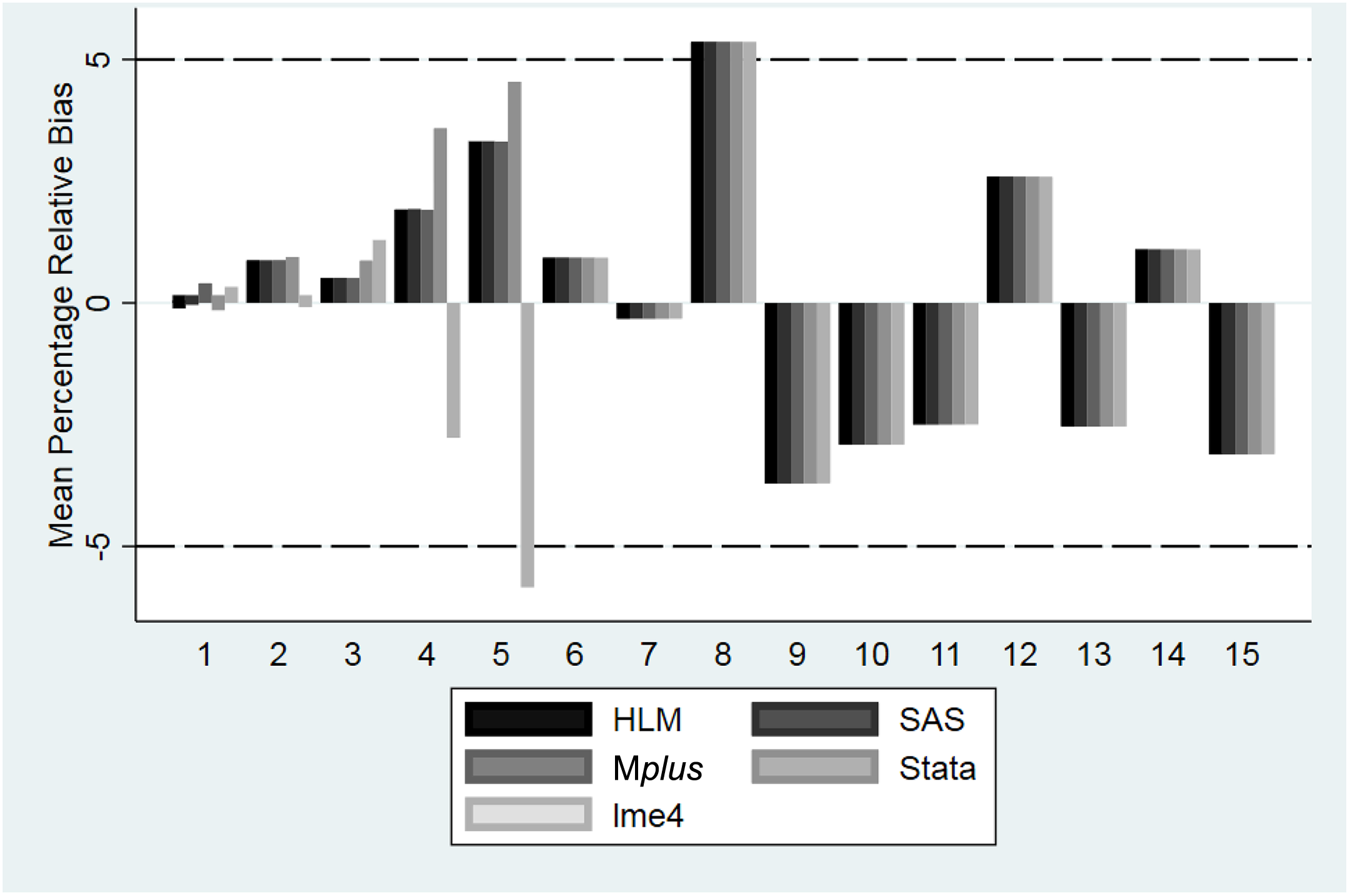
Relative bias in γ₅ ₀ by software and condition. Y-axis is the mean percentage relative bias across all 500 replications. The area within the dashed lines is generally considered to represent a nonproblematic degree of bias. Recall that Conditions 1–5 contain at least one variance component with a population value of 0; for more detailed information on conditions, consult Table 3.

The degree of bias was generally similar across software packages. One exception was the bias for γ₁₀ in Condition 5, which was substantially larger in lme4 than it was in any of the other software packages. In addition, in Conditions 4 and 5, the direction of the bias for γ₅₀ was negative in lme4 and positive in the other four software packages. However, when the software packages produce parameter estimates, they generally appear to be very similar.

Estimation Time

More interesting were the results comparing estimation times and rates of convergent/admissible solutions. With respect to the first five conditions, each of which contain at least one variance component that is 0 in the population; Figure 5 contains a boxplot of the estimation times by software package for all admissible solutions, whereas Figure 6 contains mean estimation times by software package for all replications, regardless of convergence status.

Figure 5.

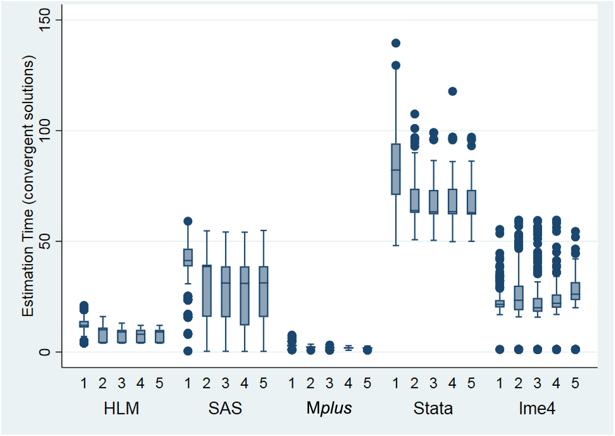
Comparison of estimation times among the five packages across the five conditions containing at least one variance component that is 0 in the population. Time is reported in seconds. Only admissible solutions are included in this graph.

Figure 6.

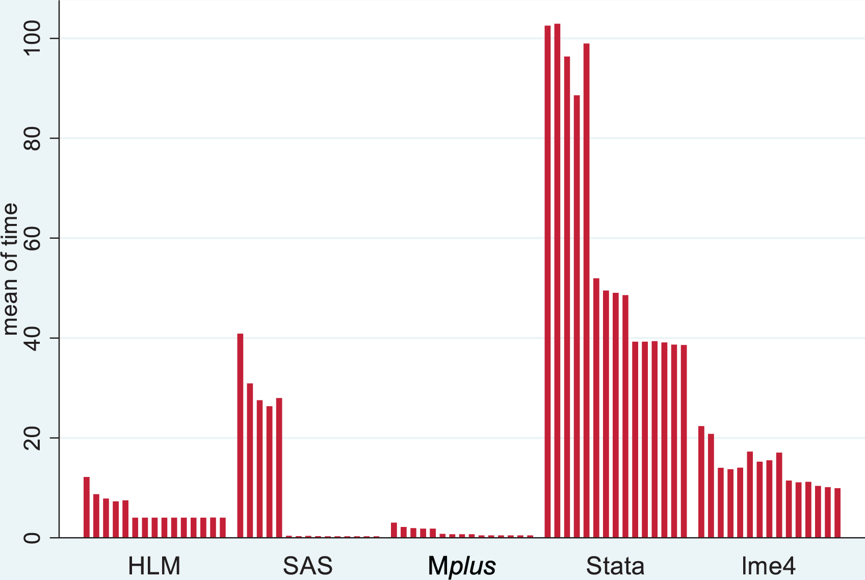
Estimation time for all solutions (both admissible and inadmissible) across Conditions 1–15.

Several trends emerged in terms of estimation time. First, estimation times were typically longer for Conditions 1 through 5, the conditions that contained at least one randomly varying slope that was zero in the population. Second, overall, Mplus was the fastest software program, and Stata was clearly the slowest. SAS was also very fast, except when estimating models which featured at least one variance component that was zero in the population (e.g., the first five simulation conditions). In these conditions, Mplus, HLM, and R had faster computational times than SAS. In fact, HLM was substantially faster than SAS in the first five conditions; however, SAS was faster than HLM when estimating models in which all population variance components were nonzero (i.e., Conditions 6–15). In these remaining 10 conditions, SAS and Mplus had the fastest computational speeds; SAS was actually slightly faster than Mplus. The estimation times were fairly uniform across all conditions for the R package, lme4:: lmer; however, lme4 was noticeably slower than HLM, Mplus, and SAS. More specifically, lme4 was always slower than Mplus and HLM, and the R package was faster than SAS when estimating models with population variance components of zero. However, SAS was faster than lme4 when estimating models with population variance components larger than zero.

Clearly, the five software packages differ in terms of estimation speed/efficiency, and inadmissible solutions generally appear to take more time than admissible ones. Mplus and HLM were noticeably and consistently faster than SAS, Stata, or lme4 across all conditions, and their speed advantage was even more pronounced for models that attempted to estimate at least one variance component that was 0 in the population.

Model Convergence

None of the software packages produced any inadmissible solutions for Conditions 6 through 15 in which all slopes had nonzero variance components in the population. Therefore, we focus on reporting results from Conditions 1 through 5, for which lme4 produced a troubling number of nonconvergent and error-laden solutions. For details on these problematic conditions by software package, see Table 4 (number of replications) and Figure 7 (proportion of replications). In fact, in Conditions 3 through 5, over 60% of the replications produced nonconvergence warnings; overall, across the first five conditions, almost half of the lme4’s replications warned of nonconvergence. In these conditions, the R package displayed three different types of error messages. The most common was a nonpositive definite Hessian matrix, which accounted for 53% of the lme4 error messages. Nonconvergence after reaching the maximum number of iterations accounted for 46% of the errors, and 1% of the lme4 messages labeled the results as “nearly unidentifiable” due to a large eigenvalue ratio. The fact that lme4 produced so many nonconvergence error messages in Conditions 1 through 5 was a striking finding. However, even though lme4 was plagued by these nonconvergent error messages, the program still produced parameter estimates. Also, despite the warning messages produced by R, lme4 did typically perform well; the parameter estimates generally did not differ from the parameter estimates for the convergent solutions. However, for the remainder of this article, we include only the fully convergent solutions in our software comparisons.

Table 4.

Nonconvergent and Problematic Replications by Software Package

Condition	HLM	Software	Package
Condition	HLM	Mplus	Stata	R (lme4)	Total
1	4	27	122	41	194
2	0	0	74	183	257
3	0	0	60	326	386
4	0	0	45	326	371
5	0	0	67	368	435
6–15	0	0	0	0	0
Total	4	27	368	1,244	1,643

Figure 7.

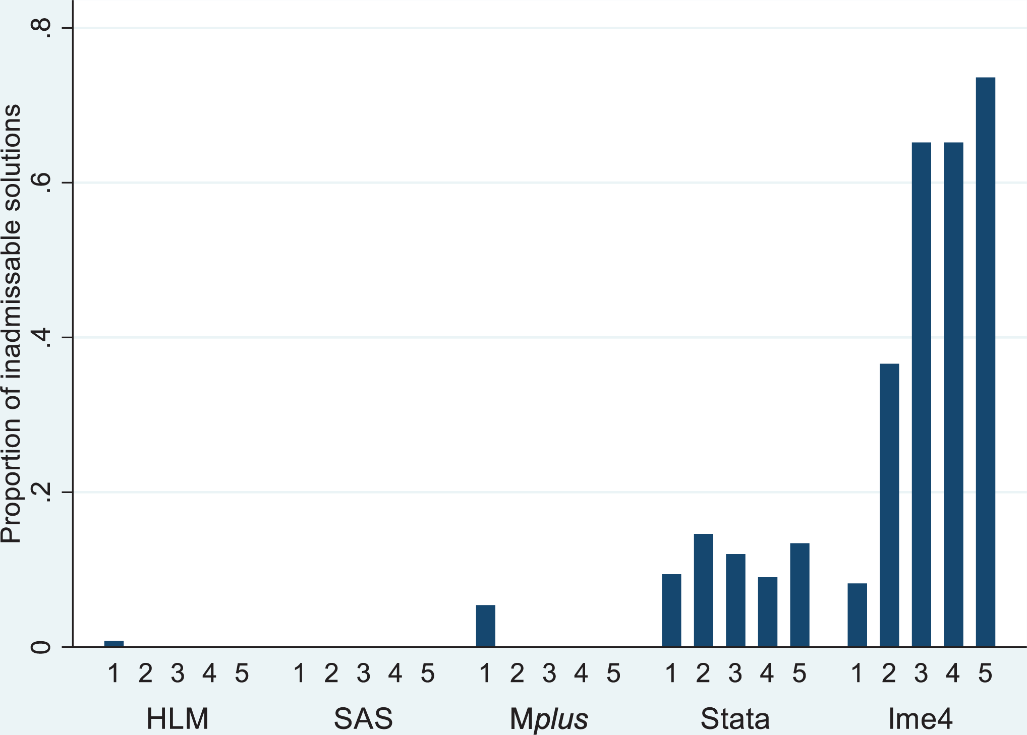
Proportion of inadmissible solutions (Conditions 1–5).

Stata also exhibited nonconvergence problems for 11.8% of the replications in Conditions 1 through 5. For these nonconvergent solutions, Stata displayed the fixed effects, random effects, and standard errors for the fixed effects but failed to display standard errors for any of the variance components. In addition, Stata failed to produce any parameter estimates at all for 75 replications in Condition 1 and one replication in Condition 2. Therefore, overall, 14.7% of the Stata replications in Conditions 1 through 5 were problematic. Again, we examined the nonconvergent solutions. Generally, the parameter estimates for the fixed effects and the variance components for the nonconvergent solutions were similar to those for the convergent solutions.

Finally, both SAS and Stata failed to produce standard errors at least 50% of the time for the variance component that was zero in the population (τ₄₄ and/or τ₅₅). Figure 8 shows the proportions of replications that were missing a standard error estimate for τ₄₄ (specified to be zero in the population) in Conditions 1 through 5. Recall that lme4 never reports standard error estimates for the variance components by design; therefore, we do not report rates of missingness for the standard errors in lme4 (which are 100% by design).

Figure 8.

Proportion of missing standard errors for τ₄₄ in Conditions 1–5 across the five software packages. Because lme4 does not produce standard errors for the variance components by design, it is excluded from this graph.

Discussion

Although all programs appear to produce very similar estimates for fixed effects, random effects, and standard errors for the fixed effects, the programs do differ in three ways: (a) convergence rates, (b) production of standard errors, and (c) computational speed.

Both R (lme4) and Stata had convergence issues when estimating models with at least one population variance component equal to zero. Although both programs produced error messages, the estimates of the fixed effects and the variance components appeared to adequately recover the population parameters. Mplus and HLM produced standard errors for the variance components more consistently than the other three software packages. However, both the utility of computing standard error estimates for the variance components and the best method for determining the statistical significance of the variance components are debatable. Raudenbush and Bryk (2002) question the utility of using the standard errors to evaluate the statistical significance of variance components. Variances cannot be negative; therefore, the sampling distribution of the variance estimates is skewed, especially under the null hypothesis (which is that the variance component is 0). “As a result, symmetrical confidence intervals and statistical tests based on these [standard errors] may be highly misleading” (Raudenbush & Bryk, 2002, p. 55). Instead, Raudenbush and Bryk advocate for the use of χ² tests to evaluate the statistical significance of the variance components, and the HLM software package reports these χ² tests by default. This is one of the unique features of the HLM program; none of the other software packages examined in this study provide χ² tests to evaluate the statistical significance of the variance components. Snijders and Bosker (2012) recommend using a modified likelihood ratio test to determine whether it is necessary to include variance components.

In terms of computational speed, Stata was by far the slowest of the software programs, and the difference was not trivial. In fact, on average (across all 15 conditions), Stata’s run times were over 3 times as long as those of lme4, approximately 5 times as long as those of SAS, over 9 times as long as those of HLM, and almost 50 times as long as those of Mplus. Such time differentials are not negligible, especially when estimating many large models with large data files or when conducting simulation studies. However, moving from a general-purpose statistical software such as SAS, Stata, or R into a more specialized program such as Mplus or HLM also comes at a cost in terms of the data analyst’s time. To use Mplus or HLM, the analyst must export the data and create a new data file; therefore, there is a time loss associated with the creation of the new data file and the transition into a new software package. In other words, even though Mplus and HLM were the fastest software packages for running the specified model, it may actually be slower to complete the analyses for smaller, less-complex models, after accounting for the amount of time that it takes to prepare and import the data into either HLM or Mplus.

However, if analysts seek to estimate larger, more complex models, it is possible that using a more-specialized software program could offer time savings overall. Additionally, if an analyst must estimate many models or is conducting simulations, specialized software may offer time advantages.

Additionally, differences between these programs in terms of ease in conducting simulation studies would also influence an analyst’s decision to choose one software package over another. By far, the most capable of the programs used in this study is lme4, as the functionality of the R environment offers tremendous flexibility with respect to carrying out simulation studies. However, this comes at a cost of computational time because the package does not directly pass the models to an executable file. Instead, information must pass through the R environment to the compiled lmer function.

Of the specialized software, Mplus is clearly the friendliest program for carrying out simulations. Mplus includes a Montecarlo command with which modelers can generate data for a given population model and estimate either the same applied model or an alternative model. HLM 7 is less flexible and requires knowledge of batch scripting to conduct simulations. Therefore, this software program is not particularly user-friendly for conducting such studies.

With respect to SAS, it is possible to use incremental variables for simulation work. However, analysts must use the IML procedure to do so. Unfortunately, the procedures available in SAS are not automatically available in IML, requiring users to program estimation routines at times from the ground up. Stata is also one of the more simulation friendly programs: It provides an avenue to manually program population values for models, generate data, estimate models, and pool results using the simulate command.

Limitations and Future Research

Although we considered five of the most common software packages, we did not include other possible programs/packages such as MLwiN, a specialty multilevel modeling program, or SPSS, a common general purpose software package. In addition, we only utilized one R package for this research, lme4, which appeared to be the most commonly used R package at the time of this study. However, we could have investigated additional R packages (e.g., nlme or xxM), which may have performed more efficiently than lme4.

The current study also used only one organizational model as the basis for its 15 simulation conditions. Different models may produce different results. Additionally, the most interesting differences among the software packages appear to occur when the specified model includes at least one variance component that is zero in the population. The present study only included two variance components with possible population parameter values equal to zero. Perhaps specifying the three remaining variance components in this organizational model with smaller near-zero (or zero) parameter values or three-level models with near-zero components at levels two and/or three could illuminate additional differences among these packages.

Given that Mplus does not have the ability to estimate multilevel models in RML, we used FML estimation for all software packages, which may appear as a limitation; however, we felt it necessary to accommodate for this limitation, due to the popularity of the software program. Generally speaking, the variance components did not exhibit substantial bias, and we would expect the fixed effect estimates to be virtually identical under RML and FML. However, given that RML is the preferred estimation method for multilevel models with small numbers of clusters, future researchers may wish to conduct similar comparisons across multiple software packages (other than Mplus) using RML to see whether the results differ across the two estimation strategies.

Finally, we generally used most of the default settings for the software programs because we were interested in comparisons of the software packages in their “native” form. However, it is certainly possible to increase the computational speed in any of these programs by providing good starting values or by changing the computational algorithm, if other options are available. For instance, future research could compare the performance of SAS when using the default NR to its performance when invoking SCORING=FISHER.

Also, in this study, we only examined models with normal outcomes. However, the major software packages may differ even more noticeably with regard to their estimation strategies for categorical, ordinal, and other nonnormal data. Future research should further compare the major multilevel software packages in terms of performance with logistic, ordinal, and count data as well as for other types of generalized linear models. Future research could also examine the performance of different software packages for more complex models with normal outcomes. These could include three-level models: cross-classified, random-effects models, and so on.

The utility of computing standard errors to evaluate the statistical significance is somewhat controversial. Future research should compare the performance of three commonly used methods to determine the necessity of a random effect: the χ² method used by HLM (Raudenbush & Bryk), Wald tests based on standard errors of the variance components, and the modified likelihood ratio tests of differences in the deviances of models with and without the variance components, as advocated by Snijders and Bosker (2010).

Finally, given the frequency with which R’s lme4 package (and to a lesser extent Stata) produced nonconvergence errors, future research should more systematically investigate the effects of such errors on bias and efficiency to help provide guidance about the gravity of the error messages. It would be beneficial to know whether such warning messages can safely be ignored and when they indicate underlying issues that bias the analytic results.

Our results demonstrated that there are major differences across the five software packages in terms of computational speed. This is critically important, particularly given that computing time may vary widely between software options as the number of random effects, cluster sizes, numbers of clusters, and overall sample sizes increase. Future research should systematically examine the effects of sample sizes (at Level 1 and Level 2), model complexity (both in terms of fixed and random effects), and other design features on the performance of these multilevel packages, especially in terms of computational speed.

Conclusion

Based upon the results of this study, it appears that all of the five software packages perform reasonably well, especially for models that do not attempt to estimate variance components that are 0 in the population. When they converged, all programs provided accurate estimates for fixed effects and variance components.

Therefore, determining the most appropriate software depends upon the priorities of the analyst. If time is a major concern, choose Mplus or HLM (or SAS, as long as the variance components are not actually zero). If convergence and admissibility are the main concerns, choose HLM, SAS, or Mplus. If it is important to obtain standard errors for the variances of the random effects, choose HLM or Mplus. In this, HLM has the added advantage of providing the χ² tests for the statistical significance of the variance components. Generally, specialized software programs (HLM and Mplus) do offer some advantages in terms of speed, convergence, and standard error estimation. However, these advantages come at a cost, in terms of both software price and the time that it takes to prepare and bring the data into an additional specialized software package.

This study also serves as a stark reminder that trying to estimate all possible slope coefficients as randomly varying is a problematic analytic strategy. Analysts should carefully consider whether each of the slopes in their multilevel model should be estimated as randomly varying, nonrandomly varying, or fixed before they begin estimating their models. Although it might seem tempting to allow all slopes to randomly vary, determine which random effects are unnecessary empirically, and then trim the unnecessary random effects from the model, this strategy is ill-advised. As demonstrated in this research, using such a strategy greatly increases the likelihood of obtaining a nonconvergent solution. If the analyst has fit a model with multiple randomly varying slopes, he or she has no clear way to determine which of the slopes should be eliminated from the multilevel model. Therefore, it is essential that analysts are judicious and parsimonious in their terms of which random slopes to include in their multilevel models. They should also be aware that models that fail to converge or are slow to converge are likely to contain one or more random effects that are near zero in the population. Unfortunately, such results may not provide guidance about which of the random effects needs to be eliminated.

We conclude with what is perhaps this study’s most important message: A model that fails to converge in one software package may actually produce an admissible solution in another software package or even by changing the estimation settings within the original software package. Therefore, researchers who have trouble running a complex model in one software package (and who have carefully considered which random effects to include and exclude a priori) should consider changing the defaults within the package or estimating the identical model in another software package before abandoning the model altogether.

Supplemental Material

Supplemental Material, DS_10.3102_1076998618776348 - Does the Package Matter? A Comparison of Five Common Multilevel Modeling Software Packages

Supplemental Material, DS_10.3102_1076998618776348 for Does the Package Matter? A Comparison of Five Common Multilevel Modeling Software Packages by D. Betsy McCoach, Graham G. Rifenbark, Sarah D. Newton, Xiaoran Li, Janice Kooken, Dani Yomtov, Anthony J. Gambino, and Aarti Bellara in Journal of Educational and Behavioral Statistics

Footnotes

Declaration of Conflicting Interests

The author(s) declared no potential conflicts of interest with respect to the research, authorship, and/or publication of this article.

Funding

The author(s) received no financial support for the research, authorship, and/or publication of this article.

ORCID iD

D. B. McCoach

References

Albright

J. J.

Marinova

D. M.

(2010). Estimating multilevel models using SPSS, Stata, SAS, and R. Retrieved from http://www.indiana.edu/∼statmath/stat/all/hlm/hlm.pdf

Austin

P. C.

(2010). Estimating multilevel logistic regression models when the number of clusters is low: A comparison of different statistical software procedures. The International Journal of Biostatistics, 6, 1–18. doi:10.2202/1557-4679.1195

Bandalos

Leite

(2013). Use of Monte Carlo simulation studies in Structural Equation Modeling research. In Hancock

Mueller

(Eds.), Structural equation modeling: A second course (2nd ed.) (pp. 625–666). Charlotte, NC: Information Age.

Bates

Mächler

Bolker

Walker

(2015). Fitting linear mixed-effects models using lme4. Journal of Statistical Software, 67, 1–48. doi:10.18637/jss.v067.i01

Bates

Mächler

Bolker

Walker

Christensen

R. H. B.

Singmann

… Green

(2016, 4 16). Linear mixed-effects models using “Eigen” and S4. Retrieved from https://cran.r-project.org/web/packages/lme4/lme4.pdf

deLeeuw

Meier

(2008). Introduction to Multilevel Analysis. In deLeeuw

Meier

(Eds.) Handbook of Multilevel Analysis (pp. 1–75). New York, NY: Springer.

Division of Statistics and Scientific Computation, University of Texas at Austin. (2012). Two-level hierarchical linear models using SAS, Stata, HLM, R, SPSS, and Mplus . Retrieved from https://stat.utexas.edu/images/SSC/Site/hlm_comparison-1.pdf

Enders

C. K.

(2010). Applied missing data analysis. New York, NY: Guilford.

Garson

G. D.

(2013). Hierarchical linear modeling: Guide and applications. Thousand Oaks, CA: Sage.

10.

Goodnight

(1978). Computing MIVQUE0 estimates of variance components. Cary, NC: SAS Institute.

11.

Hallquist

Wiley

(2016, 8 29). Automating Mplus model estimation and interpretation. Retrieved from https://cran.r-project.org/web/packages/MplusAutomation/MplusAutomation.pdf

12.

Hedeker

Nordgren

(2013). MIXREGLS: A program for mixed-effects location scale analysis. Journal of Statistical Software, 52(12), 1–38.

13.

Hoogland

J. J.

Boomsma

(1998). Robustness studies in covariance structure modeling: An overview and a meta-analysis. Sociological Methods and Research, 26, 329–367.

14.

Hox

J. J.

(2010). Multilevel analysis: Techniques and applications (2nd ed.). New York, NY: Routledge.

15.

Keeling

K. B.

Pavur

R. J.

(2007). A comparative study of the reliability of nine statistical software packages. Computational Statistics & Data Analysis, 51, 3811–3831. doi:10.1016/j.csda.2006.02.013

16.

Kenny

D. A.

Kashy

D. A.

Cook

W. L.

(2006). Dyadic data analysis. New York, NY: The Guilford Press.

17.

Kreft

I. G. G.

de Leeuw

van der Leeden

(1994). Review of five multilevel analysis programs: BMDP-5 V, GENMOD, HLM, ML3, VARCL. The American Statistician, 48, 324–335.

18.

Laird

N. M.

Ware

J. H.

(1982). Random-effects models for longitudinal data. Biometrics, 38, 963–974.

19.

Lomax

R. G.

(2011). Analysis of variance: What is your statistical software actually doing? The Journal of Experimental Education, 79, 279–294. doi:10.1080/00220973.2010.481684

20.

Maas

C. J. M.

Hox

J. J.

(2005). Sufficient sample sizes for multilevel modeling. Methodology, 1, 86–92. doi:10.1027/1614-1881.1.3.86

21.

McCoach

D. B.

Black

A. C.

(2008). Evaluation of model fit and adequacy. In O’Connell

A. A.

McCoach

D. B.

(Eds.), Multilevel modeling of educational data (pp. 245–272). Charlotte, NC: Information Age.

22.

Muthén

L. K.

Muthén

B. O.

(2012). Mplus user’s guide (7th ed.). Los Angeles, CA: Author.

23.

Muthén

B. O.

Muthén

L. K.

(2015). Mplus 7.4 Base Program and Combination Add-On [Computer software]. Retrieved from http://www.statmodel.com

24.

Nelder

J. A.

Mead

(1965). A simplex method for function minimization. The Computer Journal, 7, 308–313. doi:10.1093/comjnl/7.4.308

25.

Odeh

O. O.

Featherstone

A. M.

Bergtold

J. S.

(2010). Reliability of statistical software. American Journal of Agricultural Economics, 92, 1472–1489. doi:10.1093/ajae/aaq068

26.

Palardy

G. J.

(2011). Review of HLM 7. Social Science Quarterly Review, 29, 515–520.

27.

Powell

M. J. D.

(2009). The BOBYQA algorithm for bound constrained optimization without derivatives. Cambridge, England: Cambridge University’s Department of Applied Mathematics and Theoretical Physics.

28.

Raudenbush

S. W.

Bryk

A. S.

(2002). Hierarchical linear models: Applications and data analysis methods (2nd ed.). Thousand Oaks, CA: Sage.

29.

Raudenbush

S. W.

Bryk

A. S.

Cheong

Y. F.

Congdon

R. T.

(2004). HLM 6: Hierarchical linear and nonlinear modeling. Lincolnwood, IL: Scientific Software International.

30.

Raudenbush

S. W.

Bryk

A. S.

Cheong

Y. F.

Congdon

R.T.

du Toit

(2011). HLM7: Hierarchical linear and nonlinear modeling. Lincolnwood, IL: Scientific Software International.

31.

SAS Institute Inc. (2009). SAS/STAT 9.2 user’s guide, second edition. Cary, NC: Author.

32.

SAS Institute Inc. (2013). SAS 9.4 [Computer software]. Retrieved from https://www.sas.com/en_us/home.html

33.

Schoeneberger

J. A.

(2016). The impact of sample size and other factors when estimating multilevel logistic models. Journal of Experimental Education, 84, 373–397. doi:10.1080/00220973.2015.1027805

34.

Scientific Software International. (2014). HLM extractor executable: An HLM utility tool to extract columns from HLM 6 outputs [Computer software]. Lincolnwood, IL: Author.

35.

Skrondal

Rabe-Hesketh

(2004). Generalized latent variable modeling: Multilevel, longitudinal, and structural equation models. Boca Raton, FL: CRC Press.

36.

Snijders

T. A. B.

Bosker

R. J.

(2012). Multilevel analysis: An introduction to basic and advanced multilevel modeling (2nd ed.). London, England: Sage.

37.

StataCorp. (2015a). Stata base reference manual: Release 14. College Station, TX: Stata Press.

38.

StataCorp. (2015b). Stata multilevel mixed effects reference manual: Release 14. College Station, TX: Stata Press.

39.

StataCorp. (2015c). Stata statistical software: Release 14 [Computer software]. College Station, TX: StataCorp LP.

40.

Swaminathan

Rogers

H. J.

(2008). Estimation procedures for hierarchical linear models. In O’Connell

A. A.

McCoach

D. B.

(Eds.), Multilevel modeling of educational data (pp. 469–519). Charlotte, NC: Information Age.

41.

The R Foundation. (2016). The R Project for Statistical Computing [Computer software version 3.3.0]. Retrieved from https://www.R-project.org

42.

Venables

W. N.

Ripley

B. D.

(2002). Random and mixed effects. In Venables

W. N.

Ripley

B. D.

(Eds.), Modern Applied Statistics with S (4th ed., pp. 271–300). New York, NY: Springer Science+Business Media.

43.

West

B. T.

Welch

K. B.

Galecki

A. T.

(2015). Linear mixed models: A practical guide using statistical software (2nd ed.). Boca Raton, FL: CRC Press.

44.

Woltman

Feldstain

MacKay

J. C.

Rocchi

(2012). An introduction to hierarchical linear modeling. Tutorials in Quantitative Methods for Psychology, 8, 52–69. doi:10.20982/tqmp.08.1.p052

Supplementary Material

Please find the following supplemental material available below.

For Open Access articles published under a Creative Commons License, all supplemental material carries the same license as the article it is associated with.

For non-Open Access articles published, all supplemental material carries a non-exclusive license, and permission requests for re-use of supplemental material or any part of supplemental material shall be sent directly to the copyright owner as specified in the copyright notice associated with the article.

0.00 MB

0.02 MB