Estimation of Expected Fisher Information for IRT Models

Abstract

In item response theory (IRT) modeling, the Fisher information matrix is used for numerous inferential procedures such as estimating parameter standard errors, constructing test statistics, and facilitating test scoring. In principal, these procedures may be carried out using either the expected information or the observed information. However, in practice, the expected information is not typically used, as it often requires a large amount of computation. In the present research, two methods to approximate the expected information by Monte Carlo are proposed. The first method is suitable for less complex IRT models such as unidimensional models. The second method is generally applicable but is designed for use with more complex models such as high-dimensional IRT models. The proposed methods are compared to existing methods using real data sets and a simulation study. The comparisons are based on simple structure multidimensional IRT models with two-parameter logistic item models.

Keywords

item response theory Fisher information maximum likelihood

1. Introduction

In item response theory (IRT) modeling in the context of maximum likelihood (ML) estimation, the Fisher information matrix (IM) is used for numerous inferential procedures. These include finding standard errors for the item parameter ML estimates, constructing test statistics (e.g., Glas, 1999; Maydeu-Olivares, 2013), and facilitating test scoring that accounts for uncertainty in the ML estimates (Yang, Hansen, & Cai, 2012). In principal, these procedures may be carried out using either the expected or observed IM. However, depending on aspects of the data and model, calculating either of these matrices can be challenging.

A first challenge involves the number of items. In the context of IRT modeling, the expected IM is a function of all possible response patterns. The total number of patterns, though, is exponential in the number of items, and therefore, direct computation of the expected IM is impractical when there are many items. In contrast, the observed IM is a function of the observed response patterns only and is often easier to compute. Actually, several methods for finding the observed IM have been proposed. These include using the definition of the observed information directly (Tsutakawa, 1984), the Louis (1982) method (e.g., Glas & Verhelst, 1989), the supplemented EM algorithm (Cai, 2008; Meng & Schilling, 1996), and the Oakes (1999) identity (Chalmers, 2018; Pritikin, 2017). An alternative sample-based method, the cross-product approximation (Meilijson, 1989), has also appeared in the literature numerous times (e.g., Maydeu-Olivares, 2013).

A second challenge, which also affects item parameter estimation algorithms, involves the number of latent variable dimensions. For a p-dimensional latent variable, the popular EM algorithm (Bock & Aitkin, 1981) generally requires the evaluation of p-dimensional integrals (cf. Gibbons & Hedeker, 1992) and uses quadrature to perform the integration. The computational demand, however, is exponential in p, and therefore, EM is not a practical option when p is large (e.g., $p \geq 4$ ). This phenomenon is commonly referred to as the “curse of dimensionality.” Alternative estimation algorithms, such as Metropolis–Hastings Robbins–Monro (MH-RM; Cai, 2010), stochastic EM (Diebolt & Ip, 1996; Fox, 2003), and Monte Carlo EM (Meng & Schilling, 1996; Wei & Tanner, 1990), have been designed to overcome this challenge for high-dimensional IRT models. In particular, such algorithms reduce or eliminate the need to precisely evaluate p-dimensional integrals.

Similarly, methods for computation of the IM typically require the evaluation of p-dimensional integrals. When p is small and EM is a practical option for item parameter estimation (e.g., $p = 1$ or $2$ ), then the integrals needed for the IM may likewise be evaluated by quadrature. However, when p is large, other methods must be adopted. For example, the Louis (1982) method may be used, with Monte Carlo integration instead of quadrature integration (e.g., Cai, 2010). Notably, this approach still depends on sufficiently precise evaluation of the p-dimensional integrals.

Notwithstanding these challenges, estimating the expected IM is clearly desirable. The expected IM at the ML estimates is the ML estimator for the population Fisher IM and has been referred to as the “gold standard” of IM estimates (Paek & Cai, 2014; Tian, Cai, Thissen, & Xin, 2012). Further, research has shown that the expected IM can improve performance for dependent test statistics. For example, in the context of studying a score test designed to detect local dependence, Liu and Maydeu-Olivares (2012) found that the expected IM led to more accurate Type-1 error rates than the cross-product approximation. Other research has also found the choice of IM estimate can impact the performance of inferential procedures (Falk & Monroe, 2018; Yuan, Cheng, & Patton, 2013), but the expected IM is not generally included in such comparisons due to the aforementioned computational challenges.

In the present research, two straightforward methods to approximate the expected IM by Monte Carlo are proposed. Both methods overcome the first computational challenge mentioned above in the same way. Instead of computing the expectation over all possible response patterns, both methods approximate this expectation using data simulated in accordance with the model, as in the parametric bootstrap (Efron & Tibshirani, 1994). This strategy has been used successfully in similar contexts (e.g., Monroe, 2018; Ranger & Kuhn, 2012). The two methods differ, however, with respect to the second computational challenge. The first proposed method precisely evaluates the requisite integrals by quadrature. Therefore, it is best suited to low-dimensional models and complements the EM algorithm. The second proposed method eliminates the need to precisely evaluate any p-dimensional integrals. Thus, it is best suited to high-dimensional models and complements more recently developed parameter estimation algorithms.

2. An Example IRT Model and ML Estimation

The example IRT model is a multidimensional version of the two-parameter logistic (2PL) model. Let there be $i = 1, . . ., N$ respondents and $j = 1, . . ., n$ items. And, let $y_{i j} \in {0, 1}$ denote the item score for respondent i to item j. Next, let $θ$ be a $p \times 1$ random vector of latent variables. The conditional probability of a correct response by respondent i to item j is

P_{i j} = P (y_{i j} = 1 | θ_{i}; γ) = \frac{1}{1 + exp [- ({a^{'}}_{j} θ_{i} + c_{j})]},

where $a_{j}$ and $c_{j}$ are the item discrimination and intercept parameters, respectively, and $γ$ is a $q \times 1$ vector of all freely estimated parameters. The conditional probability of an incorrect response is simply $1 - P_{i j}$ .

The sampling model for $y_{i j}$ is a Bernoulli random variable, and the conditional density is

f (y_{i j} | θ_{i}; γ) = P_{i j}^{y_{i j}} {(1 - P_{i j})}^{1 - y_{i j}} .

Let $y_{i} = (y_{i 1}, y_{i 2}, . . ., y_{i n})$ be the response pattern for respondent i. Assuming conditional independence of the item responses given $θ_{i}$ (Lord, 1952), the conditional density for $y_{i}$ is

f (y_{i} | θ_{i}; γ) = \prod_{j = 1}^{n} f (y_{i j} | θ_{i}; γ) .

Next, let $h (θ | γ)$ be the probability density of the latent variables. The joint probability density of $y_{i}$ and $θ_{i}$ is

f (y_{i}, θ_{i} | γ) = f (y_{i} | θ_{i}; γ) h (θ_{i} | γ) .

Finally, the marginal density of $y_{i}$ is obtained from the joint density after integrating out the latent variables,

f (y_{i} | γ) = \int f (y_{i} | θ_{i}; γ) h (θ_{i} | γ) d θ_{i},

where the integral is p-dimensional.

To define the marginal log likelihood, let $Y = {y_{i}}_{i = 1}^{N}$ collect the observed data for the entire sample. Then, the marginal log-likelihood is

L (γ | Y) = \sum_{i = 1}^{N} l (γ | y_{i}),

where $l (γ | y_{i}) = log f (y_{i} | γ)$ is the log-likelihood for the ith respondent.

Maximization of Equation 6 yields $\hat{γ}$ , the vector of ML estimates. Under suitable regularity conditions, the asymptotic distribution of the ML estimates is

\sqrt{N} (\hat{γ} - γ_{0}) \overset{d}{\to} N_{q} (0, I_{0}^{- 1}),

where $γ_{0}$ is the vector of true parameters and $I_{0}^{- 1} = I^{- 1} (γ_{0})$ is the inverse of the Fisher IM for one observation. The next section discusses estimation of $I_{0}$ .

3. Information Matrices

In this section, the IM, in the context of ML estimation, is presented. Then, the two computational challenges discussed in the Introduction section are reviewed. Finally, the two proposed estimators for the expected IM are presented.

3.1. Information Matrices in General

Denote the derivatives of $l (γ | y_{i})$ as

\dot{l} (γ | y_{i}) = \frac{\partial l (γ | y_{i})}{\partial γ} and H (γ | y_{i}) = \frac{\partial^{2} l (γ | y_{i})}{\partial γ \partial γ^{'}} .

Also, let $G (γ | y_{i}) = \dot{l} (γ | y_{i}) {\dot{l}}^{'} (γ | y_{i})$ . The expected Fisher IM, for one observation, is

I (γ) = A (γ) = B (γ),

where

A (γ) = - E [H (γ | y_{i})] and B (γ) = E [G (γ | y_{i})],

and the expectations are with respect to the density $f (y | γ)$ . Due to continuous mapping, $I (\hat{γ})$ is a consistent estimator for $I_{0}$ .

Instead of calculating the expectations over $f (y | γ)$ , sample-based estimates of $I_{0}$ may be used. Define the sample averages

\hat{A} (γ) = - \frac{1}{N} \sum_{i = 1}^{N} H (γ | y_{i}) and \hat{B} (γ) = \frac{1}{N} \sum_{i = 1}^{N} G (γ | y_{i}) .

Typically, $\hat{A} (γ)$ is referred to as the observed IM, and $\hat{B} (γ)$ has been referred to as the cross-product approximation (Meilijson, 1989). Both $\hat{A} (\hat{γ})$ and $\hat{B} (\hat{γ})$ are consistent estimators for $I_{0}$ .

3.2. Proposed Information Matrices for IRT

Before presenting the two proposed estimators for the expected IM, the two computational challenges discussed in the Introduction section are briefly reviewed. The first challenge is that to directly evaluate the expected IM, the expectations in Equation 9 need to be taken over all $2^{n}$ possible response patterns. Thus, direct computation of the expected IM becomes infeasible as n increases. The second challenge is that like the marginal probability $f (y_{i} | γ)$ in Equation 5, the derivatives $G (γ | y_{i})$ and $H (γ | y_{i})$ also involve p-dimensional integration. Consequently, sufficiently precise evaluation of the integral, needed for both expected and observed IM, becomes more difficult as p increases.

Turning to the two proposed strategies, both are based on the cross-product form of the expected IM, $B (\hat{γ})$ . For both strategies, the expectations in Equation 9 are approximated by Monte Carlo integration, using response patterns simulated under the model. The strategies differ in how the derivatives, requiring p-dimensional integration, are computed. The first proposal precisely evaluates the integrals using quadrature, and the second proposal crudely approximates the integrals by Monte Carlo.

3.2.1. First proposal

The first strategy requires random draws from $f (\tilde{y} | \hat{γ})$ and proceeds as follows:

Sample ${\tilde{θ}}_{i}$ from the marginal distribution $h (\tilde{θ} | \hat{γ})$ .

Sample ${\tilde{y}}_{i}$ from its conditional distribution $f ({\tilde{y}}_{i} | {\tilde{θ}}_{i}; \hat{γ})$ .

Use ${\tilde{y}}_{i}$ to calculate $G (\hat{γ} | {\tilde{y}}_{i})$ .

Note that the first two steps constitute a draw from the joint distribution $f (\tilde{y}, \tilde{θ} | \hat{γ})$ . Then, the ${\tilde{θ}}_{i}$ draw is simply ignored, and ${\tilde{y}}_{i}$ may be treated as a draw from the appropriate marginal distribution $f (\tilde{y} | \hat{γ})$ .

These steps are repeated $i = 1, . . ., M$ times, and the first estimator of $I (\hat{γ})$ is the Monte Carlo average

\tilde{I} (\hat{γ}) = \frac{1}{M} \sum_{i = 1}^{M} G (\hat{γ} | {\tilde{y}}_{i}) .

Each cross-product $G (\hat{γ} | {\tilde{y}}_{i})$ is an unbiased estimate of $I (\hat{γ})$ and due to the law of large numbers, $\tilde{I} (\hat{γ}) \overset{p}{\to} I (\hat{γ})$ . This approach constitutes a resampling procedure, as in the parametric bootstrap (Efron & Tibshirani, 1994). However, a key distinction is that the Monte Carlo sample size M is selected by the analyst.

The strategy underlying $\tilde{I} (\hat{γ})$ has been used in contexts similar to the current research. Spall (2005) used this approach to estimate $I (\hat{γ})$ for complex models such as state-space models. In an IRT context, Ranger and Kuhn (2012, p. 256) used this approach to calculate a weight matrix for an IM test (White, 1982), a quantity closely related to $A (\hat{γ})$ and $B (\hat{γ})$ . Ranger and Kuhn (2012), however, did not discuss estimation of $I_{0}$ itself. In addition, in an ordinal data structural equation modeling context, Monroe (2018) used this strategy to calculate the asymptotic covariance matrix of polychoric correlation estimates.

Implementation of $\tilde{I} (\hat{γ})$ is straightforward. In Steps 1 and 2, data are simulated under a specified IRT model, using $\hat{γ}$ . Such simulation is often supported by IRT software (e.g., flexMIRT [Version 3.51]; Cai, 2017). Also, $\tilde{I} (\hat{γ})$ is analogous to $\hat{B} (\hat{γ})$ in Equation 10, except the average is taken over the simulated data ${\tilde{y}}_{i}$ instead of the observed data $y_{i}$ . Thus, the computer code for the empirical cross product may simply be reused.¹ Finally, note that although the data for $\tilde{I} (\hat{γ})$ are simulated by Monte Carlo, $G (\hat{γ} | {\tilde{y}}_{i})$ is still computed using quadrature.

3.2.2. Second proposal

Inspired by more modern parameter estimation algorithms, the second strategy is designed to eliminate the need to accurately evaluate p-dimensional integrals. Recall that $G (γ | y_{i})$ requires p-dimensional integration. However, if each individual cross-product $G (\hat{γ} | {\tilde{y}}_{i})$ is replaced by an unbiased estimate, the average will still converge to $I (\hat{γ})$ . The task, then, is to find such an unbiased estimate that is relatively easy to compute.

The unbiased estimate proposed in this research, defined below, depends on Fisher’s (1925) identity,

\dot{l} (γ | y_{i}) = \int s (γ | y_{i}, θ_{i}) π (θ_{i} | y_{i}; γ) d θ_{i},

where $π (θ_{i} | y_{i}; γ)$ is the posterior distribution of $θ_{i}$ given $y_{i}$ , and

s (γ | y_{i}, θ_{i}) = \frac{\partial log f (y_{i}, θ_{i} | γ)}{\partial γ}

is the gradient of an individual complete data log-likelihood. With these definitions, the proposal for the unbiased estimate of $G (\hat{γ} | {\tilde{y}}_{i})$ is

G^{*} (\hat{γ} | {\tilde{y}}_{i}, {\tilde{θ}}_{i}^{(1)}, {\tilde{θ}}_{i}^{(2)}) = s (\hat{γ} | {\tilde{y}}_{i}, {\tilde{θ}}_{i}^{(1)}) s^{'} (\hat{γ} | {\tilde{y}}_{i}, {\tilde{θ}}_{i}^{(2)}),

where ${\tilde{θ}}_{i}^{(1)}$ and ${\tilde{θ}}_{i}^{(2)}$ are two independent imputations from $π ({\tilde{θ}}_{i} | {\tilde{y}}_{i}; \hat{γ})$ .

As required, $G^{*} (\hat{γ} | {\tilde{y}}_{i}, {\tilde{θ}}_{i}^{(1)}, {\tilde{θ}}_{i}^{(2)})$ is an unbiased estimate for $G (\hat{γ} | {\tilde{y}}_{i})$ . To understand why this is so, consider a simple analogous example. Let $z^{(1)}$ be a random draw from a standard normal distribution. Then, $z^{(1)}$ is an unbiased estimate of $μ = 0$ , but its square is not an unbiased estimate of $μ^{2} = 0$ . An unbiased estimate of $μ^{2}$ , however, may be obtained for two independent draws $z^{(1)}$ and $z^{(2)}$ , as $E [z^{(1)} z^{(2)}] = μ^{2}$ .

Analogously, let ${\tilde{θ}}_{i}^{(1)}$ be a random draw from $π ({\tilde{θ}}_{i} | {\tilde{y}}_{i}; \hat{γ})$ . Then, by Fisher’s (1925) identity, $s (\hat{γ} | {\tilde{y}}_{i}, {\tilde{θ}}_{i}^{(1)})$ is an unbiased estimate of $\dot{l} (γ | y_{i})$ , but its cross product is not an unbiased estimate of $G (\hat{γ} | {\tilde{y}}_{i})$ . An unbiased estimate of $G (\hat{γ} | {\tilde{y}}_{i})$ , however, may be obtained for two independent draws ${\tilde{θ}}_{i}^{(1)}$ and ${\tilde{θ}}_{i}^{(2)}$ , as $E [G^{*} (\hat{γ} | {\tilde{y}}_{i}, {\tilde{θ}}_{i}^{(1)}, {\tilde{θ}}_{i}^{(2)})] = G (\hat{γ} | {\tilde{y}}_{i})$ .

The definition of $G^{*} (\hat{γ} | {\tilde{y}}_{i}, {\tilde{θ}}_{i}^{(1)}, {\tilde{θ}}_{i}^{(2)})$ suggests the following sampling scheme. First, draw ${\tilde{y}}_{i}$ from $f (\tilde{y} | \hat{γ})$ . Then, draw independent ${\tilde{θ}}_{i}^{(1)}$ , ${\tilde{θ}}_{i}^{(2)}$ from $π (\tilde{θ} | {\tilde{y}}_{i}; \hat{γ})$ . The corresponding joint distribution may be written as

f_{G^{*}} ({\tilde{y}}_{i}, {\tilde{θ}}_{i}^{(1)}, {\tilde{θ}}_{i}^{(2)}) = f ({\tilde{y}}_{i} | \hat{γ}) π ({\tilde{θ}}_{i}^{(1)} | {\tilde{y}}_{i}; \hat{γ}) π ({\tilde{θ}}_{i}^{(2)} | {\tilde{y}}_{i}; \hat{γ}) .

A drawback of this scheme is that, depending on the sampling method, it may be difficult to obtain independent draws from $π (\tilde{θ} | {\tilde{y}}_{i}; \hat{γ})$ . For example, if a Markov chain Monte Carlo method is used, the resulting draws will typically be correlated. Many iterations may be needed to obtain approximately independent draws (Robert & Casella, 2013).

However, an alternative sampling scheme may be developed that avoids this potential difficulty. Using Bayes’s theorem, Equation 15 may be written as

\begin{matrix} f_{G^{*}} ({\tilde{y}}_{i}, {\tilde{θ}}_{i}^{(1)}, {\tilde{θ}}_{i}^{(2)}) = f ({\tilde{y}}_{i} | \hat{γ}) \frac{h ({\tilde{θ}}_{i}^{(1)} | \hat{γ}) f ({\tilde{y}}_{i} | {\tilde{θ}}_{i}^{(1)}; \hat{γ})}{f ({\tilde{y}}_{i} | \hat{γ})} π ({\tilde{θ}}_{i}^{(2)} | {\tilde{y}}_{i}; \hat{γ}) \\ = h ({\tilde{θ}}_{i}^{(1)} | \hat{γ}) f ({\tilde{y}}_{i} | {\tilde{θ}}_{i}^{(1)}; \hat{γ}) π ({\tilde{θ}}_{i}^{(2)} | {\tilde{y}}_{i}; \hat{γ}) . \end{matrix}

The second proposed strategy is based on Equation 16 and proceeds as follows:

Sample ${\tilde{θ}}_{i}^{(1)}$ from the marginal distribution $h (\tilde{θ} | \hat{γ})$ .

Sample ${\tilde{y}}_{i}$ from its conditional distribution $f ({\tilde{y}}_{i} | {\tilde{θ}}_{i}^{(1)}; \hat{γ})$ .

Sample ${\tilde{θ}}_{i}^{(2)}$ from its posterior distribution $π ({\tilde{θ}}_{i} | {\tilde{y}}_{i}; \hat{γ})$ .

Use $({\tilde{y}}_{i}, {\tilde{θ}}_{i}^{(1)}, {\tilde{θ}}_{i}^{(2)})$ to calculate $G^{*} (\hat{γ} | {\tilde{y}}_{i}, {\tilde{θ}}_{i}^{(1)}, {\tilde{θ}}_{i}^{(2)})$ .

Although this scheme samples $({\tilde{y}}_{i}, {\tilde{θ}}_{i}^{(1)}, {\tilde{θ}}_{i}^{(2)})$ from the appropriate joint distribution, only ${\tilde{θ}}_{i}^{(2)}$ is actually sampled from $π ({\tilde{θ}}_{i} | {\tilde{y}}_{i}; \hat{γ})$ . Thus, the potential difficulty in obtaining multiple independent draws directly from $π ({\tilde{θ}}_{i} | {\tilde{y}}_{i}; \hat{γ})$ is avoided.

These steps are repeated $i = 1, . . ., M$ times to obtain the Monte Carlo average

{\bar{G}}^{*} (\hat{γ}) = \frac{1}{M} \sum_{i = 1}^{M} G^{*} (\hat{γ} | {\tilde{y}}_{i}, {\tilde{θ}}_{i}^{(1)}, {\tilde{θ}}_{i}^{(2)}) .

This matrix is symmetrized to obtain the second estimator of $I (\hat{γ})$ , denoted ${\tilde{I}}^{*} (\hat{γ})$ . Just as with $\tilde{I} (\hat{γ})$ , the second estimator ${\tilde{I}}^{*} (\hat{γ}) \overset{p}{\to} I (\hat{γ})$ .

Returning to the issue of computational demand, Steps 1 and 2 again constitute simulation under the specified IRT model. This is generally not computationally intensive, even for high-dimensional models. In Step 3, any method for sampling from $π ({\tilde{θ}}_{i} | {\tilde{y}}_{i}; \hat{γ})$ may be used, such as the Metropolis–Hastings algorithm (M-H; Metropolis, Rosenbluth, Rosenbluth, Teller, & Teller, 1953) or rejection sampling (Robert & Casella, 2013). Finally, calculating $G^{*} (\hat{γ} | {\tilde{y}}_{i}, {\tilde{θ}}_{i}^{(1)}, {\tilde{θ}}_{i}^{(2)})$ in Step 4 will not typically be computationally intensive. Instead of requiring a large number of imputations to precisely evaluate $G (\hat{γ} | {\tilde{y}}_{i})$ , the proposed strategy requires just two imputations to obtain $G^{*} (\hat{γ} | {\tilde{y}}_{i}, {\tilde{θ}}_{i}^{(1)}, {\tilde{θ}}_{i}^{(2)})$ , an unbiased estimate of $G (\hat{γ} | {\tilde{y}}_{i})$ , and by extension, $I (\hat{γ})$ .

4. Simulation Study

To evaluate the proposed IM estimates and compare them to existing methods, a small simulation study was conducted. R (R Core Team, 2016) was used for all data generation and to calculate all IM estimates, and flexMIRT (Cai, 2017) was used for all item parameter estimation.

4.1. Data Generation

Three sample size conditions and two model size conditions were studied. The sample sizes were $N = 200$ , $500$ , and 1,000. The model sizes were $n = 12$ and $24$ items, using the multidimensional 2PL model in Equation 1. The two models had $p = 2$ and $4$ latent dimensions, respectively, with all correlations equal to $0.5$ . A simple structure factor pattern was specified, with 6 items loading on each dimension. The sets of item parameters for each dimension were identical and obtained by fully crossing the discrimination parameters $a = (1, 1.2)$ with the intercepts $c = (- 1, 0, 1)$ . These values were chosen to be representative of parameter estimates from empirical analyses and are similar to values used previously in the literature (Snijders, 2001). For each of the six sets of conditions, 500 data sets were generated.

4.2. Estimation Procedures

For each replication, the data generating model was fit to the data by ML. The two-dimensional model was fit by EM (Bock & Aitkin, 1981), while the four-dimensional model was fit by MH-RM (Cai, 2010). In the sequel, the $\hat{γ}$ notation is suppressed to reduce notational clutter.

For the two-dimensional model, the following estimates of $I_{0}$ were computed: the “gold standard” $I$ , the observed IM $\hat{A}$ , the cross-product approximation $\hat{B}$ , and, finally, the two proposed estimates, $\tilde{I}$ and ${\tilde{I}}^{*}$ . The proposed estimates were each computed twice, with $M = 5, 000$ and $25, 000$ .

For the four-dimensional model, $\hat{A}$ , $\hat{B}$ , and the second proposed estimate, ${\tilde{I}}^{*}$ , were computed. The estimate $I$ was excluded because computation would be very burdensome due to the number of items and latent dimensions. The quadrature-based $\tilde{I}$ was also excluded. The sample-based estimates $\hat{A}$ and $\hat{B}$ were calculated using Monte Carlo integration, and the Louis (1982) formula was used for $\hat{A}$ . Each estimate was computed twice, with $S = 1, 000$ and $5, 000$ imputations per response pattern. The proposed estimate ${\tilde{I}}^{*}$ was computed with $M = 5, 000$ , $25, 000$ , and $100, 000$ .

For all integration by quadrature (including in the EM algorithm), a set of 49 quadrature points, evenly spaced between $- 6$ and $6$ , was used. For all simulation from the latent variable posterior distribution, the M-H algorithm was used. A standardized sum score was used as the initial value for $θ_{i}$ in the Markov Chain. The “burn-in” was set to 25 cycles. Recall that for ${\tilde{I}}^{*}$ , for each simulated response pattern, only one sample, ${\tilde{θ}}_{i}^{(2)}$ , is drawn from the posterior. In contrast, for $\hat{A}$ and $\hat{B}$ , S imputations are drawn, and the thinning interval was set to 10 cycles.

4.3. Collected Statistics

The various estimates were compared to the true Fisher IM $I_{0}$ . For the two-dimensional model, $I_{0}$ was computed directly, summing over the $2^{12} = 4, 096$ possible response patterns. For the four-dimensional model, $I_{0}$ was approximated by $\tilde{I} (γ_{0})$ , with $M = 100, 000$ . That is, the quadrature-based proposed estimate was used, with the true parameters and a very large sample size. With these specifications, it is expected that $\tilde{I} (γ_{0}) \approx I_{0}$ . Predictably, this approach was computationally intensive.

To compare the similarity of the estimates to the population benchmark, three statistics were computed to provide a variety of measures of precision. Let $\hat{F}$ be a generic IM estimate. Then, define the matrix of differences $D = \hat{F} - I_{0}$ and the matrix of relative differences $R = \hat{F} I_{0}^{- 1} - I$ , where $I$ is a conforming identity matrix. The first two computed statistics were the Frobenius norms of $D$ and $R$ , denoted $| | D | |$ and $| | R | |$ . The third computed statistic was $log C$ , where C is the condition number of $\hat{F} I_{0}^{- 1}$ . All three of these statistics are nonnegative and only equal zero when $\hat{F} = I_{0}$ . Smaller values reflect greater similarity.

Preliminary analyses suggested the various S and M values would be appropriate for the simulation study. However, in practical settings, it is desirable to quantify the Monte Carlo error in the proposed IM estimates. To this end, the relative Monte Carlo standard error (RSE) of the matrix norm was collected. This relative standard error is defined as

RSE = \frac{\hat{σ}}{| | \hat{F} | |},

where $\hat{σ}$ is the Monte Carlo standard error for $| | \hat{F} | |$ and $\hat{F}$ is one of the simulation-based IM estimates. The method of batch means, as implemented in Monroe (2018), was used to compute $\hat{σ}$ , with 25 batches.

4.4. Results

To evaluate the degree to which the different outcome measures provided distinct information, the correlation between each pair of outcome measures was calculated across replications, for all IM estimates and for all sets of simulation conditions. For example, for the two-dimensional model with $N = 200$ , the correlation between $| | D | |$ and $| | R | |$ for $\hat{A}$ was $0.48$ . In the current context, a low correlation is desirable as it indicates the outcome measures are not redundant. Across all IM estimates and simulation conditions, the average correlation between $| | D | |$ and $| | R | |$ was $0.46$ . For $| | D | |$ and $log C$ , the corresponding average correlation was $0.29$ , and for $| | R | |$ and $log C$ , it was $0.69$ . Arguably, these average correlations are sufficiently low to justify reporting all of the outcome measures.

4.4.1. Two-dimensional model

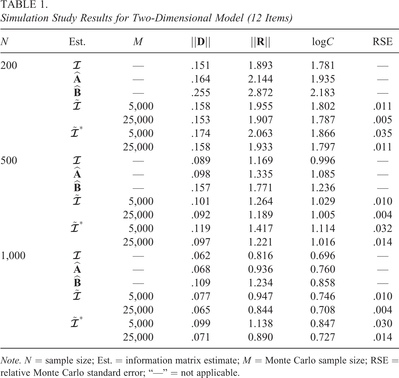
For each IM estimate and sample size, Table 1 presents the means of the outcome measures across the 500 replications. Regarding the accuracy of the estimates, unsurprisingly, the “gold standard” $I$ exhibited the best performance, for all outcome measures and sample sizes. Among the established sample-based estimates, the observed information outperformed the cross-product approximation for all outcomes and sample sizes, which is consistent with previous research (Tian et al., 2012).

Table 1.

Simulation Study Results for Two-Dimensional Model (12 Items)

N	Est.	M	$\| \| D \| \|$	$\| \| R \| \|$	$log C$	RSE
200	$I$	—	.151	1.893	1.781	—
	$\hat{A}$	—	.164	2.144	1.935	—
	$\hat{B}$	—	.255	2.872	2.183	—
	$\tilde{I}$	5,000	.158	1.955	1.802	.011
		25,000	.153	1.907	1.787	.005
	${\tilde{I}}^{*}$	5,000	.174	2.063	1.866	.035
		25,000	.158	1.933	1.797	.011
500	$I$	—	.089	1.169	0.996	—
	$\hat{A}$	—	.098	1.335	1.085	—
	$\hat{B}$	—	.157	1.771	1.236	—
	$\tilde{I}$	5,000	.101	1.264	1.029	.010
		25,000	.092	1.189	1.005	.004
	${\tilde{I}}^{*}$	5,000	.119	1.417	1.114	.032
		25,000	.097	1.221	1.016	.014
1,000	$I$	—	.062	0.816	0.696	—
	$\hat{A}$	—	.068	0.936	0.760	—
	$\hat{B}$	—	.109	1.234	0.858	—
	$\tilde{I}$	5,000	.077	0.947	0.746	.010
		25,000	.065	0.844	0.708	.004
	${\tilde{I}}^{*}$	5,000	.099	1.138	0.847	.030
		25,000	.071	0.890	0.727	.014

Note. N = sample size; Est. = information matrix estimate; M = Monte Carlo sample size; RSE = relative Monte Carlo standard error; “—” = not applicable.

The proposed estimators $\tilde{I}$ and ${\tilde{I}}^{*}$ may also be compared to $I$ , and the differences in the outcomes are attributable to Monte Carlo error. In particular, the differences in results between $\tilde{I}$ and $I$ are due to the Monte Carlo error when simulated response patterns are used instead of the model-implied marginal probabilities. For a fixed value of M, the differences in results between ${\tilde{I}}^{*}$ and $\tilde{I}$ are due to the Monte Carlo error when the unbiased estimate $G^{*} (\hat{γ} | {\tilde{y}}_{i}, {\tilde{θ}}_{i}^{(1)}, {\tilde{θ}}_{i}^{(2)})$ is used instead of the actual individual cross product $G (\hat{γ} | {\tilde{y}}_{i})$ . As expected, for a given M, $\tilde{I}$ was more accurate than ${\tilde{I}}^{*}$ for all sample sizes and outcome measures. However, ${\tilde{I}}^{*}$ with $M = 25, 000$ and $\tilde{I}$ with $M = 5, 000$ yielded similar results. This is notable, as computation for $G (\hat{γ} | {\tilde{y}}_{i})$ used $49^{2} = 2, 401$ integration points, while $G^{*} (\hat{γ} | {\tilde{y}}_{i}, {\tilde{θ}}_{i}^{(1)}, {\tilde{θ}}_{i}^{(2)})$ used just two.

Next, the proposed expected IM estimators were compared to the established observed IM $\hat{A}$ . This comparison is informative because $\hat{A}$ is the most accurate of the established methods that is routinely available. To simplify the comparisons, only the $M = 25, 000$ condition is used. With one exception, both $\tilde{I}$ and ${\tilde{I}}^{*}$ were more precise than $\hat{A}$ . The one exception is that for $N = 1, 000$ and the $| | D | |$ statistic, $\hat{A}$ outperformed ${\tilde{I}}^{*}$ . More generally, the results show that as sample size increases, the proposed estimators and the observed IM perform more similarly.

Regarding the Monte Carlo error for $\tilde{I}$ and ${\tilde{I}}^{*}$ , several aspects of the results are noteworthy. First, the pattern of RSE results is consistent with the results for the measures of accuracy. The lowest RSE values correspond to $\tilde{I}$ with $M = 25, 000$ , the highest values correspond to ${\tilde{I}}^{*}$ with $M = 5, 000$ , and the values for ${\tilde{I}}^{*}$ with $M = 25, 000$ and $\tilde{I}$ with $M = 5, 000$ are comparable. Second, though the RSE results depend on M, they do not appear to depend on N. This is unsurprising, as the RSE statistic quantifies the uncertainty in estimating $I = I (\hat{γ})$ , not $I (γ_{0})$ . Finally, the RSE appears proportional to $M^{- 1 / 2}$ . This is also unsurprising, as it is a basic property of Monte Carlo integration (Robert & Casella, 2013).

4.4.2. Four-dimensional model

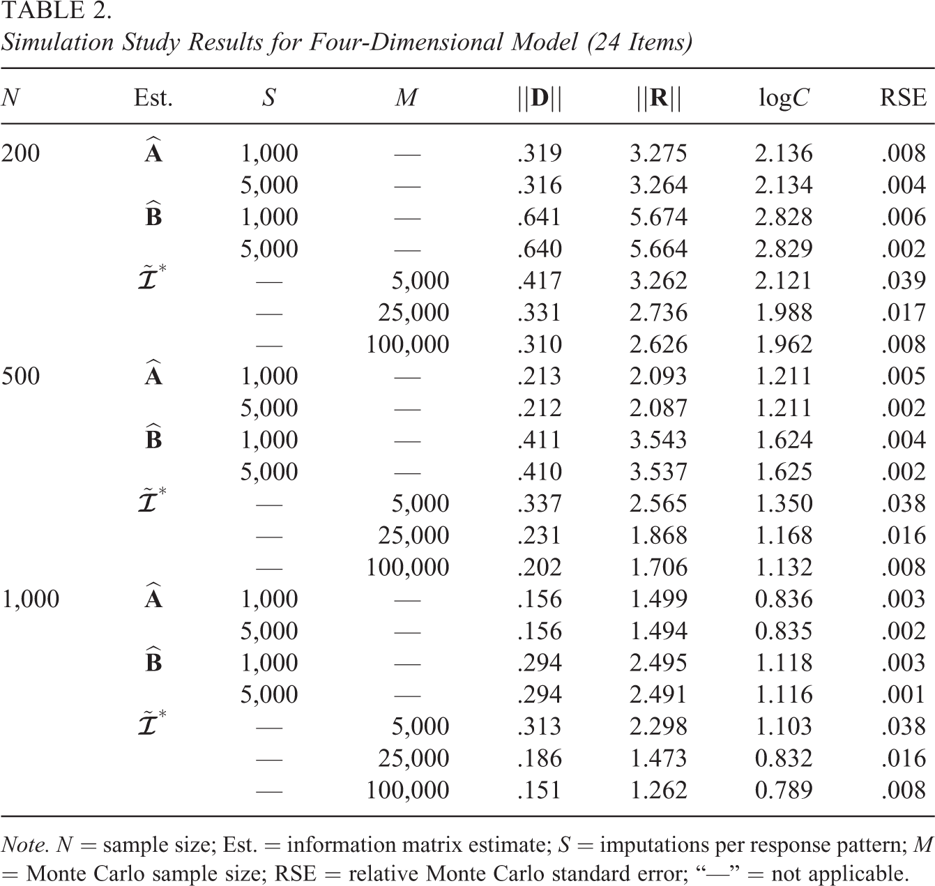
Table 2 presents the means of the outcome measures for $\hat{A}$ , $\hat{B}$ , and the proposed expected IM ${\tilde{I}}^{*}$ . Because $\hat{A}$ and $\hat{B}$ are computed by Monte Carlo for the four-dimensional model, the RSE statistic can be computed for these estimates as well. Just as with the results for the two-dimensional model, Table 2 shows that $\hat{A}$ is more accurate than $\hat{B}$ . For both $\hat{A}$ and $\hat{B}$ , the estimates are more accurate for greater sample sizes N or imputations per response pattern S. However, there is little difference in the accuracy for either $\hat{A}$ or $\hat{B}$ as S is increased from $1, 000$ to $5, 000$ . This suggests there is little Monte Carlo error for the $S = 1, 000$ estimates, which is confirmed by the RSE results. For example, for $\hat{A}$ with $N = 500$ and $S = 1, 000$ , $RSE = 0.005$ , or $0.5 %$ .

Turning to the proposed ${\tilde{I}}^{*}$ , the estimates are more accurate for greater sample sizes N or number of simulated response patterns M. However, the differences in results for the $M = 25, 000$ and $M = 100, 000$ estimates are large enough to suggest there is nonnegligible Monte Carlo error for the $M = 25, 000$ estimates. Again, this may be confirmed by the RSE results, which show $RSE \approx 0.02$ for the $M = 25, 000$ conditions. In contrast, for the $M = 100, 000$ conditions, $RSE < 0.01$ .

Comparing $\hat{A}$ and ${\tilde{I}}^{*}$ , it should first be noted that S and M are not directly comparable. With that said, the RSE results indicate there is less Monte Carlo error for $\hat{A}$ with $S = 5, 000$ than for ${\tilde{I}}^{*}$ with $M = 100, 000$ . Nevertheless, for all sample sizes and outcome measures, ${\tilde{I}}^{*}$ with $M = 100, 000$ is the most accurate estimate. These results are also consistent with the results for the two-dimensional model in Table 1, where, for sufficiently large M, ${\tilde{I}}^{*}$ outperforms $\hat{A}$ . From another perspective, across studied conditions, for sufficiently small RSE (e.g., $RSE \leq 0.01$ ), ${\tilde{I}}^{*}$ outperforms $\hat{A}$ . Thus, for the studied conditions, it is reasonable to conclude that ${\tilde{I}}^{*}$ can provide more accurate estimation than $\hat{A}$ .

5. Empirical Examples

Two empirical data sets were used to compare the proposed IM estimators to the established observed IM, $\hat{A}$ . The first data set is from a Grade 12 science assessment test and is made available in the TESTFACT manual (Wood et al., 2003). The sample size is $N = 572$ , and there are $n = 32$ dichotomously scored items. A unidimensional model was fit to the data, using the 2PL model, yielding 64 total parameter estimates. The observed IM $\hat{A}$ and the expected IM estimate $\tilde{I}$ with $M = 25, 000$ were each computed and used as the basis for a set of standard error estimates. For the $\tilde{I}$ estimate, $RSE = 0.003$ , indicating negligible Monte Carlo error. The two sets of standard error estimates are presented in the left plot of Figure 1. The intercept standard error estimates are, on average, $1 %$ greater for $\hat{A}$ than for $\tilde{I}$ , while the slope standard error estimates are, on average, $3 %$ greater.

Figure 1.

Standard error estimates for empirical examples.

The second data set is from a PISA 2003 (Organization for Economic Cooperation and Development, 2003) student questionnaire surveying mathematical self-belief. A sample of $N = 1, 000$ U.S. students was randomly sampled from the full data set for illustration, and $n = 18$ items, each with four response options, were selected. The items belong to three scales theorized to be interrelated. As such, a three-dimensional simple structure model was fit to the data, using a multidimensional version of the graded response model (Samejima, 1969). This yielded 75 total parameter estimates (54 intercepts, 18 slopes, and 3 latent variable correlations). Following the simulation study, $\hat{A}$ and ${\tilde{I}}^{*}$ were computed, with $S = 5, 000$ and $M = 100, 000$ , respectively. For $\hat{A}$ , $RSE = 0.007$ , and for ${\tilde{I}}^{*}$ , $RSE = 0.015$ . Note that this latter value is slightly larger than the average RSE values reported in Table 2 for $M = 100, 000$ . The two sets of standard error estimates are presented in the right plot of Figure 1. There is no difference, on average, for the intercept standard error estimates for the two IM estimates. In contrast, on average, the slope standard error estimates are $3 %$ greater for $\hat{A}$ than for $\tilde{I}$ , while the correlation standard error estimates are, on average, $6 %$ greater.

Table 2.

Simulation Study Results for Four-Dimensional Model (24 Items)

N	Est.	S	M	$\| \| D \| \|$	$\| \| R \| \|$	$log C$	RSE
200	$\hat{A}$	1,000	—	.319	3.275	2.136	.008
	$\hat{A}$	5,000	—	.316	3.264	2.134	.004
	$\hat{B}$	1,000	—	.641	5.674	2.828	.006
	$\hat{B}$	5,000	—	.640	5.664	2.829	.002
	${\tilde{I}}^{*}$	—	5,000	.417	3.262	2.121	.039
		—	25,000	.331	2.736	1.988	.017
		—	100,000	.310	2.626	1.962	.008
500	$\hat{A}$	1,000	—	.213	2.093	1.211	.005
	$\hat{A}$	5,000	—	.212	2.087	1.211	.002
	$\hat{B}$	1,000	—	.411	3.543	1.624	.004
	$\hat{B}$	5,000	—	.410	3.537	1.625	.002
	${\tilde{I}}^{*}$	—	5,000	.337	2.565	1.350	.038
		—	25,000	.231	1.868	1.168	.016
		—	100,000	.202	1.706	1.132	.008
1,000	$\hat{A}$	1,000	—	.156	1.499	0.836	.003
	$\hat{A}$	5,000	—	.156	1.494	0.835	.002
	$\hat{B}$	1,000	—	.294	2.495	1.118	.003
	$\hat{B}$	5,000	—	.294	2.491	1.116	.001
	${\tilde{I}}^{*}$	—	5,000	.313	2.298	1.103	.038
		—	25,000	.186	1.473	0.832	.016
		—	100,000	.151	1.262	0.789	.008

Note. N = sample size; Est. = information matrix estimate; S = imputations per response pattern; M = Monte Carlo sample size; RSE = relative Monte Carlo standard error; “—” = not applicable.

6. Conclusion

The current research proposed two strategies for estimating the expected Fisher IM. Both strategies use simulated data to calculate a Monte Carlo average and avoid direct integration over all possible response patterns. The first strategy is suitable for low-dimensional models, whereas the second strategy is designed for use with high-dimensional or otherwise complex models. The simulation study demonstrated that both strategies are more accurate than the observed IM, given a sufficiently large Monte Carlo sample size. The empirical examples demonstrated that the proposed methods yield slightly different standard error estimates than those obtained using the observed IM. Notwithstanding these examples, arguably, the newly proposed IM estimators will be most useful in settings where the accuracy of the entire IM estimate is important.

The current work can be extended in several ways. First, the simulation study only considered dichotomous items, but, as demonstrated in the second empirical example, the proposed strategies can be applied to models for polytomous data as well. Future simulation work could focus on such polytomous data models. Second, the method for monitoring the Monte Carlo error deserves further study. The simulation study only considered the RSE statistic based on the norm of the IM estimate, but future research could study alternative statistics. Additionally, it should be possible to automate the determination of the Monte Carlo sample size (Booth & Hobert, 1999). For example, a stopping rule such as $RSE < 0.01$ could be specified. Such a rule would be useful in practice, as the Monte Carlo sample sizes used in the simulation study might not generalize well to applied settings. Third, though the utility of the ${\tilde{I}}^{*}$ estimate was explored using multidimensional IRT models, this estimate can also be applied to other relatively complex IRT models such as multilevel or latent regression IRT models. Finally, the proposed estimators can be applied to other modeling frameworks such as diagnostic classification modeling (Rupp, Templin, & Henson, 2010).

Footnotes

Declaration of Conflicting Interests

The author(s) declared no potential conflicts of interest with respect to the research, authorship, and/or publication of this article.

Funding

The author(s) received no financial support for the research, authorship, and/or publication of this article.

Note

References

Bock

R. D.

Aitkin

(1981). Marginal maximum likelihood estimation of item parameters: Application of an EM algorithm. Psychometrika, 46, 443–459.

Booth

J. G.

Hobert

J. P.

(1999). Maximizing generalized linear mixed model likelihoods with an automated Monte Carlo EM algorithm. Journal of the Royal Statistical Society: Series B, 61, 265–285.

Cai

(2008). SEM of another flavour: Two new applications of the supplemented EM algorithm. British Journal of Mathematical and Statistical Psychology, 61, 309–329.

Cai

(2010). High-dimensional exploratory item factor analysis by a Metropolis–Hastings Robbins–Monro algorithm. Psychometrika, 75, 33–57.

Cai

(2017). flexMIRT® (Version 3.51): Flexible multilevel and multidimensional item response theory analysis and test scoring [Computer software]. Chapel Hill, NC: Vector Psychometric Group.

Chalmers

R. P

. (2018). Numerical approximation of the observed information matrix with Oakes’ identity. British Journal of Mathematical and Statistical Psychology, 71, 415–436.

Diebolt

E. H. S.

(1996). Stochastic EM: Method and application. In Gilks

Richardson

Spiegelhalter

(Eds.), Markov chain Monte Carlo in practice (pp. 259–273). London, England: Chapman and Hall.

Efron

Tibshirani

R. J

. (1994). An introduction to the bootstrap. New York, NY: Chapman and Hall.

Falk

C. F.

Monroe

(2018). On Lagrange multiplier tests in multidimensional item response theory: Information matrices and model misspecification. Educational and Psychological Measurement, 78, 653–678.

10.

Fisher

R. A.

(1925). Theory of statistical estimation. Proceedings of the Cambridge Philosophical Society, 22, 700–725.

11.

Fox

J. P.

(2003). Stochastic EM for estimating the parameters of a multilevel IRT model. British Journal of Mathematical and Statistical Psychology, 56, 65–81.

12.

Gibbons

R. D.

Hedeker

D. R.

(1992). Full-information item bi-factor analysis. Psychometrika, 57, 423–446.

13.

Glas

C. A. W.

(1999). Modification indices for the 2-PL and the nominal response model. Psychometrika, 64, 273–294.

14.

Glas

C. A. W.

Verhelst

(1989). Extensions of the partial credit model. Psychometrika, 54, 635–659.

15.

Liu

Maydeu-Olivares

(2012). Local dependence diagnostics in IRT modeling of binary data. Educational and Psychological Measurement, 73, 254–274.

16.

Lord

F. M.

(1952). A theory of test scores (Monograph No. 7). Chicago, IL: Psychometric Corporation.

17.

Louis

T. A.

(1982). Finding the observed information matrix when using the EM algorithm. Journal of the Royal Statistical Society: Series B, 44, 226–233.

18.

Maydeu-Olivares

(2013). Focus article: Goodness of fit assessment of item response theory models. Measurement: Interdisciplinary Research and Perspectives, 11, 71–101.

19.

Meilijson

(1989). A fast improvement to the EM algorithm on its own terms. Journal of the Royal Statistical Society: Series B (Methodological), 51, 127–138.

20.

Meng

X.-L.

Schilling

(1996). Fitting full-information item factor models and an empirical investigation of bridge sampling. Journal of the American Statistical Association, 91, 1254–1267.

21.

Metropolis

Rosenbluth

A. W.

Rosenbluth

M. N.

Teller

A. H.

Teller

(1953). Equations of state calculations by fast computing machines. Journal of Chemical Physics, 21, 1087–1092.

22.

Monroe

(2018). Contributions to estimation of polychoric correlations. Multivariate Behavioral Research, 53, 247–266.

23.

Oakes

(1999). Direct calculation of the information matrix via the EM. Journal of the Royal Statistical Society: Series B (Statistical Methodology), 61, 479–482.

24.

Organization for Economic Cooperation and Development. (2003). PISA 2003 technical report. Paris: Author.

25.

Paek

Cai

(2014). A comparison of item parameter standard error estimation procedures for unidimensional and multidimensional item response theory modeling. Educational and Psychological Measurement, 74, 58–76.

26.

Pritikin

J. N.

(2017). A comparison of parameter covariance estimation methods for item response models in an expectation-maximization framework. Cogent Psychology, 4, 1279435. doi:10/1080/23311908.2017.1279435

27.

R Core Team. (2016). R: A language and environment for statistical computing [Computer software manual]. Vienna, Austria. Retrieved from https://www.R-project.org/

28.

Ranger

Kuhn

J.-T.

(2012). Assessing fit of item response models using the information matrix test. Journal of Educational Measurement, 49, 247–268.

29.

Robert

Casella

(2013). Monte Carlo statistical methods. New York, NY: Springer Science & Business Media.

30.

Rupp

A. A.

Templin

Henson

R. A.

(2010). Diagnostic measurement: Theory, methods, and applications. New York, NY: Guilford Press.

31.

Samejima

. (1969). Estimation of latent ability using a response pattern of graded scores. Psychometrika Monograph Supplement, 34, 100.

32.

Snijders

T. A. B.

(2001). Asymptotic null distribution of person fit statistics with estimated person parameter. Psychometrika, 66, 331–342.

33.

Spall

J. C.

(2005). Monte Carlo computation of the Fisher information matrix in nonstandard settings. Journal of Computational and Graphical Statistics, 14, 889–909. doi:10.1198/106186005x78800

34.

Tian

Cai

Thissen

Xin

(2012). Numerical differentiation methods for computing error covariance matrices in item response theory modeling: An evaluation and a new proposal. Educational and Psychological Measurement, 73, 412–439.

35.

Tsutakawa

R. K.

(1984). Estimation of two-parameter logistic item response curves. Journal of Educational Statistics, 9, 263–276.

36.

Wei

G. C. G.

Tanner

M. A.

(1990). A Monte Carlo implementation of the EM algorithm and the poor man’s data augmentation algorithm. Journal of the American Statistical Association, 85, 699–704.

37.

White

(1982). Likelihood estimation of misspecified models. Econometrica, 50, 1–25.

38.

Wood

Wilson

Gibbons

R. D.

Schilling

S. G.

Muraki

Bock

R. D.

(2003). TESTFACT 3.0: Test scoring, item statistics, and full-information item factor analysis [Computer software]. Lincolnwood, IL: Scientific Software International.

39.

Yang

J. S.

Hansen

Cai

(2012). Characterizing sources of uncertainty in item response theory scale scores. Educational and Psychological Measurement, 72, 264–290.

40.

Yuan

K.-H.

Cheng

Patton

(2013). Information matrices and standard errors for MLEs of item parameters in IRT. Psychometrika, 79, 232–254. doi:10.1007/S11336-013-9334-4