A Fast and Simple Algorithm for Bayesian Adaptive Testing

Abstract

The Bayesian way of accounting for the effects of error in the ability and item parameters in adaptive testing is through the joint posterior distribution of all parameters. An optimized Markov chain Monte Carlo algorithm for adaptive testing is presented, which samples this distribution in real time to score the examinee’s ability and optimally select the items. Thanks to extremely rapid convergence of the Markov chain and simple posterior calculations, the algorithm is ready for use in real-world adaptive testing with running times fully comparable with algorithms that fix all parameters at point estimates during testing.

Keywords

ability estimation adaptive testing Bayesian optimality Gibbs sampler item calibration item response models MCMC algorithm

Adaptive testing programs typically fix all their parameters at point estimates during testing. Use of point estimates of the item parameters rather than their true values ignores the uncertainty about them when estimating the examinee’s ability. Use of point estimates for the examinee’s parameter as well creates additional uncertainty about the values of the criterion of optimality used to select the items. Ignoring both types of uncertainty leads to the report of standard errors (SEs) for the examinees’ final scores that are generally too optimistic. At the same time, with the current increase in the number of security breaches, high-stakes testing programs feel the need to replenish their item pools more rapidly and consequently are under pressure to reduce the size of their calibration samples, which is only possible at the price of larger error in the item parameters. To accommodate this need, it has even been suggested to introduce new items with subjective initial estimates for their parameters only, updating the estimates using subsequently collected operational data (Makransky & Glas, 2010).

Adaptive testing can be formally characterized as a procedure in which we try to optimize a match between the parameters of the items and the examinee’s ability parameter. When the values of these parameters contain error, the optimization may lead to the selection of items because of the size of these errors rather than the true parameter values. The effects of this capitalization on parameter error were studied first for the problem of optimal selection of fixed test forms by Hambleton and Jones (1994) and Hambleton, Jones, and Rogers (1993) and later for adaptive testing by Cheng, Patton, and Shao (2015), Patton, Cheng, Yuan, and Diao (2013), and van der Linden and Glas (2000, 2001). From these studies, three different factors can be identified to have an impact on the effects. The first factor is the size of the errors in the item parameters in the pool from which the items are selected. Items are typically selected using a criterion of optimality based on their Fisher information at the ability estimate. In this case, the selection process tends to favor items with large positive error in the discrimination parameters, whose squared values appear as a factor in the expression of the information measure for the three-parameter logistic (3PL) model (Equation 5). Second, the number of items selected relative to the size of the pool is an important factor. The smaller the item selection ratio, the greater the likelihood of selecting items with positive estimation error. For adaptive testing, the item selection ratio is actually quite unfavorable; only 1 item at a time is selected, each time from a section of the pool supposed to be optimal at a different ability estimate. The third factor is one that actually mitigates the effects of item parameter error. Real-world adaptive testing programs typically impose constraints on their item selection necessary to guarantee satisfaction of an often large variety of content and statistical specifications and/or to serve more practical goals such as control of the exposure of the items for security purposes. These constraints reduce the effective size of the pool from which the items are selected and, in doing so, create a more favorable item selection ratio.

Hambleton and Jones (1994) selected test items for fixed forms of 10 and 20 items from a pool of 80 items calibrated using the responses of $N = 2,000$ and 500 examinees. These choices of test length and item pool size amount to selection ratios of 8:1 and 4:1, respectively. The authors selected their test forms to have items with maximum values for their estimated discrimination parameters. Plots of the test information functions based on the estimated and true item parameters showed a difference of some 20% in height near the middle of the scale for the unfavorable condition with the smaller calibration sample size and greater selection ratio, whereas the differences were nearly negligible for the reverse combination of the greater sample size and smaller ratio. A replication of the study with a selection ratio of 6:1 and calibration sample sizes of N = 1,000 and 400 examinees showed similar results (Hambleton, Jones, & Rogers, 1993). In their studies of adaptive item selection, van der Linden and Glas (2000, 2001) simulated the use of an item pool with subsets of items calibrated with samples sizes of N = 250, 500, 1,500, and 2,500 items in combination with various test lengths and item selection criteria. For the test length of n = 10, for each of their criteria, the number of items selected during testing from the subset in the pool for N = 250 was generally 5 times larger than for N = 2,500. The difference decreased to a factor of approximately two for a test length of n = 40, while further reduction of the difference was obtained by introducing random item-exposure control as a constraint on the selection of the items. Similar trends were observed by Cheng et al. (2015) and Patton et al. (2013). For their condition with Sympson–Hetter exposure control and a test length of n = 15 items from a pool of 520 items, these authors observed a loss of relative efficiency of the test due to a reduction of the calibration sample size from N = 2,500 to 500 items of some 20% uniformly along the ability scale. The loss should be largely due to the item selection ratio which, for the test length of n = 15 items, was 34:1 in this part of these authors’ study.

The natural framework for dealing with parameter estimation error is a fully Bayesian approach based on the joint posterior distribution of all model parameters. The approach enables us to integrate all item parameters out of the joint distribution to obtain the marginal posterior distribution of the ability parameter to score the examinee. Unlike the SEs traditionally reported in adaptive testing, the standard deviation (SD) of this marginal posterior distribution is for the actual length of the test, avoiding the need to use any asymptotic approximation. Equally important, the approach allows us to adjust the item selection criterion for the uncertainty about all model parameter, just by taking its average across the complete joint posterior distribution.

The first to offer a Bayesian treatment of the problem of ability estimation in the presence of error in the item parameters were Tsutakawa and Johnson (1990) and Tsutakawa and Soltys (1988) who formulated the problem for fixed test forms scored under the 3PL and two-parameter logistic (2PL) models, respectively. Although their formulation was entirely Bayesian, the mathematical complexity of integrating the joint density over all item parameters to score the examinees, for instance, a total of 90 integrals for each examinee on an 30-item test under the 3PL model was simply beyond the computational means of the late 1980s (and still is). The solution they offered was Lindley’s approximation to the posterior mean and variance of the ability parameters with an adjustment for nonnormality. The empirical examples of their approximations already showed substantial improvement over estimation with the item parameters fixed at point estimates. However, though operational use of the approximations is certainly possible for the case of fixed test forms with delayed score reporting, they still are computationally much too intensive for repeated use in real-time adaptive testing. Besides, they only correct the first two moments of the final marginal posterior distribution of the ability parameter but do not give us the complete joint distribution of all parameters required for Bayesian item selection.

With the advent of modern Markov chain Monte Carlo (MCMC) methods (e.g., Gilks, Richardson, & Spiegelhalter, 1996), the challenge of multiple integrals faced by the earlier Bayesian authors has been overcome. Rather than approximating them analytically, these methods generate a Markov chain that simulates draws from the joint posterior distribution of all parameters once it has reached its stationary state, which is continued until the required degree of accuracy for the posterior computations is realized. However, MCMC methods still have the reputation of being slow, certainly for repeated real-time application in operational adaptive testing.

This article presents an MCMC method optimized for use in adaptive testing, which does produce accurate results in extremely short running times. A key feature of Bayesian adaptive testing is sequential updating of the posterior distribution of ability parameter θ of each individual examinee after each new response (as opposed to scoring all examinees afterward as in large-scale fixed-form testing). As the posterior distributions of the parameters of the items in the pool do not change, the update can easily be performed using a Gibbs sampler with a Metropolis–Hastings (MH) step for the posterior distribution of θ, while resampling vectors of draws from the posterior distribution of the parameters of the administered item saved from its calibration. For the 3PL model, the method effectively requires convergence to one unknown posterior distribution of θ in the presence of distributions for 3 item parameters that have already converged. Convergence is boosted further by the use of prior and proposal distributions for the MH step that automatically follow the posterior distribution of the θ parameter during testing. Besides, the criterion for the selection of each next item can be evaluated simply using averages calculated across the sampled values of the ability and item parameters.

The approach is believed to offer at least three advantages over adaptive testing based on point estimates of all parameters. First, as already indicated, it avoids the necessity to report systematically underestimated SEs for the ability estimates typically arrived at through asymptotic approximation, even though adaptive tests are generally much shorter than their fixed-form predecessors. Second, the approach is robust against the impact of capitalization on item parameter error during item selection in adaptive testing. Rather than capitalizing on this error, the approach accounts for it, resulting in an improved design of the test. Third, the approach illustrates a general sequential Bayesian computational scheme that can be used to manage most aspects of automated testing that require real-time parameter updating such as item selection, item calibration, monitoring of item and test security, time management, item-exposure control, and test norming (van der Linden, 2018). The key feature of the scheme is updating the intentional parameters of each of these processes while resampling the current posterior draws for all nuisance parameters. An empirical example already reported elsewhere is real-time item calibration where the focus is on the parameters of field test items added to the pool as intentional parameters and the examinees’ abilities serve as nuisances parameters (van der Linden & Ren, 2015).

The goal of this study was to find optimal settings for the algorithm with respect to such critical factors as the burn-in length of the Markov chain generated by the Gibbs sampler, the required number of post-burn-in iterations for different calibration sample sizes, the size of the item pool, and the length of the test. The study was also conducted to give us estimates of the expected running times of the algorithm when used in real-world testing programs. A final goal of the study was to empirically evaluate the balance between the increase in the SE of the ability parameter estimates and the simultaneous gain due to the improved design of the test relative to current adaptive testing with point estimates and the maximum information (MI) criterion. Ideally, the latter should compensate for the former.

Adaptive Testing

Let $i = 1, . . ., I$ denote the items in the pool and $U_{i} = 0, 1$ the events of a correct and incorrect response to item i for an arbitrary examinee with ability $θ \in ℝ$ . The response model considered is the 3PL model. But, as explained later, the use of the algorithm for any other of the mainstream models in educational and psychological testing requires simple replacement of a few mathematical expressions only.

The 3PL model explains the probability of a correct response as:

$Pr {U_{i} = 1; θ} \equiv p (θ; a_{i}, b_{i}, c_{i}) \equiv c_{i} + (1 - c_{i}) \frac{exp [a_{i} (θ - b_{i})]}{1 + exp [a_{i} (θ - b_{i})]},$
1

where $b_{i} \in ℝ$ and $a_{i} \in ℝ^{^{+}}$ can be interpreted as parameters for the difficulty and discriminating power of item i, respectively, and $c_{i} \in (0, 1]$ as the probability of a correct response to the item resulting from random guessing. The model implies the following probability function for the responses on the items:

$f (u_{i}; θ, ξ_{i}) = p {(θ, ξ_{i})}^{u_{i}} {[1 - p (θ, ξ_{i})]}^{1 - u_{i}},$
2

where $ξ_{i} \equiv (a_{i}, b_{i}, c_{i}) .$

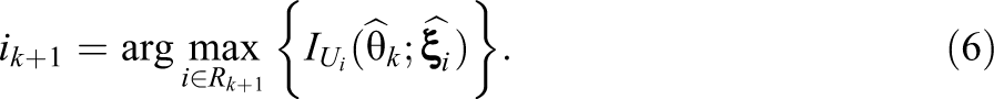
The items in the test are denoted as $k = 1, . . ., n$ , and we use i_k to denote the event of the ith item in the pool selected as the kth item in the test. Suppose k items have already been administered to the examinee, then S_k is the set of indices of these items. The next item in the test has to be selected from $R_{k + 1} = {1, . . ., I} / S_{k}$ .

The common item selection criterion in adaptive testing is the MI criterion, which selects the items to maximize the Fisher information about the ability parameter in the examinee’s responses. For a fixed response to item i, the observed information about θ is measured as

$J_{u_{i}} (θ; ξ_{i}) \equiv - \frac{\partial^{2}}{\partial θ^{2}} ln f (u_{i}; θ, ξ_{i}) .$
3

For a random response, U_i, Fisher’s information is the expected value of Equation 3 across its distribution in Equation 2; that is,

$I_{U_{i}} (θ; ξ_{i}) = E J_{U_{i}} (θ; ξ_{i}),$
4

which for the 3PL model takes the convenient closed form of

$I_{U_{i}} (θ; ξ_{i}) = a_{i}^{2} \frac{1 - p (θ; ξ_{i})}{p (θ; ξ_{i})} {(\frac{p (θ; ξ_{i}) - c_{i}}{1 - c_{i}})}^{2} .$
5

As both the ability and the item parameters are unknown, the typical approach has been to evaluate Equation 5 across all items in $R_{k + 1}$ using point estimates for each of its parameters, selecting the next item as

$i_{k + 1} = arg max_{i \in R_{k + 1}} {I_{U_{i}} (\hat{θ_{k}}; \hat{ξ_{i}})} .$
6

The criterion has been discussed at many places in the literature; for a review of its statistical properties, see van der Linden and Pashley (2010).

In a Bayesian approach, the update of the posterior density of θ upon the examinee’s response to the kth item involves an application of Bayes theorem as

$f (θ | u_{k}) = \frac{\int f (u_{i_{k}} | θ, ξ_{i_{k}}) f (θ | u_{k - 1}) f (ξ_{i_{k}}) d ξ_{i_{k}}}{\int \int f (u_{i_{k}} | θ, ξ_{i_{k}}) f (θ | u_{k - 1}) f (ξ_{i_{k}}) d θ d ξ_{i_{k}}},$
7

where f( $u_{i_{k}}$ | $θ, ξ_{i_{k}}$ ) is the probability of observed response $U_{k i} = u_{k i}$ in Equation 2, f( $ξ_{i_{k}}$ ) is the joint posterior density of the parameters of the item just administered to the examinee, and f( $θ | u_{k - 1}$ ) is the previous posterior density of θ now serving as its prior. Observe that, as all items are assumed to have been calibrated before operational testing, f(θ| $u_{k}$ ) and f( $ξ_{i_{k}}$ ) are independent. The posterior expected version of the criterion of maximum Fisher information in Equation 5 is therefore defined as

$i_{k + 1} = arg max_{i \in R_{k + 1}} {\int \int I_{U_{i}} (θ; ξ_{i}) f (θ | u_{k}) f (ξ_{i}) d θ d ξ_{i}} .$
8

The calculation of Equations 7 and 8 requires integration across the four unknown parameters that drove the examinee’s response to the last item. However, rather than trying to perform the integration, we evaluate it averaging across a sufficiently large sample from the joint distribution of these parameters obtained by the MCMC algorithm in the next section.

MCMC Algorithm

The proposed algorithm is a Gibbs sampler that capitalizes both on the independence of the posterior distributions of θ and $ξ_{i_{k}}$ in Equation 7 and on the sequential nature of adaptive testing. As a result, the sampler iterates extremely efficiently between mutually conditional versions of the two distributions.

More specifically, the proposed implementation of the Gibbs sampler is as follows:

Vectors of draws selected from the last update of the posterior distributions of all parameters have been stored in the system for immediate use.

At each next update of θ, the Gibbs sampler iterates between the following two steps:

Random resampling of the vectors of draws for $ξ_{i}$ for the last item administered to the examinee;

An MH step to sample the distribution of θ.

Once the iterations are concluded, the vector of draws for θ currently stored in the system is overwritten with new draws collected from the stationary part of the Markov chain.

Let $(ξ_{i_{k}}^{(1)}, . . ., ξ_{i_{k}}^{(S)})$ be the vector with the draws $s = 1, . . ., S$ for the parameters of item i_k permanently present in the system and ( $θ^{(1)}, . . ., θ^{(S)}$ ) the most recent update of the vector of draws for the current examinee’s ability parameter θ. The next item is selected calculating the Bayesian criterion of the MI criterion in Equation 8 as

$i_{k + 1} = arg max_{i \in R_{k + 1}} {S^{- 1} \sum_{s = 1}^{S} I_{U_{i}} (θ^{(s)}, ξ_{i}^{(s)})},$
9

that is, simply as the average of the Fisher information in Equation 5 across the available posterior draws of its parameters. The choice of the same length for the vectors of the item and ability parameters is not necessary; for vectors of unequal length, the average should be calculated recycling the shorter vector against the longer. The alternative of averaging overall possible combinations of $ξ_{i}^{(s)}$ and $θ^{(s)}$ is computationally excessive, would involve repeated use of the same draws, and does therefore not add any extra information.

MH Step

Recall that, under mild conditions always met for operational adaptive testing under the 3PL model, the posterior distribution of θ converges to a normal distribution centered at its true value (Chang & Ying, 2009). An obvious choice of prior and proposal distribution during each MH step is therefore a normal with moments derived from the previous posterior update of θ. Let ( $θ_{k - 1}^{(1)}, . . ., θ_{k - 1}^{(S)}$ ) denote the vector of draws stored from this update and $r = 1, 2, . . ., R$ , the new iterations of the sampler (generally, $S < R$ because of post-burn-in thinning of the chain; see below). More specifically, using

$μ_{k - 1} \equiv S^{- 1} \sum_{s = 1}^{S} θ_{k - 1}^{(s)}$
10

and

$σ_{k - 1}^{2} \equiv S^{- 1} \sum_{s = 1}^{S} {(θ_{k - 1}^{(s)} - μ_{k - 1})}^{2},$
11

the choice of prior density of θ during its update after the kth item is

$f_{k - 1} (θ) \equiv N (μ_{k - 1}, σ_{k - 1}^{2}),$
12

while as proposal density we use

$q_{k} (θ | θ_{k}^{(r - 1)}) \equiv N (θ_{k}^{(r - 1)}, σ_{k - 1}^{2}) .$
13

Given the symmetry of Equation 13, the MH step for the rth draw during this update of the posterior distribution of θ simplifies to

draw candidate value $θ^{(c)}$ for $θ_{k}^{(r)}$ from the proposal density $q_{k} (θ | θ_{k}^{(r - 1})$ in Equation 13;

accept $θ_{k}^{(r)} = θ^{(c)}$ with probability
$min {\frac{f_{k - 1} (θ^{(c)}) f (u_{i_{k}}; θ^{(c)}, ξ_{i_{k}}^{(r)})}{f_{k - 1} (θ_{k}^{(r - 1)}) f (u_{i_{k}}; θ_{k}^{(r - 1)}, ξ_{i_{k}}^{(r - 1)})},1};$
14

otherwise keep the draw from the previous iterative step, $θ_{k}^{(r - 1)}$ .

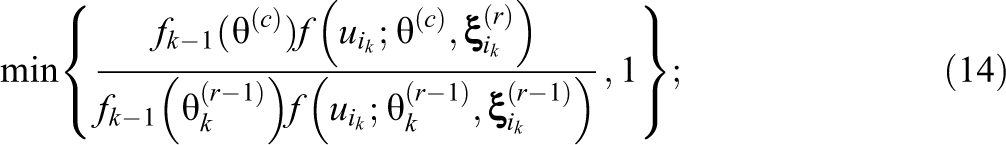
In most applications of Gibbs samplers with MH steps, tuning of the proposal distribution to create acceptance rates in the optimal range of 30%–40% is a time-consuming task. If its scale parameter is chosen to be too great, the number of rejected draws becomes too large. For scale parameters that are too small, the chain converges more slowly than necessary. The proposal distribution in Equation 13 does not require any tuning though. Its location automatically follows that of the current posterior distribution with a variance that is always somewhat greater, which has been proven to be an efficient choice for samplers for low-dimensional parameters (Gelman et al., 2014, section 12.2).

Computationally, everything is extremely simple. The only quantities that need to be calculated are (1) the averages in Equations 10 and 11 and (2) the product of the prior density and the probability of the kth response in the numerator of the acceptance probability in Equation 14 (its denominator was the numerator in the preceding iteration step and need not be recalculated). Unlike adaptive testing with maximum-likelihood estimation of θ, there is no product likelihood with a number of factors that grow during the test; instead, the entire history of each examinee is captured in the most recent posterior distribution of his or her ability parameter. For the selection of the next item, the only necessary quantity to compute is the simple average in Equation 9.

Observe that Equation 12 involves a normal approximation of the prior distribution of θ only. Although the approximation may seem to be reminiscent of Owen’s (1969, 1975) first attempt at a Bayesian approach to adaptive testing, it differs fundamentally in that Owen’s approach was based on item selection with a normal approximation of the posterior distribution, whereas in our approach, the actual posterior distribution is just sampled (including the final posterior distribution used to report the examinee’s ability estimate). Also, only the shape of the prior distribution is taken to be normal; its mean and variance are still empirical. The impact of the choice of a prior on its posterior distribution is generally known to consist of bias toward the mean of the prior with a size dependent on its variance. However, in adaptive testing, ability estimates invariably are close to the true value after some 5 to 7 items (the rest of the test is basically to reduce the size of the SE to an acceptable level). At this point, possible bias toward the empirical prior mean is already negligible. The larger variance of the prior distribution during the first few items in the test is most welcome; it avoids unwarranted stability of the initial bias. If for some reason a normal shape for the prior distribution of the ability parameter would be undesirable, an alternative is to use smooth estimates of the previous posterior density at $θ^{(c)}$ and $θ_{k}^{(r - 1)}$ in Equation 14, for instance, kernel estimates (for details, see van der Linden & Ren, 2015). However, the authors have not found the option to be worth its additional computational complexity.

The assumption of a normal proposal distribution in Equation 13 is pretty much standard practice in the world of MH within Gibbs sampling. It does have an impact on the speed of convergence of the algorithm but not on the statistical properties of the converged results. The main concern of choosing a proposal density is adequate coverage of the intended posterior distribution. As just argued, the fact that our choice of prior automatically follows the posterior distributions with a scale somewhat greater than the latter does guarantee this.

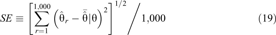
Monte Carlo Error

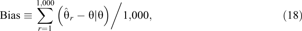
Posterior results obtained from Gibbs samplers have Monte Carlo error. However, the error can be reduced to negligible size just by continuing the iterations after burn-in. In order to calculate the required number of these iterations, the following argument can be applied: Our interest is in reporting the posterior mean of the θ parameter to the examinee. After n items, the mean is estimated with uncertainty equal to the posterior variance $σ_{n}^{2}$ . The Monte Carlo error added to the uncertainty by sampling the posterior distribution is equal to $σ_{n}^{2} / S$ , where S is the effective sample size produced by the Markov chain. Hence, the total error after n item is equal to

$\sqrt{σ_{n}^{2} + σ_{n}^{2} / S} = σ_{n} \sqrt{1 + 1 / S .}$
15

The equation shows that even for small sample sizes, the impact of the Monte Carlo error already becomes negligible. For instance, for $S = 100$ , 250, and 500, the increase in the SE due to the factor $\sqrt{1 + 1 / S}$ in Equation 15 is already as small as 0.49%, 0.25%, and 0.10%, respectively. The effective sample size is known to be equal to

$S = \frac{R}{\sqrt{1 + 2 \sum_{l = 1}^{\infty} ρ_{l}}},$
16

where R now is the total number of post-burn-in iterations of the Markov chain and $ρ_{l}$ is their autocorrelation at time lag l (Gelman et al., 2014, section 11.5).

In the interest of efficient memory management, an obvious strategy is to find the lag size $l^{}$ at which $ρ_{l}$ becomes negligible and use the knowledge to thin the post-burn-in part of the chain to yield a sample of S independent draws. The required total number of post-burn-in iterations is then equal to R = $l^{} S .$ If memory management is less of a concern, we could just limit the sum in the denominator of Equation 16 at $l^{}$ , calculating the required number of iterations as

$R = S \sqrt{1 + 2 \sum_{l = 1}^{l^{}} ρ_{l}},$
17

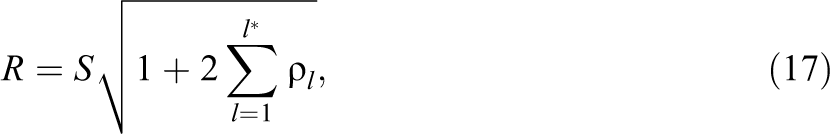
and save all iterations.

Empirical Studies

Several simulation studies were conducted to (1) optimize the Gibbs sampler for use in adaptive testing under a variety of possible conditions and (2) evaluate the impact of the proposed Bayesian approach on the statistical properties of the final ability estimates. Specifically, the first set of studies was to find the minimal choice for the burn-in length of the Markov chain and the required number of post-burn-in iterations under various conditions. They were also conducted to give us estimates of the running times of the algorithm required for these choices. The second set of studies was to evaluate the approach using such statistical quantities as the SE and bias functions of the final θ estimates. As already indicated, one consequence of ignoring all parameter uncertainty in current MI adaptive testing is systematic underestimation of the error in these estimates. Another is less than optimal design of the test. The second set was conducted to assess to what extent improved Bayesian design of the test would compensate for a more realistic estimate of the SE.

General Setup

A pool of 210 items was randomly sampled from an inventory of previously used operational items that had been shown to fit the 3PL model in Equation 1. Figure 1 shows the empirical distributions of the values of the item parameters. The ranges were [0.41, 2.08], [−2.44, 2.96], and [0.10, 0.32] for the a_i, b_i, and c_i parameters, respectively, with means (SDs) equal to 1.08 (0.35), 0.16 (1.22), and 0.21 (0.03). All simulations were for adaptive tests with a length of n = 10, 20, and 30 items. 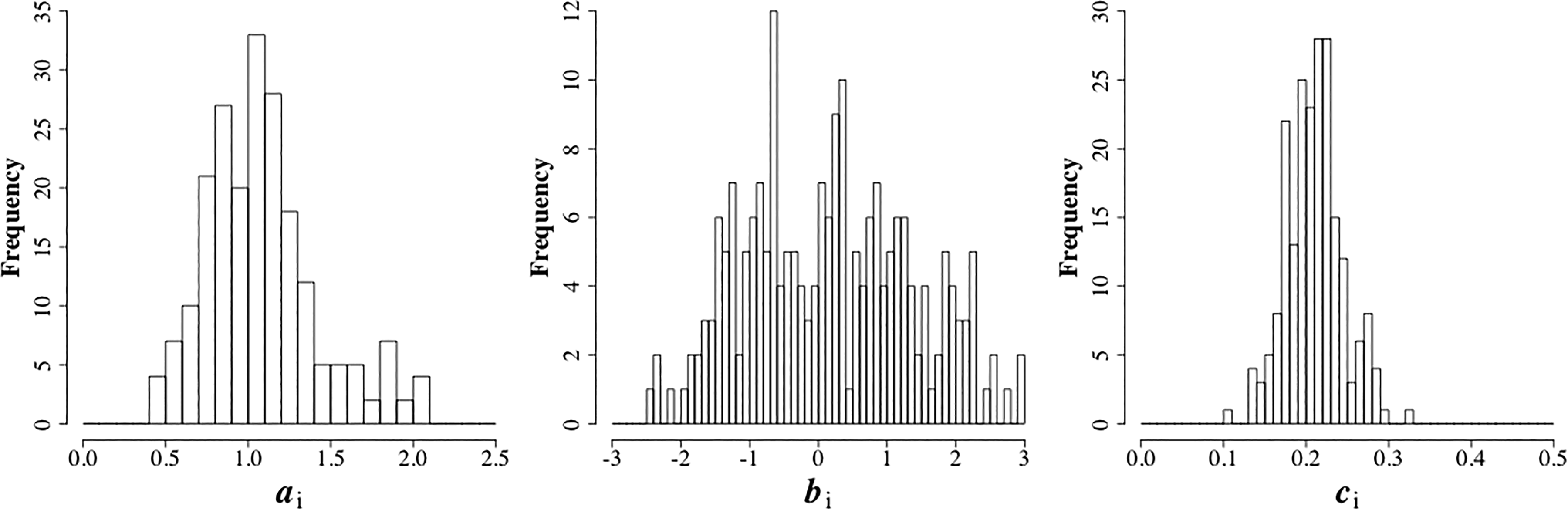The size of the item pool was chosen to be just over 10 times the middle test length of $n = 20$ items. An item pool 7 times the length of the longest tests is somewhat on the smaller side. But we had to compromise to keep the results for all three test lengths comparable and a factor of seven is not too far out of the range of what is usual in the adaptive testing literature (e.g., Stocking, 1994). The simulations were run in R on a MacBook Pro with an Intel Core i7 CPU, 2.5 GHz, and 16 GB of RAM, with the computationally more intensive procedures programmed in Rcpp.

Figure 1.
Empirical distributions of parameters a_i, b_i, and c_i in the item pool.

Three different sets of calibration data of size $N = 250, 500$ , and 1,000 were generated from the item parameters for examinees with ability parameters sampled from a standard normal distribution. The different samples sizes were chosen to evaluate the impact of item calibration error on the various results from our simulations. The first two sizes were intentionally chosen to be small relative to what is usual for item calibration in the testing industry, where a minimum of 1,000 examinees seems to be more of a standard. The responses were generated for a linked calibration design with the items randomly assigned to 21 subsets of 10 items. Each form consisted of two of these subsets, with one common set between Forms 1 and 2, Forms 2 and 3, and so on. The items were calibrated using a regular MH within Gibbs procedure as implemented in JAGS (Plummer, 2017) with a burn-in of 5,000 iterations and continued sampling from the stationary chain for 15,000 iterations. The prior distributions used in the calibration were $θ \sim N (0, 1)$ , $a_{i} \sim N (1,0 {.5}^{2}) I (a_{i} > 0)$ , $b_{i} \sim N {(0, 2}^{2})$ , and $c_{i} \sim Beta (2,5)$ . Use of the procedure was deemed necessary because of the smallest two calibration sample sizes in this study. For existing item banks calibrated with large samples, a practical alternative is to just draw random values for the parameters from normal distributions with means and SDs based on their MML estimates and SEs.

Figure 2 shows plots of the posterior means of the 3-item parameters versus their true values. Clearly, the best results were obtained for the sample size of N = 1,000. The recovery of the b_i parameters was relatively best among the three kinds of parameters, with good results even for the two lower sample sizes. The plots for the critical a_i parameters show considerable scatter for each of the three sample sizes, obviously with larger scatter for the smaller sizes. For the largest sample size, most of the scatter was observed at the upper end of the scale. For the c_i parameters, the choice of sample size did not have much of an impact. A summary of these results is given in Table 1.

Figure 2.
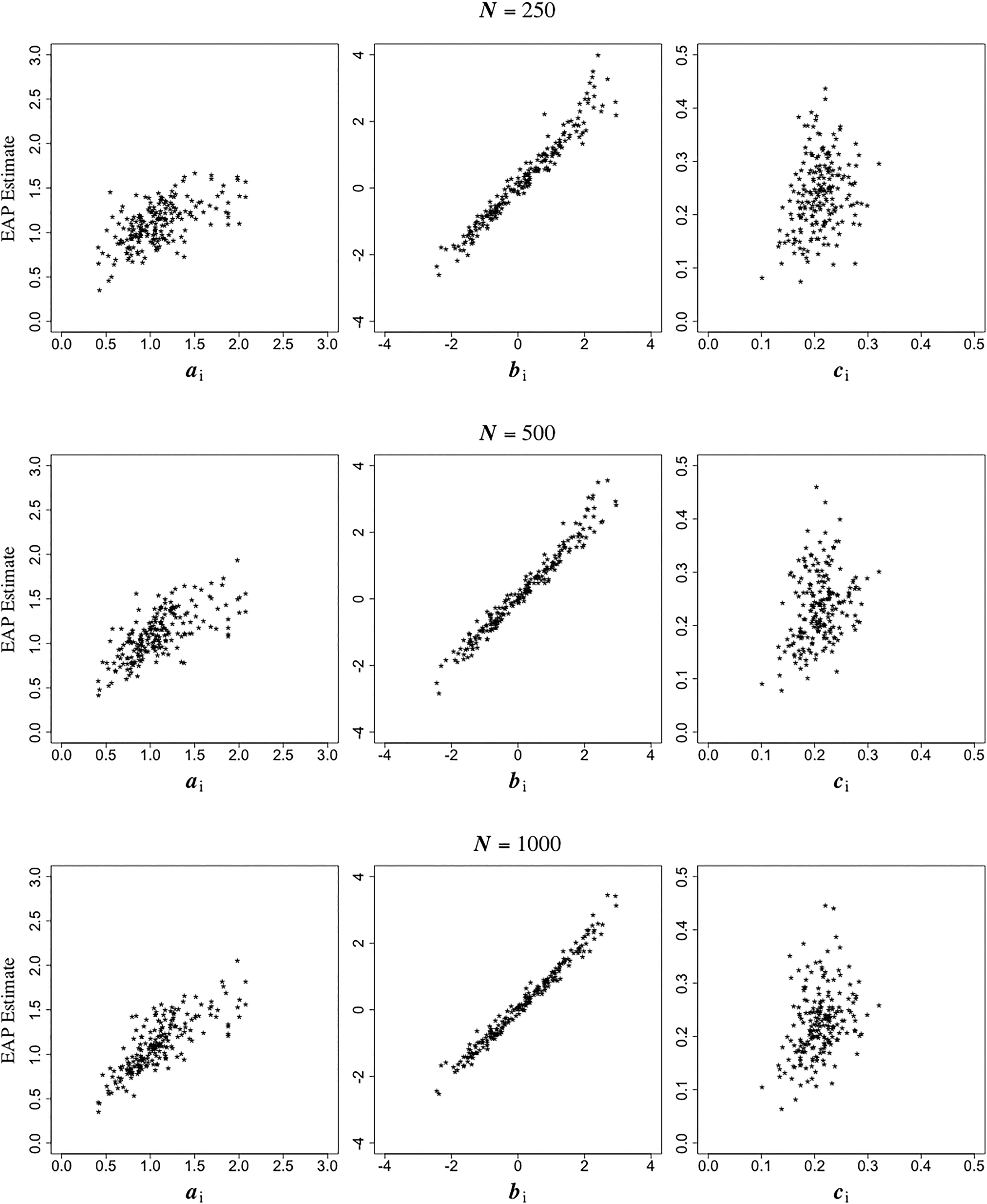
EAP estimates versus true item parameter values after item calibration with sample sizes of N = 250, 500 and 1,000.

Table 1.
Mean, SD, and RMSE of Item Pool Parameter Estimates

Mean SD RMSE

Sample Size a_i b_i c_i a_i b_i c_i a_i b_i c_i

250 .105 .097 .029 .276 .305 .067 .276 .319 .073

500 .018 .090 .025 .247 .243 .063 .247 .258 .068

1,000 .025 .048 .015 .206 .177 .059 .207 .183 .061

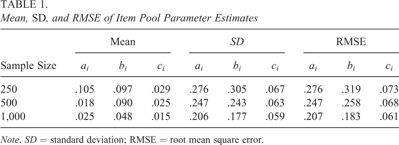
Note. SD = standard deviation; RMSE = root mean square error.

The criterion of effective sample size in Equation 16 was used to determine the length of the vectors of draws from the posterior distributions of the item parameters in the pool to be saved for use in adaptive testing. Figure 3 shows the autocorrelation plots for the posterior draws for the item parameters for each of the three calibration samples produced during the stationary part of the Markov chain as a function of the lag size, l. For a choice of $ρ_{l}$ not larger than 0.10, a critical size of $l^{*}$ = 30 appears to suffice for all three sample sizes. The post-burn-in part of the chain was therefore thinned taking every 30th iteration creating a sample of S = 500 draws for each of the item parameters to be stored in the system for use during adaptive testing. This choice of an effective sample size of 500 is quite conservative; as already noted, it amounts to the acceptance of a Monte Carlo error of 0.10 % of the posterior SD. (As an aside, observe the tendency of the autocorrelation to increase with the calibration sample size for a given lag. The finding seems to point at a stronger autocorrelation for a narrower posterior distribution for the item parameters under the 3PL model. Although authors did notice the effect, they admit to be unable to offer a satisfactory explanation for it.)

Figure 3.
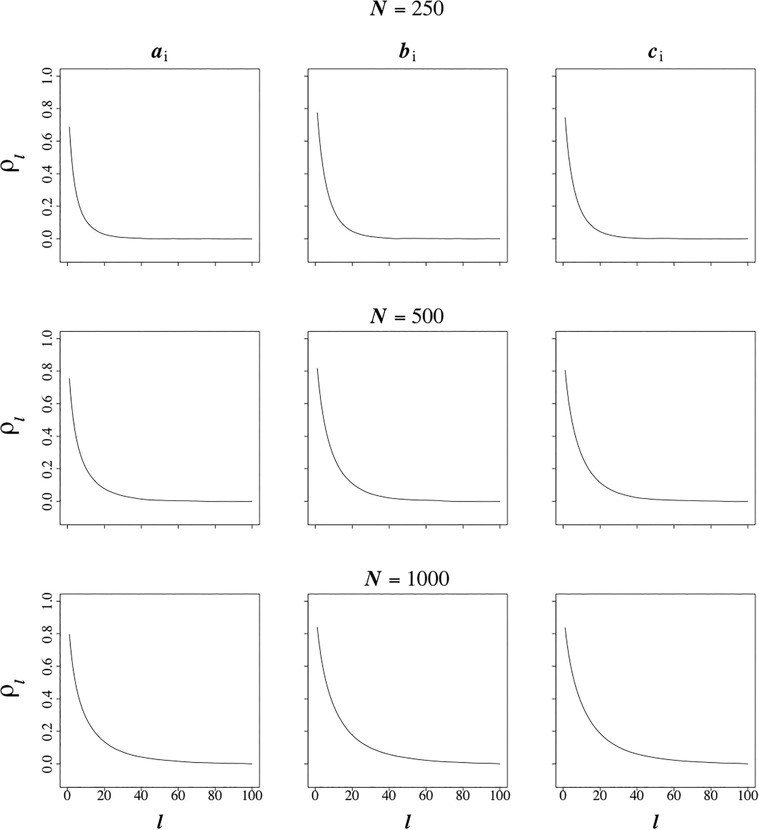
Autocorrelation ρ_l in the Markov chains for the items parameters as a function of lag size l for each of the calibration sample sizes of N = 250, 500, and 1,000.

Pre- and Post-Burn-In

The goal of the main part of our study was to find the necessary length for burn-in of the Markov chain for θ during adaptive testing, the required number of additional iterations, and the best size for the vectors of the draws for θ to be saved for the calculation of the item selection criterion in Equation 9. Adaptive tests were simulated using the Bayesian algorithm exactly as introduced above with vectors of draws for the item parameters set at the level of S = 500 used throughout our simulations. All responses were generated for simulated examinees with true ability parameter values of $θ = - 2 (1) 2$ and the true values of the item parameters in the pool. The initial prior distribution of θ always was $N {(0, 1.5}^{2})$ .

Our first step was to visually inspect several trace plots for the speed of convergence. Figure 4 shows a few typical examples of the first 2,000 draws of the chain for simulated examinees recorded after k = 1(5)26 items. 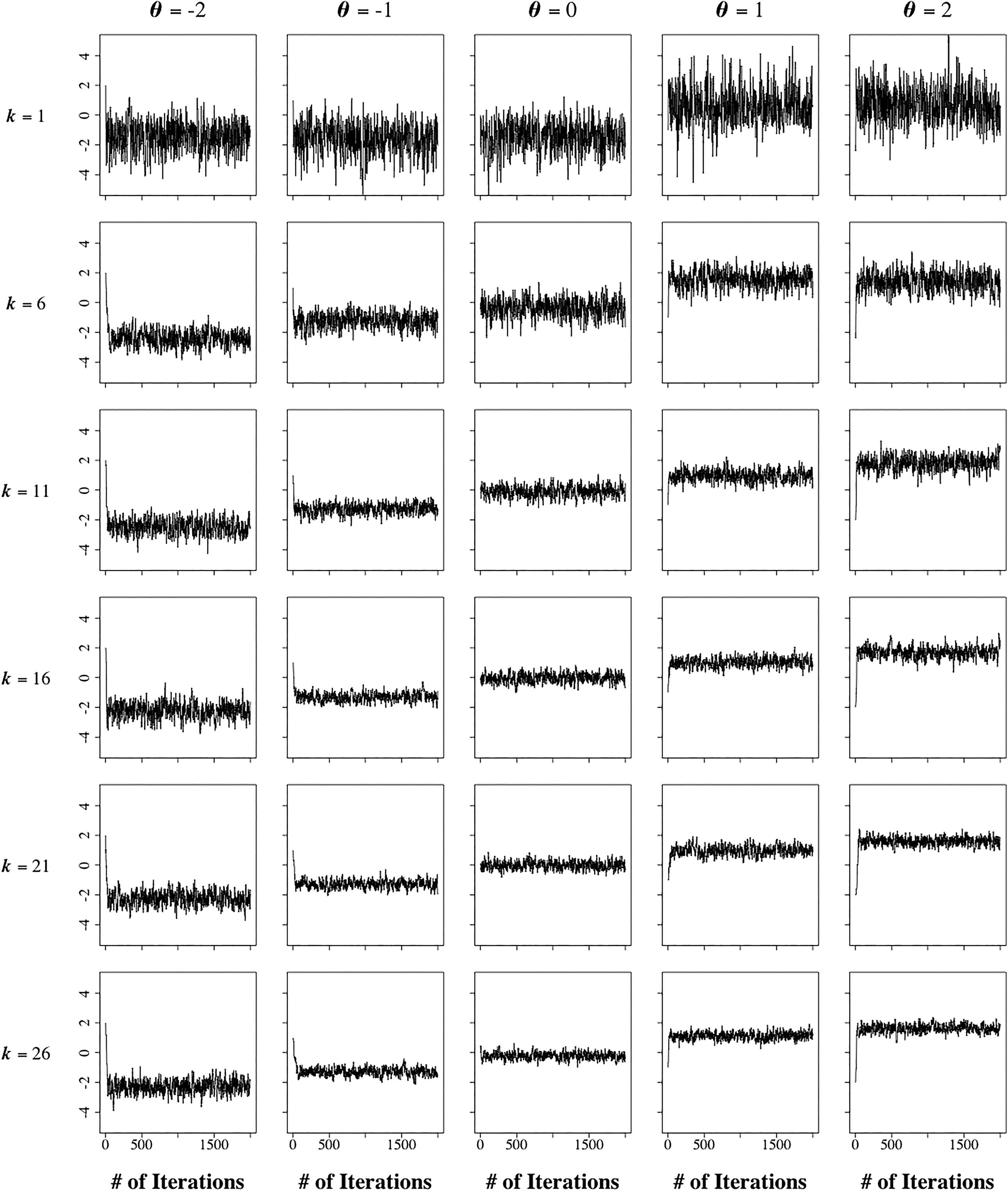To be able to present robust results, the chains were initialized choosing starting values with signs opposite to the true value of the ability parameter; for instance, a starting value of $θ = + 2$ for an examinee at $θ = - 2$ . Each of the plots shows immediate convergence, even after 1 item and examinees with the more extreme true values of $θ = - 2$ and 2. When the number of item administered increases, the chains tend to concentrate at the true θ values with decreasing variances, a trend already clear after k = 6 items.

Figure 4.
Examples of the first 2,000 iterations of the Markov chain Monte Carlo algorithm during the posterior updates of the ability parameter after k = 1(5)26 items for examinees simulated at θ = −2(1)2.

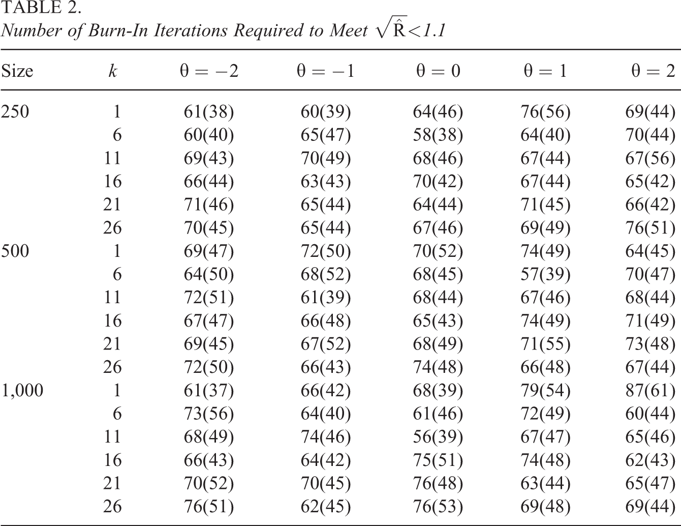
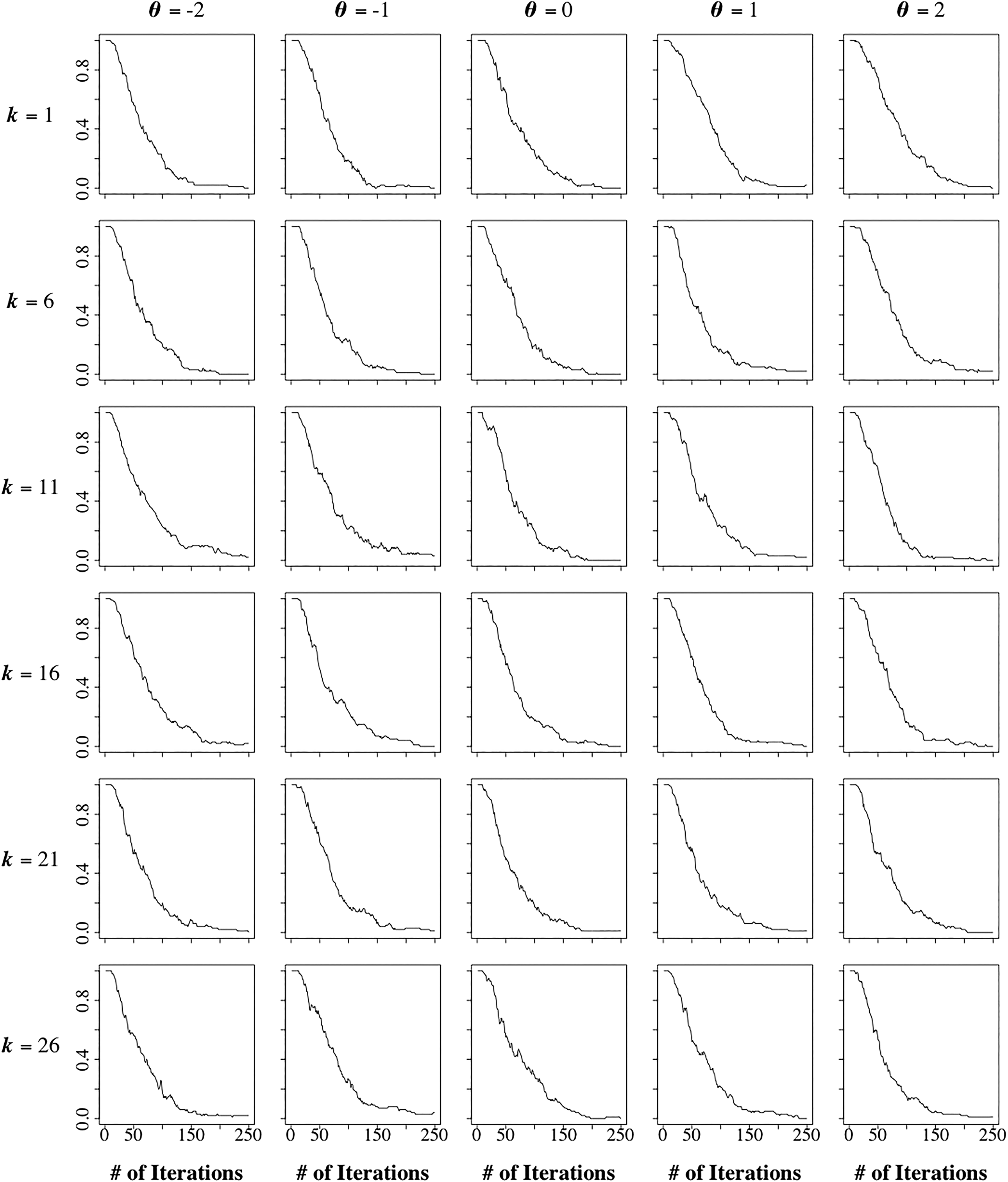
The minimum length of burn-in was determined using the well-known Gelman and Rubin (1992) statistic for multiple MCMC chains, $\sqrt{\hat{R}}$ . During each replication, four parallel chains were started. To obtain the necessary overdispersion of the starting values for the diagnostic to work, the values for two of the chains were randomly sampled from the lower tail of the initial prior distribution of the ability parameters ( $θ < mean - 2 S D$ ) and the other two from its upper tail ( $θ > mean + 2 S D)$ . The four chains were supposed to be mixed when $\sqrt{\hat{R}} < 1.1$ , a usual choice in the literature. For each true value of $θ = - 2 (1) 2,$ the simulation was replicated 100 times.

Table 2 shows the averages and SDs of the number of iterations required to meet the criterion as a function of k = 1(6)26 for each of the five simulated θ values and three calibration sample sizes. None of these factors did appear to have any systematic impact on the number of iterations required for the chains to mix. Figures 5 and 6 show plots with the proportions of replications failing to meet the criterion of $\sqrt{\hat{R}} < 1.1$ as a function of the number of iterations for the calibration sample sizes of N = 250 and 1,000 (the plots for N = 500 were indistinguishable from those for the other two sizes and are omitted to avoid redundancy). Basically, the curves in these plots were identical across all conditions. As none of their replications required more than 250 iterations to meet the criterion, the length of the burn-in in all subsequent simulations was set at these 250 iterations.

Table 2.
Number of Burn-In Iterations Required to Meet $\sqrt{\hat{R}} < 1.1$

Size k $θ = - 2$ $θ = - 1$ $θ = 0$ $θ = 1$ $θ = 2$

250 1 61(38) 60(39) 64(46) 76(56) 69(44)

6 60(40) 65(47) 58(38) 64(40) 70(44)

11 69(43) 70(49) 68(46) 67(44) 67(56)

16 66(44) 63(43) 70(42) 67(44) 65(42)

21 71(46) 65(44) 64(44) 71(45) 66(42)

26 70(45) 65(44) 67(46) 69(49) 76(51)

500 1 69(47) 72(50) 70(52) 74(49) 64(45)

6 64(50) 68(52) 68(45) 57(39) 70(47)

11 72(51) 61(39) 68(44) 67(46) 68(44)

16 67(47) 66(48) 65(43) 74(49) 71(49)

21 69(45) 67(52) 68(49) 71(55) 73(48)

26 72(50) 66(43) 74(48) 66(48) 67(44)

1,000 1 61(37) 66(42) 68(39) 79(54) 87(61)

6 73(56) 64(40) 61(46) 72(49) 60(44)

11 68(49) 74(46) 56(39) 67(47) 65(46)

16 66(43) 64(42) 75(51) 74(48) 62(43)

21 70(52) 70(45) 76(48) 63(44) 65(47)

26 76(51) 62(45) 76(53) 69(48) 69(44)

Figure 5.
Proportion of replications failing to meet the convergence criterion of $\sqrt{\hat{R}} < 1.1$ as a function of the number of iterations after k = 1(5)26 items for examinees simulated at θ = −2(1)2 and a calibration sample size of N = 250.

Figure 6.
Proportion of replications failing to meet the convergence criterion of $\sqrt{\hat{R}} < 1.1$ as a function of the number of iterations after k = 1(5)26 items for examinees simulated at θ = −2(1)2 and a calibration sample size of N = 1,000.

The final decision on the use of the algorithm was with respect to the number of post-burn-in iterations necessary for item selection in adaptive testing. To estimate the autocorrelation of the chain as a function of the time lag, adaptive tests were simulated with 100 replications at each of the true values of $θ = - 2 (1) 2$ . Each of the chains was thus run with 250 iterations for burn-in. It was then continued for an extra of 15,000 iterations to investigate its autocorrelation. The plots in Figures 7 and 8 show the average autocorrelation functions across replications for the calibration sample sizes of N = 250 and 1,000 (again, the plots for N = 500 were indistinguishable from those for the other two sizes). Each of the plots reveals a virtually identical shape of the functions, no matter the true θ value, the number of items already administered, and the size of calibration error. For a choice of $ρ_{l}$ not larger than 0.1, the value of l = 10 emerges as a nearly universal result. It was therefore decided to thin the post-burn-in part of the future chains by taking every 10th iteration.

Figure 7.
Autocorrelation ρ _l in the Markov chains for the ability parameter as a function of lag size l after k = 1(5)2 items for examinees simulated at θ = −2(1)2 and a calibration sample size of N = 250 (solid curves: mean; dashed curves: 5th and 95th percentiles).

Figure 8.
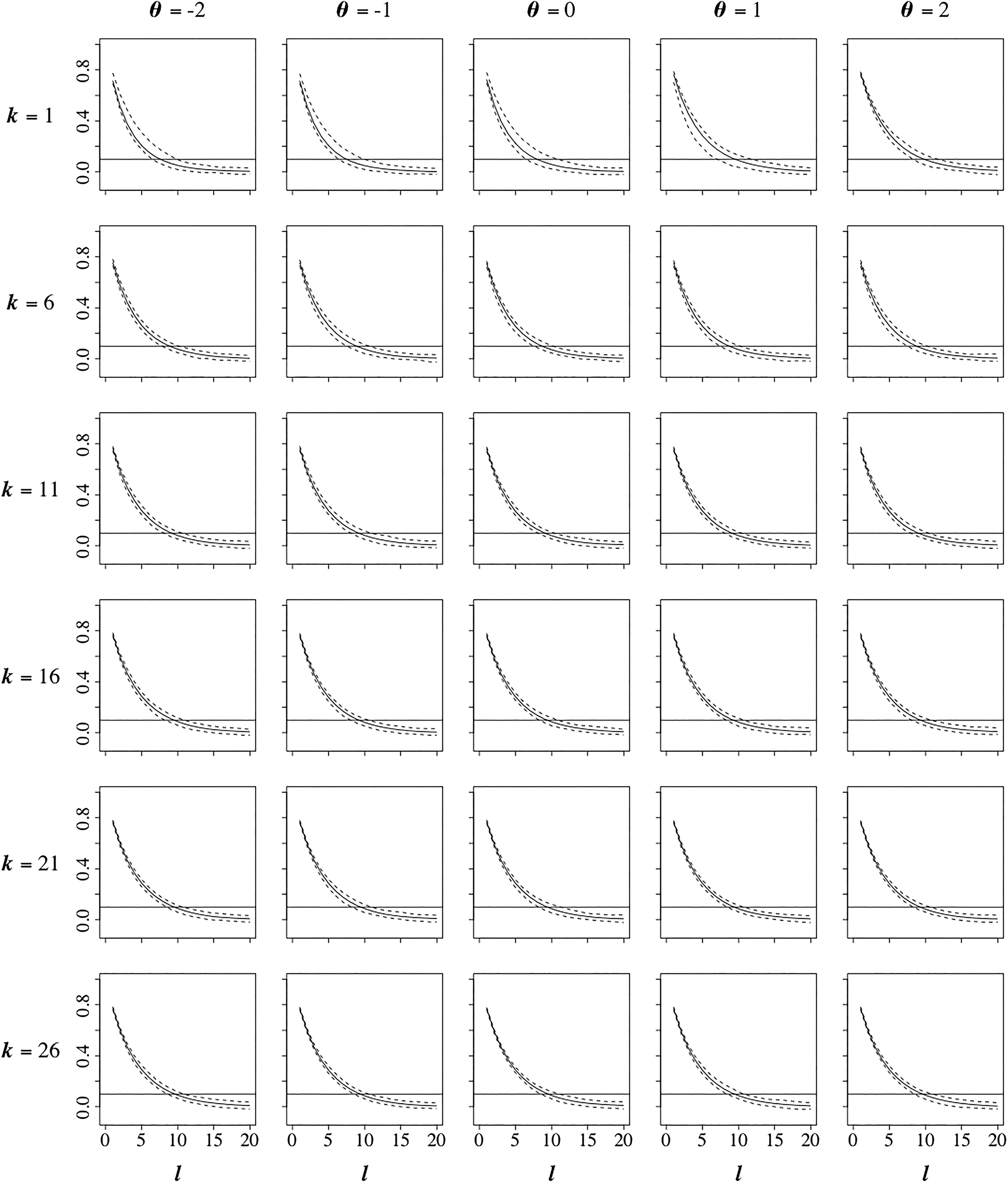
Autocorrelation ρ_l in the Markov chains for the ability parameter as a function of lag size l after k = 1(5)26 items for examinees simulated at θ = −2(1)2 and a calibration sample size of N = 1,000 (solid curves: mean; dashed curves: 5th and 95th percentiles).

In order to determine the size of the vector of draws of θ to be saved from the thinned chain, adaptive tests of n = 30 items were simulated saving vectors of length of S = 100, 200, and 500 draws from the posterior distribution of θ (implying the necessity of 1,000, 2,000, and 5,000 post-burn-in iterations given the chosen thinning factor, respectively). Figure 9 shows the estimated bias and SE functions calculated from 100 replications at $θ = - 2 (1) 2$ each. The bias functions were nearly identical across all three calibration samples sizes, but the SE functions did show improvement for the larger values of S. Apparently, in spite of the seemingly negligible differences in Monte Carlo error between the three choices (0.49%, 0.25%, and 0.01%, respectively), these differences did appear to have an impact on the design of the test, most likely on the choice of the first items when the posterior distribution of θ is still relatively wide.

Figure 9.
Bias and standard error of the final ability estimates after n = 30 items for examinees simulated at θ = −2(1)2, vectors of S = 100 (dotted curves), 200 (dashed curves), and 500 draws (solid curves) saved after each posterior update, and calibration sample sizes of N = 250, 500, and 1,000.

Running Times

The average running time across all replications during the simulations with the vector lengths of S = 100, 200, and 500 for the saved draws for θ was 0.009, 0.012, and 0.015 seconds per item, respectively. Based on all these results, it was decided to run all remaining simulations for S = 500 draws for θ from the thinned stationary part of the chain during the test.

Adaptive Testing Results

Our final simulations were to evaluate the performance of the proposed Bayesian algorithm for the choices of 250 burn-in and 500 × 10 = 5,000 post-burn-in iterations, each time saving $S = 500$ independent post-burn-in draws for the posterior calculations. The simulated test lengths were n = 10, 20, and 30 items. The final ability estimates for the Bayesian and MI algorithm were compared averaging the results from 1,000 examinees simulated at each true ability value θ = −2(1)2. The estimates for the Bayesian algorithm were just the average draws from the final posterior updates, while the expected a posteriori (EAP) estimates for the MI algorithm were calculated using grid approximation over −8(.1)8. The same approximation was used during the test to calculate the point estimates of θ for the selection of the next item by the latter. The comparisons between the two different estimates were made calculating their bias, SE, and root mean square error (RMSE) functions as

$Bias \equiv \sum_{r = 1}^{1,000} ({\hat{θ}}_{r} - θ | θ) / 1,000,$
18

$S E \equiv {[\sum_{r = 1}^{1,000} {({\hat{θ}}_{r} - \bar{\hat{θ}} | θ)}^{2}]}^{1 / 2} / 1,000$
19

and

$RMSE \equiv {[\sum_{r = 1}^{1,000} {({\hat{θ}}_{r} - θ | θ)}^{2}]}^{1 / 2} / 1,000,$
20

respectively, where $\bar{\hat{θ}}$ was the average estimate over each of the 1,000 replications. For both algorithms, the same initial prior distribution of $θ \sim N (0,1.5)$ was used.

Figures 10 through 12 report each of these three functions for the calibration samples of N = 250, 500, and 1,000 examinees. The differences between the two algorithms follow the same pattern for all three sample sizes; however, the smaller the size, the more pronounced the pattern. Interestingly, the bias functions for the two algorithms showed an opposite trend with an increase of test length. The Bayesian algorithm began with an inward bias, but as more responses were collected, the bias disappeared and the functions approximated their desired flat shape. Apparently, the prior distribution served as an effective initial buffer against a data-driven outward bias for this algorithm, which became less necessary when more responses were collected. On the other hand, the MI algorithm began with a flat function for n = 10 but produced functions with an outward bias for n = 20 and 30. The SE functions for the Bayesian algorithm ran practically flat across all conditions, but at a lower height for a larger test length, of course. The same was the case for the MI algorithm for $θ \geq 1$ . However, at the lower end of the scale, this algorithm showed a substantially greater SE across all simulated conditions, precisely the end where greater estimation error occurs due to the guessing assumed by the 3PL model. The Bayesian algorithm acknowledged the error during item selection and produced ability estimates with SEs similar to those across the rest of the scale. The MI algorithm ignored it and paid a price in the form of larger SEs. Generally, plots with RMSE functions are an excellent way to visualize how differences in bias and SE may compensate each other. All plots show negligible differences between these functions for the two algorithms, except at $θ < - 1$ where more favorable results for the Bayesian algorithm were obtained.

Figure 10.
Bias, standard error, and root mean square error of the final ability estimates as a function of θ for adaptive test of n = 10, 20, and 30 items and a calibration sample size of N = 250 (solid curves: Bayesian algorithm; dashed curves: maximum information algorithm).

Figure 11.
Bias, standard error, and root mean square error of the final ability estimates as a function of θ for adaptive test of n = 10, 20, and 30 items and a calibration sample size of N = 500 (solid curves: Bayesian algorithm; dashed curves: maximum information algorithm).

Figure 12.
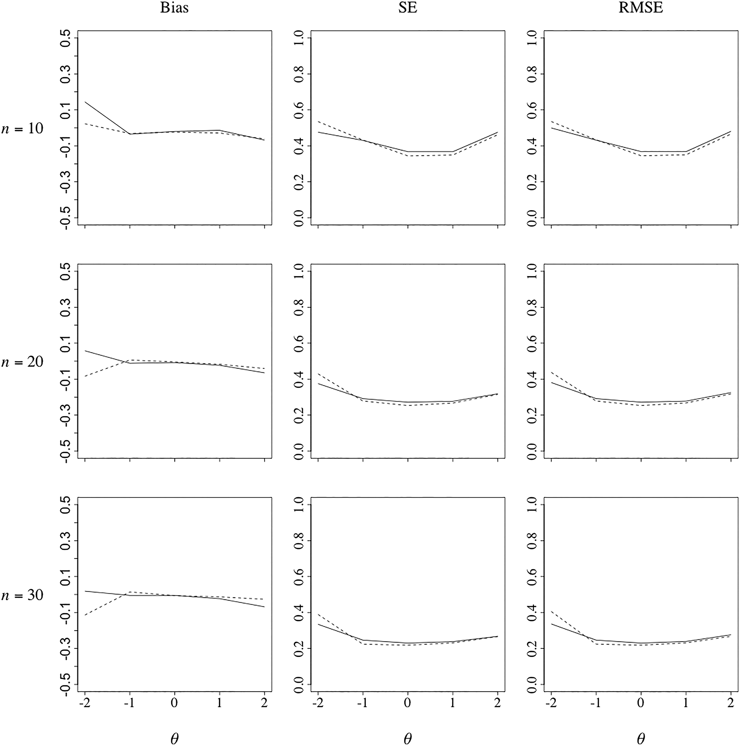
Bias, standard error, and root mean square error of the final ability estimates as a function of θ for adaptive test of n = 10, 20, and 30 items and a calibration sample size of N = 1,000 (solid curves: Bayesian algorithm; dashed curves: maximum information algorithm).

The major lesson the authors learned from this last study was that the reward for the honesty of the Bayesian approach about parameter uncertainty in adaptive testing was not so much direct compensation for the expected increase in the SE of its final ability estimates as a reduction of the bias these estimates might have occurred otherwise. The net effects tended to be positive at the lower end of the scale where estimation error generally tends to be more prominent due to the effects of guessing. We expect these effects to be less prominent under the 2PL model. But adaptive testing does require items that are scorable in real time. Every major adaptive testing program the authors are aware of use multiple-choice items for this reason, a condition under which the 2PL model is unlikely to show satisfactory fit to the response data.

Concluding Remarks

The proposed MCMC algorithm, with its exploiting both of the special structure of the posterior distributions of the item and ability parameters and the sequential nature of adaptive testing, appears to be simple and fast. Running times for a conservative configuration of the algorithm of 0.015 seconds or less per item, as reported above, are low enough for application in real-world adaptive testing.

It is easy to generalize the algorithm to other than the 3PL model used in this article. The change would only involve the substitution of two different expressions, one for the Fisher information in Equation 5 and the other for the probability function $f (u_{i_{k}}; θ, ξ_{i_{k - 1}})$ in the acceptance probability in Equation 14. The mechanics for the draws from the posterior distribution of all model parameters would remain the same. But, of course, extra study would be necessary to confirm whether the current choices of 500 independent posterior draws for the item parameters, 250 burn-in iterations, and 5,000 post-burn-in iterations with thinning by a factor of 10 would still be conservative when moving to a different type of response model. Although the authors have experience with other models and item pools indicating strong robustness of the current choices to such changes, they recommend against blind application of their present results. The best way to proceed is run an additional simulation study using the current choices as starting point to check on their robustness.

	Mean	SD	RMSE
250	.105	.097	.029	.276	.305	.067	.276	.319	.073
500	.018	.090	.025	.247	.243	.063	.247	.258	.068
1,000	.025	.048	.015	.206	.177	.059	.207	.183	.061

Size	k	$θ = - 2$	$θ = - 1$	$θ = 0$	$θ = 1$	$θ = 2$
250	1	61(38)	60(39)	64(46)	76(56)	69(44)
6	60(40)	65(47)	58(38)	64(40)	70(44)
11	69(43)	70(49)	68(46)	67(44)	67(56)
16	66(44)	63(43)	70(42)	67(44)	65(42)
21	71(46)	65(44)	64(44)	71(45)	66(42)
26	70(45)	65(44)	67(46)	69(49)	76(51)
500	1	69(47)	72(50)	70(52)	74(49)	64(45)
6	64(50)	68(52)	68(45)	57(39)	70(47)
11	72(51)	61(39)	68(44)	67(46)	68(44)
16	67(47)	66(48)	65(43)	74(49)	71(49)
21	69(45)	67(52)	68(49)	71(55)	73(48)
26	72(50)	66(43)	74(48)	66(48)	67(44)
1,000	1	61(37)	66(42)	68(39)	79(54)	87(61)
6	73(56)	64(40)	61(46)	72(49)	60(44)
11	68(49)	74(46)	56(39)	67(47)	65(46)
16	66(43)	64(42)	75(51)	74(48)	62(43)
21	70(52)	70(45)	76(48)	63(44)	65(47)
26	76(51)	62(45)	76(53)	69(48)	69(44)

Footnotes

Declaration of Conflicting Interests

The author(s) declared no potential conflicts of interest with respect to the research, authorship, and/or publication of this article.

Funding

The author(s) received no financial support for the research, authorship, and/or publication of this article.

References

Chang

H.-H.

Ying

(2009). Nonlinear sequential design for logistic item response models with applications to computerized adaptive tests. The Annals of Statistics, 37, 1466–1488.

Cheng

Patton

J. M.

Shao

. (2015). α-stratified computerized adaptive testing in the presence of calibration error. Educational and Psychological Measurement, 75, 260–283.

Gelman

Carlin

J. B.

Stern

Dunson

D. B.

Vehtari

Rubin

D. B.

(2014) Bayesian data analysis (3rd ed.). Boca Raton, FL: Chapman & Hall/CRC.

Gelman

Rubin

D. B.

(1992). Inference from iterative simulation using multiple sequences. Statistical Science, 7, 457–511.

Gilks

W. R.

Richardson

Spiegelhalter

D. J.

(1996). Introducing Markov chain Monte Carlo. In Gilks

W. R.

Richardson

Spiegelhalter

D. J.

(Eds.), Markov chain Monte Carlo in practice (pp. 1–19). London, England: Chapman & Hall.

Hambleton

R. K.

Jones

R. W.

(1994). Item parameter estimation errors and their impact on test information functions. Applied Measurement in Education, 7, 171–186.

Hambleton

R. K.

Jones

R. W.

Rogers

H. J.

(1993). Influence of parameter estimation errors in test development. Journal of Educational Measurement, 30, 143–155.

Makransky

Glas

G. A. W.

(2010). An automatic online calibration design in adaptive testing. Journal of Applied Testing Technology, 11. Retrieved from http://www.testpublishers.org/mc/page.do?sitePageId=112031&orgId=atpu.

Owen

R. J.

(1969). A Bayesian approach to tailored testing (Research bulletin 69-92). Princeton, NJ: Educational Testing Service.

10.

Owen

R. J.

(1975). A Bayesian sequential procedure for quantal response in the context of adaptive mental testing. Journal of the American Statistical Association, 70, 351–356.

11.

Patton

Cheng

Yuan

K. -H.

Diao

(2013). The influence of item calibration error on variable-length computerized adaptive testing. Applied Psychological Measurement, 37, 24–40.

12.

Plummer

. (2017). JAGS: Just another Gibbs samples (version 4.3.0) [Computer software]. Retrieved from http://www.mcmc-jags.sourceforce.net

13.

Stocking

M. L.

(1994). Three practical issues for modern adaptive testing item pools (Research report 94-5). Princeton, NJ: Educational Testing Service.

14.

Tsutakawa

R. K.

Johnson

J. C.

(1990). The effect of the uncertainty of item parameter estimation on ability estimates. Psychometrika, 55, 371–390.

15.

Tsutakawa

R. K.

Soltys

M. J.

(1988) Approximation for Bayesian ability estimation. Journal of Educational and Behavioral Statistics, 13, 117–130.

16.

van der Linden

W. J.

(2018). Adaptive testing. In van der Linden

W. J.

(Ed.), Handbook of item response theory. Volume 3: Applications (pp. 197–227). Boca Raton, FL: Chapman & Hall/CRC.

17.

van der Linden

W. J.

Glas

C. A. W.

(2000). Capitalization on item calibration error in adaptive testing. Applied Measurement in Education, 12, 35–53.

18.

van der Linden

W. J.

Glas

C. A. W.

(2001) Cross-validating item parameter estimation in computerize adaptive testing. In Boomsma

van Duijn

M. A. J.

Snijders

T. A. M.

(Eds.), Essays on item response theory (pp. 205–219). New York, NY: Springer.

19.

van der Linden

W. J.

Pashley

P. J.

(2010). Item selection and ability estimation adaptive testing. In van der Linden

W. J.

Glas

C. A. W.

(Eds.), Elements of adaptive testing (pp. 3–30). New York, NY: Springer.

20.

van der Linden

W. J.

Ren

(2015). Optimal Bayesian adaptive design for test-item calibration. Psychometrika, 80, 263–288.

	Mean			SD			RMSE
Sample Size	a_i	b_i	c_i	a_i	b_i	c_i	a_i	b_i	c_i
250	.105	.097	.029	.276	.305	.067	.276	.319	.073
500	.018	.090	.025	.247	.243	.063	.247	.258	.068
1,000	.025	.048	.015	.206	.177	.059	.207	.183	.061